Cosmological observations in scalar-tensor quintessence

Abstract

The framework for considering the astronomical and cosmological observations in the context of scalar-tensor quintessence in which the quintessence field also accounts for a time dependence of the gravitational constant is developed. The constraints arising from nucleosynthesis, the variation of the constant, and the post-Newtonian measurements are taken into account. A simple model of supernovae is presented in order to extract the dependence of their light curves with the gravitational constant; this implies a correction when fitting the luminosity distance. The properties of perturbations as well as CMB anisotropies are also investigated.

I Introduction

The combination of recent astrophysical and cosmological observations (among which are the luminosity distance versus redshift relation up to $z\sim 1$ from type Ia supernovae [1], the cosmic microwave background temperature anisotropies [2] and gravitational lensing [3]) seems to indicate that the universe is accelerating and thus that about $70\%$ of the energy density of the universe is made of a matter with a negative pressure (i.e., having an equation of state $\omega\equiv P/\rho<0$). This raises the natural question of the physical nature of this matter component. Indeed, a solution would be to have a cosmological constant (for which $\omega=-1$) but one will then have to face the well known cosmological constant problem [4], i.e., the fact that the value of this cosmological constant inferred from the cosmological observation is extremely small — about 120 order of magnitude — compared with the energy scales of high energy physics (Planck, grand unified theory, strong and even electroweak scales). Another solution is to argue that there exists a (yet unknown) mechanism which makes the cosmological constant strictly vanish and to find another matter candidate able to explain the cosmological observations. Indeed it assumes that the cosmological constant problem is somehow solved and replaces it by a dark energy problem.

This latter route has gained a lot of enthusiasm in the past years and many candidates have been proposed (for recent reviews on see, e.g., Refs. [5, 6]). Among all these proposals, quintessence [7, 8, 9] seems to be the most promising mechanism. In these models, a scalar field is rolling down a potential decreasing to zero at infinity (often referred to as a runaway potential) hence acting as a fluid with an equation of state varying in the range $-1\leq\omega<1$ if the field is minimally coupled. Runaway potentials such as the exponential potential and inverse power law potentials

$$V(\phi)=\frac{M^{4+\alpha}}{\phi^{\alpha}},$$ (1)

with $\alpha>0$ and $M$ a mass scale, can be found in models where supersymmetry is dynamically broken [10] and in which flat directions are lifted by nonperturbative effects.

As clearly explained in Ref. [11], all the models for this dark energy have to (i) show that they do not contain in a disguise way a cosmological constantlike fine-tuning (the fine-tuning problem), (ii) explain why this kind of matter starts to dominate today (the coincidence problem), (iii) give an equation of state compatible with the observational data (the equation of state problem) and (iv) arise from some high energy physics mechanisms (the model building problem). Quintessence models mainly solved the fine-tuning problem because of the existence of tracking solutions [12] (first studied in Ref. [7, 8]) which are scaling attractor solutions of the field equations and allows the initial conditions for the scalar field to vary by about 150 orders of magnitude. The second tuning (related to the coincidence) concerns the mass scale $M$ that has to be determined by the requirement that about $70\%$ of the energy density of the universe is in the quintessence field. As shown in Ref. [13] for the case of the inverse power law potential, this mass scale is comparable to other scales from high energy physics and the tuning on this mass scale is mild provided the exponent $\alpha$ is not too small ($\alpha$ must be bigger than $4$ so that $M>1\,{\mbox{TeV}}$). The equation of state depends on the shape of the potential and it is hoped that it will be soon determined by, e.g., a weak lensing experiment [14]. For instance, it has been shown that an exponential potential cannot lead to an accelerating universe [7, 8] and that the equation of state for an inverse power law potential mainly depends on the slope $\alpha$. As explained above, the model building is also addressed in the framework of supersymmetry

Quintessence scenarios, however, have some important problems. The requirement of slow roll (mandatory to have a negative pressure) and the fact that the quintessence field dominates today imply that (i) it is very light [15] (roughly of the order $\sim 10^{-33}\,{\mbox{eV}}$ and it should induce violation of the equivalence principle and time variation of the gravitational constant) and that (ii) the vacuum expectation value of the quintessence field today is of order of the Planck mass. This latter problem led Brax and Martin [11, 16] to propose that a supergravity correction had to be taken into account leading to the so-called supergravity (SUGRA) quintessence potential

$$V(\phi)=\frac{M^{4+\alpha}}{\phi^{\alpha}}e^{\frac{1}{2}{\phi^{2}}/{M_{\SS}{\rm Pl}^{2}}},$$ (2)

which shares the same properties as the inverse power law potential at early time but which stabilizes the quintessence field accounting for a better agreement of the equation of state.

Note that the two main features of a quintessence potential is that it must be steep enough for the field to be in a kinetic regime for a large set of initial conditions, hence redshifting faster than radiation and being subdominant at nucleosynthesis, and then to reach a slow roll regime to mimic a cosmological constant. This latter regime will always ultimately take place and the parameters of the potential have to be tuned so that it happens around today. The simplest waya to implement this idea are to use inverse power law potentials and exponential potentials which are one parameter potentials. Another solution (but involving more parameters) is to consider potentials with a local minimum as was first proposed by Wetterich [8].

An underlying motivation to replace the cosmological constant by a time dependent scalar field probably lies in string models in which any dimensionful parameter is expressed in terms of the fundamental string mass scale and the vacuum expectation value of a scalar field. For instance, string theory has revived the consideration of gravitational-strength scalar fields [17] such as Kaluza-Klein moduli or the dilaton appearing in the low energy limit of the gravitational sector leading to scalar-tensor theories of gravity. As explained above, the quintessence field is expected to be very light and this points toward scalar-tensor theories of gravity in which a light (or massless) scalar field can be present in the gravitational sector without being phenomenologically disastrous. These arguments lead to consider quintessence models in the framework of scalar-tensor gravity. Indeed, the dilaton and the quintessence field can be two different scalar fields (as considered, e.g., in Ref. [18] in the particular case of Brans-Dicke theory) or the same scalar field. The latter subclass involving a single scalar field (the quintessence field is also the dilaton) dictating the time variation of both the gravitational constant and the cosmological constant is attractive; it involves less free functions and has been focused on much in recent years. The study of these quintessence models, referred to as nonminimal quintessence [19], coupled quintessence [20], extended quintessence [21] or generalized quintessence [22] was mainly motivated by the fact that tracking solutions have been shown to exist for nonminimally coupled scalar fields [19, 26].

Scalar-tensor theories are the most natural extensions of general relativity, in particular they contain local Lorentz invariance, constancy of nongravitational constants and respect the weak equivalence principle. The most general action for these theories [23] for the matter and gravity is given, in the Jordan frame, by

$$S=\int\left[-F(R,\phi)+\frac{1}{2}\frac{\omega(\phi)}{\phi}\partial_{\mu}\phi\partial^{\mu}\phi-V(\phi)+{\cal L}_{\SS}{\rm mat}\right]\sqrt{-g}{\rm d}^{4}x,$$ (3)

where ${\cal L}_{\SS}{\rm mat}$ is the Lagrangian of ordinary matter (such as radiation and pressureless matter), $g$ is the determinant of the metric $g_{\mu\nu}$, $R$ the Ricci scalar, and $V$ is a potential to be discussed below. The action (3) depends a priori on three arbitrary functions $F$, $\omega$, and $V$. If $F(R,\phi)$ is not a trivial function of $R$ then one has an additional (massive) scalar degree of freedom [24] so that the requirement that there is only one scalar partner to the graviton implies

$$F(R,\phi)=\frac{1}{2\kappa}F(\phi)R,$$ (4)

where $\kappa\equiv 8\pi G\equiv M_{\SS}{\rm Pl}^{2}$, $G$ being the bare Newton constant. $F(\phi)$ is a dimensionless function which needs to be positive to ensure that the graviton carries positive energy [25]. Now, by a redefinition of $\phi$ we can always choose either $F(\phi)$ or $\omega(\phi)/\phi$ to be unity so that we are left with only two independent functions of the scalar field one being the potential $V$. Choosing $\omega(\phi)/\phi=1$, the effective (time dependent) constant is related to $G$ by

$$G_{\SS}{\rm eff}(\phi)\equiv\frac{G}{F(\phi)}.$$ (5)

As was explained above, authors first considered models with a nonminimally coupled scalar field [19, 26, 27, 28], i.e., in which the function $F$ is decomposed as

$$F(\phi)=1+2\xi\kappa f(\phi).$$ (6)

Indeed, as long as we have not fixed the choice of the function $f$, such a decomposition is completely general and always possible. If the normalization of $f$ is chosen in a way that $f(M_{\SS}{\rm Pl})\sim{\cal O}(M_{\SS}{\rm Pl}^{2})$ today then $\xi$ gives an order of magnitude of the deviation with respect to general relativity today.

Due to the time variation of the gravitational constant, the strength of the coupling $\xi$ can be constrained once the function $f(\phi)$ has be chosen. Chiba [29] gave the constraints arising from the post-Newtonian (PN) parameters and the time variation of $G$ for $f=\phi^{2}/2$. In that case the deviation of the scalar-tensor theory from general relativity was fixed but, as pointed out by Bartolo and Pietroni [30] in scalar-tensor quintessence models a “double attractor mechanism” can happen, namely, of the scalar-tensor theory towards general relativity (through the Damour-Nordtvedt mechanism [31]) and of the quintessence field toward its tracking solution hence allowing for large deviation from general relativity in the early universe. Note that in these models the dilaton is not completely stabilized and is slow rolling in its runaway potential.

Many works have then studied the cosmological implications of these models, starting from the study of the perturbations in Brans-Dicke theory [32] and for a nonminimally coupled scalar field [33, 34] the computation of cosmic microwave background (CMB) anisotropies [21, 35], the properties of the nucleosynthesis [30, 36]. But among all, one of the very interesting results concerns the possibility to rule out some of these models [22]: it was shown that because of the positivity of the energy of the graviton, one can mimic a model in which the gravity is described by general relativity with a cosmological constant by a scalar-tensor theory with $V=0$ (or when certain relation between $V$ and $F$ are set) only in a certain range of redshift, hence offering a powerful test on a large class of scalar-tensor models.

In this article, we try to extract the observational constraints on these quintessence models in scalar-tensor gravity. We first recall in Sec. II the background properties: we study the constraints arising from the bounds on the post-Newtonian parameters, the time variation of the gravitational constant, of nucleosynthesis and of the positivity of the energy of the graviton. We then turn to the information that can be extracted for the type Ia supernovae (Sec. II B). This lead us to describe a simple model of SN Ia in order to extract the dependence of the light curve with the gravitational constant and give us a modified magnitude vs redshift relation that has to be used when extracting the luminosity distance vs redshift relation. We finish by a computation of the angular diameter distance vs redshift relation (Sec. II C). We then turn to the property of the perturbations and generalize the attractor property (Sec. III) found in Ref. [37] to the scalar-tensor quintessence and then discuss the CMB angular spectrum (Sec. IV). All the technical details are gathered in the appendices and we apply these results all along the article to two examples, one being a nonminimally coupled scalar field and the second a scalar-tensor theory with conformal coupling.

II Background properties

We consider a Friedmann-Lemaître universe with the line element

$${\rm d}s^{2}={\rm d}t^{2}-a^{2}(t)\gamma_{ij}{\rm d}x^{i}{\rm d}x^{j}\equiv g_{\mu\nu}{\rm d}x^{\mu}{\rm d}x^{\nu},$$ (7)

where $a$ is the scale factor, $t$ the cosmic time and $\gamma_{ij}$ the metric on constant time hypersurfaces. Greek indices run from 0 to 3 and Latin indices from 1 to 3. As detailed in Appendix B, the Friedmann equation in presence of a nonminimally coupled scalar field takes the form

$${\cal H}^{2}+K=\frac{\kappa_{\SS}{\rm eff}}{3}a^{2}\left(\rho_{\SS}{\rm mat}+\rho_{\SS}{\rm MC}+\rho_{\SS}{\rm\xi}\right),$$ (8)

where we have introduced the conformal Hubble parameter ${\cal H}\equiv\dot{a}/a$, and where an overdot denotes a derivative with respect to the conformal time (${\rm d}t=a{\rm d}\eta$), and $K$ is the curvature index. On the right-hand side, $\rho_{\SS}{\rm mat}$ designs the matter energy density, and $\rho_{\SS}{\rm MC}$ and $\rho_{\SS}{\rm\xi}$, the energy densities of the scalar field and respectively defined respectively in Eqs. (B8) and (B10). The quantity $\kappa_{\SS}{\rm eff}\equiv\kappa/F(\phi)$ acts as an effective Newton constant and depends also on $\phi$ (and hence, varies with time). We define the density parameter of any component $f$ by

$$\Omega_{\SS}{f}\equiv\frac{\kappa_{\SS}{\rm eff}a^{2}\rho_{\SS}{f}}{3{\cal H}^{2}},$$ (9)

where one has to use $\kappa_{\SS}{\rm eff}$ and not $\kappa$ since we have only access to a measure of the effective Newton constant and not of its bare value.

A How is $F(\phi)$ constrained?

In this section, we review the different constraints on $F(\phi)$ arising from the requirement of the positivity of the energy of the graviton, the bounds on the post-Newtonian parameters and of the time variation of the gravitational constant and from nucleosynthesis.

1. Positivity of the energy of the graviton: Diagonalizing the action (3) by the conformal transformation [25]

   $$\widetilde{g}_{\mu\nu}\equiv F(\phi)g_{\mu\nu},\quad\left(\frac{{\rm d}\widetilde{\phi}}{{\rm d}\phi}\right)^{2}\equiv\frac{3}{4}\left(\frac{{\rm d}\ln F(\phi)}{{\rm d}\phi}\right)^{2}+\frac{1}{2F(\phi)},\quad A(\widetilde{\phi})\equiv F^{-1/2}(\phi),\quad 2U(\widetilde{\phi})\equiv\frac{V(\phi)}{F^{2}(\phi)},$$ (10)

   one can show that the graviton is the perturbation of $\widetilde{g}_{\mu\nu}$ and its scalar partner $\widetilde{\phi}$ evolving in the potential $U(\widetilde{\phi})$. It can be shown that a scalar-tensor theory in fact well defined only if the transformation (10) is possible [22, 25]. This is the case if $F(\phi)$ is positive. When integrating our equations this constraint has to be checked. In practice, since one has $\kappa_{\SS}{\rm eff}\propto F^{-1}\propto{\cal H}^{2}+K$, this constraint is always satisfied when the universe is spatially flat.

2. Post-Newtonian constraints: With the form (3), the standard post-Newtonian parameters are given by [23, 25]

   $$\gamma_{\SS}{\rm PN}-1 = \frac{\left(F^{\prime}_{0}\right)^{2}}{M_{\SS}{\rm Pl}^{2}F_{0}+2\left(F^{\prime}_{0}\right)^{2}}=-2\frac{\alpha_{0}^{2}}{1+\alpha_{0}^{2}},$$ (11)

   $$\beta_{\SS}{\rm PN}-1 = \frac{1}{4}\frac{F_{0}F^{\prime}_{0}}{2M_{\SS}{\rm Pl}^{2}F_{0}+3\left(F^{\prime}_{0}\right)^{2}}\frac{{\rm d}\gamma_{\SS}{\rm PN}}{{\rm d}\phi}=\frac{1}{2}\frac{\alpha_{0}^{2}}{(1+\alpha_{0}^{2})^{2}}\frac{{\rm d}\alpha_{0}}{{\rm d}\widetilde{\phi}},$$ (12)

   where a dash denotes a derivative with respect to the field $\phi$ and where a subscript $0$ means that the function is evaluated today. The function $\alpha$ is defined by

   $$\alpha(\widetilde{\phi})\equiv\frac{{\rm d}\ln A}{{\rm d}\widetilde{\phi}}.$$ (13)

   Current constraints (see, e.g., Ref. [38] for a recent review of the measurements) give

   $$\left|\gamma_{\SS}{\rm PN}-1\right|\leq 2\times 10^{-3},\quad\left|\beta_{\SS}{\rm PN}-1\right|\leq 6\times 10^{-4}.$$ (14)

   This implies that

   $$\alpha_{0}^{2}\sim\frac{1}{M_{\SS}{\rm Pl}^{2}F_{0}}\left(F^{\prime}_{0}\right)^{2}<10^{-3},$$ (15)

   and, as explained in Ref. [22], the second bound cannot be used to constraint ${\rm d}\alpha_{0}/{\rm d}\phi$.

3. Time variation of $G$: The effective constant $G_{\SS}{\rm eff}$ deduced from Eq. (5) is not the gravitational constant that would be measured in a Cavendish-Michel-type experiment, i.e., it is not the effective Newton constant. This constant $G_{{\rm N}_{\SS}{\rm eff}}$, entering in the force between two masses, is given by

   $$G_{{\rm N}_{\SS}{\rm eff}}=\frac{G}{F_{0}}\frac{2M_{\SS}{\rm Pl}^{2}F_{0}+4\left(F^{\prime}_{0}\right)^{2}}{2M_{\SS}{\rm Pl}^{2}F_{0}+3\left(F^{\prime}_{0}\right)_{0}^{2}}=GA_{0}^{2}(1+\alpha_{0}^{2}),$$ (16)

   in which one has two contributions, namely the exchange of a graviton and of a scalar [25]. Current constraints [39] on the variation of the Newton constant imply

   $$\left|\frac{\dot{G}_{{\rm N}_{\SS}{\rm eff}}}{G_{{\rm N}_{\SS}{\rm eff}}}\right|\leq 6\times 10^{-12}\,{\mbox{yr}^{-1}}.$$ (17)

4. Nucleosynthesis: Nucleosynthesis bounds have two origins. Roughly speaking, we have to require that (i) the matter contents dominating the Friedmann equation behaves as radiation at nucleosynthesis and that (ii) the effective number of degrees of freedom of the relativistic particles, $g_{*}$ say, does not vary from more than $20\%$ than its expected value $g_{*}=10.75$ at this epoch.

   In the case of quintessence with an exponential potential, these bounds were used to show that the quintessence field can not close the universe [40]. For general inverse power law and SUGRA potentials, the first constraint was shown [13] to imply bounds on the initial condition of the scalar field at the end of inflation. Here, we want to estimate the bounds arising from the second requirement and we assume that the contribution of the scalar field is subdominant with respect to the radiation. The energy density of the radiation is given by

   $$\rho_{\SS}{\rm rad}=\frac{\pi^{2}}{30}g_{*}T^{4},$$ (18)

   where $T$ is the temperature. Assuming that $\rho_{\SS}{\rm Q}\ll\rho_{\SS}{\rm rad}$ [$\rho_{\SS}{\rm Q}$ being defined by Eq. (B18)], the Friedmann equation (8) leads to

   $${\cal H}^{2}=\kappa_{0}a^{2}\frac{\pi^{2}}{90}g_{*}\left(1+\frac{\delta g_{*}}{g_{*}}\right)T^{4},$$ (19)

   with

   $$\frac{\delta g_{*}}{g_{*}}\equiv\left(\frac{\kappa_{\SS}{\rm eff}}{\kappa_{0}}-1\right)=\frac{F(\phi_{0})-F(\phi_{\SS}{\rm nuc})}{F(\phi_{\SS}{\rm nuc})},$$ (20)

   where $\phi_{\SS}{\rm nuc}$ is the value of $\phi$ at the time of nucleosynthesis. Nucleosynthesis therefore imposes that

   $$\left|\frac{\delta g_{*}}{g_{*}}\right|\leq 0.2\Longleftrightarrow 0.8\leq\left|\frac{F(\phi_{0})}{F(\phi_{\SS}{\rm nuc})}\right|=\left|\frac{A^{2}(\phi_{\SS}{\rm nuc})}{A^{2}(\phi_{0})}\right|\leq 1.2.$$ (21)

   This constraint, in the framework of quintessence, was first derived by Bartolo and Pietroni [30]. It was also shown [36] numerically that in some nonminimally coupled quintessence models the Helium abundance can be reduced extending the upper limit on the number of neutrino to 5. Let us also emphasize that very large values of $|{F(\phi_{0})}/{F(\phi_{\SS}{\rm nuc})}|$ were shown [41] to be consistent with the observed abundances of light elements if ${\rm d}^{2}A/{\rm d}\widetilde{\phi}^{2}$ is large enough. Hence, the naive limit (21) can be much more stringent than a detailed (numerical) study may show.

1 Nonminimally coupled scalar field

As a first example, we consider the case of the nonminimally scalar field introduced in Ref. [19] for which

$$F(\phi)=1+2\xi\kappa f(\phi),$$ (22)

and we choose the function $f$ to be

$$f(\phi)=\frac{1}{2}\phi^{2}.$$ (23)

In Fig. 1, we depict the typical evolution of the equation of state parameter $\omega_{\SS}{\rm Q}\equiv P_{\SS}{\rm Q}/\rho_{\SS}{\rm Q}$ of the quintessence field and the time variation of the Newton constant in the minimally coupled and nonminimally coupled cases. As explained in the appendices, the equation of state parameter of the quintessence field has two distinct contributions: $\omega_{\SS}{\rm MC}$ that appears in the minimally coupled case, and an extra contribution $\omega_{\SS}{\rm\xi}$ that appears only in the non minimally coupled case. $\omega_{\SS}{\rm Q}$, $\omega_{\SS}{\rm MC}$, and $\omega_{\SS}{\rm\xi}$ are related by

$$\omega_{\SS}{\rm Q}=\frac{\rho_{\SS}{\rm MC}}{\rho_{\SS}{\rm MC}+\rho_{\SS}{\rm\xi}}\omega_{\SS}{\rm MC}+\frac{\rho_{\SS}{\rm\xi}}{\rho_{\SS}{\rm MC}+\rho_{\SS}{\rm\xi}}\omega_{\SS}{\rm\xi}.$$ (24)

It can be trivially checked that when the tracking solution is reached,

$$\omega_{\SS}{\rm\xi}=-\frac{1}{3}.$$ (25)

Now, a subtlety arises from the fact that depending on the sign of $\xi$, the quantity $\rho_{\SS}{\rm\xi}$ can be negative. In this case, $\omega_{\SS}{\rm Q}$ does not lie between $\omega_{\SS}{\rm\xi}$ and $\omega_{\SS}{\rm MC}$. With our conventions, $\rho_{\SS}{\rm\xi}$ and $\xi$ are of opposite sign. In both cases one finds, however, that the field reaches Planck values as it starts to dominate, i.e., today. Given the form of the coupling function (23), this means that all the departure from general relativity are mostly felt today. This also implies that these departures are stronger in the case of an inverse power-law than in the case of a SUGRA potential, mainly because in the latter case the potential is less steep (due to the exponential term) so that the scalar field is more stabilized and rolls down slower, implying a smaller time variation of the coupling function $F$. Another interesting feature lies in the fact that $\omega_{\SS}{\rm Q}-\left.\omega_{\SS}{\rm Q}\right|_{\xi=0}$ changes sign around $z\simeq 1$.

In Fig. 2, we sum up all the preceding constraints in the plane $(\Omega_{\SS}{\rm Q}^{0},\xi)$ both for the inverse power law (1) and SUGRA potentials (2). Since $\phi\sim M_{\SS}{\rm Pl}$ today, $F(\phi_{0})-1\propto\xi$ and $\xi$ is then a direct measurement of the deviation from general relativity today from which it follows that $\xi$ must be very small today (as first pointed out in Ref. [29]). The constraints are stronger for inverse power law potentials. This is easily understood if one notices that for small $\xi$, the equation of state parameter $\omega$ is higher in the SUGRA case. This translates into a stronger time dependence of the quintessence field, which in turn puts more stringent constraints on the coupling between the scalar field and the metric. This remark therefore extends the bounds obtained in Ref. [29]. In both cases, the most stringent constraint arises from the constraint on the post-Newtonian parameter $\gamma_{\SS}{\rm PN}$ and all these constraints become stronger for high $\Omega_{\SS}{\rm Q}$. Another interesting point would be to study how these bounds depend on $\alpha$. For the Ratra-Peebles potential, this was already addressed in Chiba’s work: the bound on $\xi$ varies as $\alpha^{-1}$, which can be checked numerically. For the SUGRA potential, the answer is even simpler: the dynamics of the quintessence field varies very weakly with $\alpha$ [11]. Therefore, the bound on $\xi$ are not significantly dependent on $\alpha$.

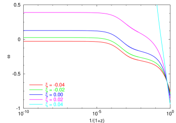
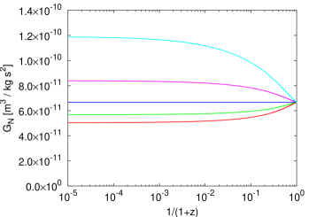
FIG. 1.: Evolution of the quintessence equation of state parameter $\omega_{\SS}{\rm Q}$ as a function of the redshift $z$ for $\Omega_{\SS}{\rm Q}=0.7$ and various values of the coupling parameter $\xi$ (left). For negative $\xi$, $-\frac{1}{3}<\omega_{\SS}{\rm Q}<\omega_{\rm B}$ in the tracking regime, whereas this condition does not hold for positive $\xi$. This is due to the fact that $\rho_{\SS}{\rm\xi}$ is negative when $\xi$ is positive. For all the models presented here, $\omega_{\SS}{\rm Q}-\left.\omega_{\SS}{\rm Q}\right|_{\xi=0}$ changes sign around $z\simeq 1$. Evolution of the gravitational constant as a function of the redshift $z$ for various values of the coupling parameter $\xi$ (right). The color codes are identical in the two plots.

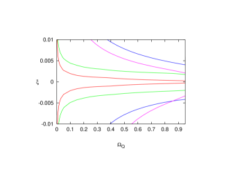
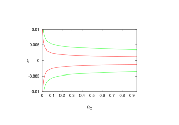
FIG. 2.: Summary of the constraints on the parameters ($\xi$, $\Omega_{\SS}{\rm Q}^{0}$) for an inverse power law potential with $\alpha=11$ (left) and for a SUGRA potential with $\alpha=11$ (right). The allowed region lies between the lines of same color. The red lines represent the constraint arising from the $\gamma_{\SS}{\rm PN}$ post Newtonian parameter [see Eq. 11], the green line is from $\beta_{\SS}{\rm PN}$, the blue line from the time-variation of $G_{{\rm N}_{\SS}{\rm eff}}$, and the purple line from nucleosynthesis. In both cases, the most stringent constraint comes from $\gamma_{\SS}{\rm PN}$ and are stronger for high $\Omega_{\SS}{\rm Q}$.

2 Exponential coupling

As a second example, we shall consider the class of scalar-tensor models in which the coupling function $A$ is given by

$$A_{\SS}{\rm EX}(\widetilde{\phi})=Be^{-\beta\widetilde{\phi}},$$ (26)

with either the inverse power law or SUGRA potentials as defined in Eqs. (1) and (2).

To compare with, the standard Damour-Nordtvedt mechanism of attraction of scalar-tensor theories towards general relativity, one requires the coupling constant $\alpha$ to drive the field towards its minimum where $\phi=0$. In the case of quintessence, the field evolves toward infinity at late time and we would need to consider a coupling function $\alpha$ such as

$$\alpha_{\SS}{\rm DN}(\widetilde{\phi})=-Be^{-\beta\widetilde{\phi}},$$ (27)

that tends to zero at infinity in order to converge toward general relativity. The function $A$ is easily obtained by integrating Eqs. (13), (27) to give

$$\ln\frac{A_{\SS}{\rm DN}}{A_{\SS{\rm DN},i}}=-\frac{1}{\beta}\left[\alpha_{\SS}{\rm DN}(\widetilde{\phi})-\alpha_{\SS}{\rm DN}(\widetilde{\phi}_{i})\right],$$ (28)

where the subscript $i$ refers to some initial time. On the contrary, the class of models (26) does not exhibit the double attractor mechanism [30] because $\alpha$ and hence, the PN parameter $\gamma_{\SS}{\rm PN}$ are constant: one has $\alpha_{\SS}{\rm EX}=-\beta$, $\gamma_{\SS}{\rm PN}^{\SS}{\rm EX}\sim 1-2\beta^{2}$, and $\beta^{\SS}{\rm EX}_{\SS}{\rm PN}=0$. therefore, as long as $\beta$ is sufficiently small (we shall take $\beta=0.025$ in the following), this model can be compatible with the Solar system constraints. Note that in this model, the constancy of $\alpha_{\SS}{\rm EX}$ requires that the coupling function $F$ is a polynomial of degree $2$, exactly as in the first example. The class of models (27) can indeed be easily studied along similar lines.

In Fig. 3, we show the evolution of the equation of state parameter $\omega$ and the Newton constant with time. In Fig. 4, we sum up all the constraints detailed above in the plane $(\Omega_{\SS}{\rm Q}^{0},B)$. As already noted, the constraint on the PN parameter $\beta_{\SS}{\rm PN}$ is trivially verified, and the constraint on $\gamma_{\SS}{\rm PN}$ is also satisfied as long as the parameter $\beta$ in Eq. (26) is small. Therefore, only the two other constraints play a role, in contrast with the former case.

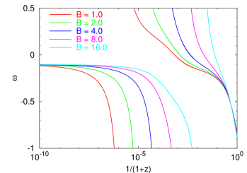
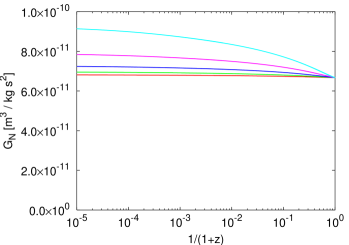
FIG. 3.: Evolution of the quintessence equation of state parameter $\omega_{\SS}{\rm Q}$ (left) and of the Newton “constant” $G_{{\rm N}_{\SS}{\rm eff}}$ (right) as a function of the redshift $z$ for $\Omega_{\SS}{\rm Q}^{0}=0.7$, $\beta=0.0025$, and various values of the coupling parameter $B$.

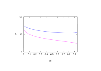
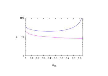
FIG. 4.: Summary of the constraints on the parameters ($B,\Omega_{\SS}{\rm Q}^{0}$) in the case of a Ratra-Peebles (left) and SUGRA (right) potential with $\alpha=11$. The color codes are the same as for Fig. 3.

B Supernovae data

The use of type Ia supernovae to constraint the cosmological parameters (and hence the claim that our universe is accelerating) mostly lies in the fact that we believe that they are standard candles so that we can reconstruct the luminosity distance vs redshift relation and compare it with its theoretical value. In a scalar-tensor theory, we have to address both questions, i.e., the determination of the luminosity distance vs redshift relation (Sec. II B 1) and the property of standard candle since two supernovae of different redshift are feeling a different gravitational coupling constant and may not be standard candles anymore (Sec. II B 2).

1 Luminosity distance in scalar-tensor theories

To derive the luminosity distance (${\rm d}_{\SS}{\rm L}$) vs redshift ($z$) relation needed to interpret the supernovae data, we rewrite Eq. (8) as

$$\left(\frac{{\cal H}}{{\cal H}_{0}}\right)^{2}\equiv E^{2}(x)=\frac{\kappa_{\SS}{\rm eff}}{\kappa_{\SS}{\rm eff}^{0}}\left[\Omega_{\SS}{\rm mat}^{0}x^{-1}+\Omega_{\SS}{\rm rad}^{0}x^{-2}+\Omega_{\SS}{\rm Q}^{0}\frac{\rho_{\SS}{\rm Q}(x)}{\rho_{\SS}{\rm Q}(1)}x^{2}\right]+\Omega_{\SS}{K}^{0},$$ (29)

where $x\equiv 1/(1+z)$, and $\Omega_{\SS}{K}^{0}\equiv-K/{\cal H}_{0}^{2}$. The metric of the constant time hypersurfaces is decomposed as

$$\gamma_{ij}{\rm d}x^{i}{\rm d}x^{j}={\rm d}\chi^{2}+\mbox{s}_{\SS{K}}^{2}(\chi){\rm d}^{2}\omega,$$ (30)

where ${\rm d}^{2}\omega$ is the infinitesimal solid angle and $\mbox{s}_{\SS{K}}(\chi)\equiv[\sin(\sqrt{K}\chi)/\sqrt{K},\chi,\sinh(\chi\sqrt{-K})/\sqrt{-K}]$ for $K$, respectively, positive, zero or negative. With these notations, the luminosity distance is given by [42]

$${\rm d}_{\SS}{\rm L}[z;\Omega_{0},\Omega_{\SS}{\rm Q}^{0},\xi]=(1+z)\frac{c}{H_{0}}\mbox{s}_{-\Omega_{\SS}{K}^{0}}\left[\int_{0}^{z}\frac{{\rm d}z^{\prime}}{(1+z^{\prime})E(z^{\prime})}\right].$$ (31)

2 SN Ia in scalar-tensor theories

The standard lore is to compare this result with type Ia supernovae data to extract the cosmological parameters assuming that they are standard candles in the sense that their light curve does not depend on the supernovae and in particular of $z$. A time varying effective gravitational constant can affect this picture at least in two ways [43] by changing

1. the thermonuclear energy release, since the luminosity at the maximum of the light curve is proportional to the mass of nickel synthetized,

2. the time scale of the supernova explosion and hence the width of its light curve.

As we pointed out in the Introduction, it was shown in Ref. [22] that the relation (29) for a flat Cold Dark Matter model with a cosmological constant ($\Lambda$CDM) in the framework of general relativity can be mimicked by a scalar-tensor theory with $V=\Lambda=0$ up to a given redshift. But, this study did not include the fact that in scalar-tensor theories one, as will be shown here, can not directly use the luminosity distance vs redshift relation inferred in the framework of general relativity. Hence, when comparing any scalar-tensor theory to supernovae type Ia (SN Ia) data, one needs a modified magnitude vs redshift relation taking into account the effects listed above. The goal of this section is not to explain the recent SN Ia data by replacing the cosmological constant by a scalar-tensor theory but rather to know how to deal with these data in such a framework and to evaluate the effect of the coupling on the precision of the determination of the cosmological parameters.

To discuss these issues, we recall a simple “one zone” toy model [44, 45] of an expanding sphere of uniform temperature $T$ and density and of radius and mass $R_{\SS}{\rm env}$ and $M_{\SS}{\rm env}$ for the supernovae light curve which encapsulates the main features of dependence in the gravitational constant $G$, even if this model is nothing but a toy model. The observed light curve is obtained from the nonadiabatic evolution of the thermal energy $E_{\SS}{\rm th}=4\pi aT^{4}R_{\SS}{\rm env}^{3}/3$ of the radiation dominated envelope

$$\dot{E}_{\SS}{\rm th}+4\pi PR^{2}_{\SS}{\rm env}\dot{R}_{\SS}{\rm env}=-L+L_{*},$$ (32)

where $L\simeq E_{\SS}{\rm th}/\tau_{\SS}{\rm diff}$ is the bolometric luminosity. $L_{*}=L_{*\,0}\exp[-t/\tau_{*}]$ is the radioactive energy input (from ${}_{56}\mathrm{{\rm Ni}}\rightarrow_{56}\mathrm{{\rm Co}}\rightarrow_{56}\mathrm{{\rm Fe}}$, where $\tau_{*}$ represents the corresponding nuclear process half life time). $P=aT^{4}/3$ is the radiation pressure and the thermal energy $E_{\SS}{\rm th}$ and the photon diffusion time scale $\tau_{\SS}{\rm diff}$ is given by

$$\tau_{\SS}{\rm diff}=3\frac{R_{\SS}{\rm env}^{2}}{\lambda_{\gamma}}\simeq 9\frac{\kappa_{\SS}{\rm Th}M_{\SS}{\rm env}}{4\pi R_{\SS}{\rm env}},$$ (33)

where $\kappa_{\SS}{\rm Th}$ is the Thomson opacity and $\lambda_{\gamma}$ the photons free mean path. Since the temperature scales as $1/R_{\SS}{\rm env}$, it follows that

$$E_{\SS}{\rm th}=\frac{M_{0}}{2}\frac{R_{0}}{R_{\SS}{\rm env}},$$ (34)

where $R_{0}$ and $M_{0}$ are respectively the radius of and the mass of the progenitor. Equation (32) yields the equation for the luminosity $L$

$$\frac{R_{0}}{R_{\SS}{\rm env}}\dot{L}=(-L+L_{*})\frac{1}{\tau_{\SS}{\rm diff}^{0}},$$ (35)

where $\tau_{\SS}{\rm diff}^{0}$ is the initial diffusion time scale when $R_{\SS}{\rm env}=R_{0}$. If the envelope expands at a constant velocity $v_{\SS}{\rm exp}\equiv\dot{R}_{\SS}{\rm env}$, an analytic solution to Eq. (35) was found by Arnett [44] as

$$L=L_{\SS}{\rm P}e^{-u(x)}+L_{*}^{0}\Omega(x,y,w),$$ (36)

where, from Eqs. (33) and (34), $L_{\SS}{\rm P}\simeq E_{\SS}{\rm th}/\tau_{\SS}{\rm diff}\simeq 2\pi R_{0}/9\kappa_{\SS}{\rm Th}$ is the luminosity at the maximum of the light curve, $u(x)\equiv wx+x^{2}$, $x\equiv t/\tau$, $y\equiv\tau/2\tau_{*}$, $\omega\equiv\tau/\tau_{\SS}{\rm diff}^{0}$, and $\tau$ is the characteristic time of the SN given by

$$\tau^{2}=2\frac{R_{0}}{v_{\SS}{\rm exp}}\tau_{\SS}{\rm diff}^{0},$$ (37)

and the function $\Omega$ takes the form

$$\Omega(x,y,w)\equiv e^{-u(x)}\int_{0}^{x}(w+2z)e^{-2zy+u(z)}{\rm d}z.$$ (38)

The expansion velocity can be obtained via the conservation of energy as

$$v_{\SS}{\rm exp}^{2}=2\frac{M_{\SS}{{\rm Ni}}}{M_{0}}.$$ (39)

In order the model to be consistent, we are therefore obliged to assume that $M_{\SS}{{\rm Ni}}\leq\frac{1}{2}M_{0}$. From the above equation, it follows that $\tau$ behaves as

$$\tau^{2}\simeq\frac{9\kappa_{\SS}{\rm Th}}{2\pi\sqrt{2}}\left(\frac{M_{0}^{3}}{M_{\SS}{{\rm Ni}}}\right)^{1/2}.$$ (40)

Assuming that the progenitor has the Chandrasekar mass $M_{\SS}{\rm Ch}$, $R_{0}$ is the Chandrasekar radius, and assuming that the mass of nickel scales as $M_{0}$, we deduce that

$$L_{\SS}{\rm max}=L_{\SS}{\rm max}^{\SS}{\rm GR}\left(\frac{G_{\SS}{\rm eff}}{G}\right)^{-3/2},\quad\tau=\tau^{\SS}{\rm GR}\left(\frac{G_{\SS}{\rm eff}}{G}\right)^{-3/4},$$ (41)

since the total energy release is proportional to mass of nickel formed which is assumed to scale as the progenitor mass and thus as $G^{-3/2}$.

Such a toy model can, at that stage, describe both SN I and SN II. But, for SNIa, the progenitor is a white dwarf and it follows that $R_{0}\sim 5\times 10^{3}\,{\mbox{km}}$. Then, since

$$\tau_{\SS}{\rm diff}^{0}\simeq 10^{8}\frac{M_{\SS}{\rm env}}{M_{\odot}}\left(\frac{R_{0}}{5\times 10^{3}\,{\mbox{km}}}\right)^{-1}$$ (42)

and

$$\tau\simeq 71\frac{M_{\SS}{\rm env}}{M_{\odot}}^{1/2}\left(\frac{v_{\SS}{\rm exp}}{10^{4}\,{\mbox{km}}\,{\mbox{s}^{-1}}}\right)^{-1/2},$$ (43)

we can conclude that $L_{\SS}{\rm P}\simeq 0$ and that $\omega\sim 10^{-7}$. We then choose the typical [45] value of the parameters for SN Ia to be

$$L_{\SS}{\rm P}=0,\quad w=0.$$ (44)

It follows that the luminosity curve is well approximated by $L=L_{*}^{0}\Omega(x,y,0)$ which can be integrated analytically to give

$$L=L_{*}^{0}\left(e^{-2xy}-e^{x^{2}}+i\sqrt{\pi}ye^{-(x^{2}+y^{2})}\left[\hbox{Erf}(ix-iy)+\hbox{Erf}(iy)\right]\right),$$ (45)

where Erf is the error function and where the nuclear rate are given by

$$\mbox{cobalt: }L_{*}=1.5\times 10^{43}M_{\SS}{{\rm Ni}}\,{\mbox{erg}}\,{\mbox{s}^{-1}} ,\quad \tau_{*}=111\,{\mbox{days}},$$ (46)

$$\mbox{nickel: }L_{*}=8\times 10^{43}M_{\SS}{{\rm Ni}}\,{\mbox{erg}}\,{\mbox{s}^{-1}} ,\quad \tau_{*}=10.1\,{\mbox{days}}.$$ (47)

In Fig. 5, we depict a standard light curve obtained with this one zone model and the light curves when $G$ is increased respectively by $10\%$ and $20\%$. This light curves are compared to the ones obtained by a variation of the nickel mass synthetised. The decaying branch is mainly sensitive to the mass of nickel so that an increase of the gravitational constant implies that the light curve has a lower maximum and then tends asymptotically towards the light curve of a supernovae with lower nickel mass. As a conclusion, if $G_{\SS}{\rm eff}$ is $10\%$ larger than $G$ all other parameters being unchanged, then the luminosity at maximum will be slower by about $15\%$ and the time scale $\tau$ will be smaller by $7.5\%$ and the light curve will be narrower. As was realized, supernovae are not exactly standard candles but, thanks to the correlation between the time scale of the light curve and the peak luminosity (larger curves are brighter while narrower are fainter), the dispersion of $0.15$–$0.2\,{\mbox{mag}}$ can be corrected by the use of a stretch factor [1].

A variation of $G$ affects both the amplitude of the peak and the time scale and, for instance, makes it narrower and fainter if $G$ grows in the past. Again, they can be calibrated to extract the luminosity distance since, once the model is specified, the dependence of the correction due to the variation of $G$ is known. The magnitude vs redshift relation then takes the form

$$m(z)={\cal M}_{0}+5\log{\rm d}_{\SS}{\rm L}[z;\Omega_{0},\Omega_{\SS}{\rm Q}^{0},\xi]+\frac{15}{4}\log\frac{G_{\SS}{\rm eff}}{G},$$ (48)

if we just take into account the effect on the peak luminosity (assuming that a stretch factor has been applied yet). Our result is compatible with the relation obtained in the case of a Brans-Dicke theory [43] for which $G=(4+2\omega)/(3+2\omega)\phi^{-1}$. Such a correction was also argued in Ref. [46] where it was assumed that the peak luminosity scales as $G_{\SS}{\rm eff}^{-\gamma}$ and that $G_{\SS}{\rm eff}=G(1+tH_{0})^{m}$ leading to what was referred to as a “$G$ correction” in the magnitude vs redshift relation of the form $\Delta m_{G}=2.5m\gamma\log[1+\tau(z)]$, $\tau(z)$ being the look-back time. Under these hypothesis these authors showed that an increase in $G$ in the past can reconcile the SN Ia data with an open, $\Lambda=0$ cosmology. But, what was not shown is that such a variation can be cast into a scalar-tensor framework while respecting all the constraints described in Sec. II A and particularly respecting the positivity of the energy of the graviton [22]. The phenomenological exponent $\gamma$ is not a free parameter and has to be determined from the theory. Here, we claim, on the basis of our toy model, that $\gamma=3/2$.

Equation (48) gives the general magnitude vs redshift relation in scalar-tensor theory and has, to be self-consistent, to be used when comparing an extended quintessence model to the data. Indeed, the one zone toy model presented above may be thought to be very rough but is qualitatively correct [45]. We have to stress that we neglected the effect of the scalar field in the SN Ia dynamics and assumed that its only effect (or at least dominant) was to change the value of the gravitational constant. We also point out that we used $G_{\SS}{\rm eff}$ instead of $G_{{\rm N}_{\SS}{\rm eff}}$ in Eq.(48) but, as shown in Ref. [47] they may not differ from more than $10\%$, which is a $1\%$ effect in our magnitude vs redshift relation.

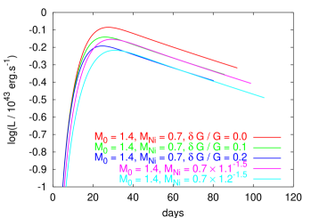
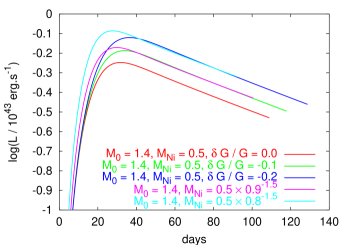
FIG. 5.: Variation of the light curve of SN Ia with respect to an increase of the gravitational constant in the simple “one zone” toy model presented in this article. A stronger gravitational constant accounts for a fainter and narrower light curve (see Eq. (41)). The rising part is mainly sensitive to the progenitor mass whereas the decaying part is mainly dictated by the mass of nickel. Hence each light curve computed with a higher Newton constant tends asymptotically toward the light curve of a supernovae with smaller nickel mass but with standard value of the Newton constant (left), and vice versa (right). [Note that in this last case, we have to ensure that the total nickel mass does not exceed half of the total mass in order for Eq. (39) to be valid.]

3 Application to two examples

In Fig. 6, we show the luminosity distance vs redshift relation for the two models presented above under the assumption that the universe is spatially flat (i.e., $\Omega_{\SS}{\rm mat}+\Omega_{\SS}{\rm Q}=1$). In the case of the nonminimally coupled quintessence field, it can be noted that the deviation is more important for positive $\xi$ than for negative $\xi$. Note that in any case, the net effect of the coupling of the luminosity distance is small (the most extreme values of $\xi$ and $B$ plotted here are already ruled out). However, when fitting the supernovae data, one must also take into account the change in the SN absolute luminosity, which can be as large as $30\%$ for the largest variation of $G$ allowed by nucleosynthesis. We also note that the distance vs redshift relation is more sensitive to the coupling $\xi$ for smaller values of the exponent $\alpha$. From the Friedmann equation (8) and Eq. (5), we have

$${\rm d}\eta\propto F.$$ (49)

Moreover, for constant $\phi$, increasing $\xi$ increases $F$, and therefore the distance traveled by a photon is increased. This explains why the quantity $d_{\SS}{\rm L}-d_{\SS}{\rm L}^{*}$ increases with $\xi$ in Fig. 6. Unfortunately, the same reasoning does not apply for the exponential coupling because the hypothesis that the value of the quintessence field $\phi$ does not significantly vary at fixed redshift when one varies the parameter $B$ is no longer valid. (Should the field be at rest today, then the hypothesis would still be valid, but this is not the case, as shown in Figs. 1 and 3.)

In Fig. 7 we present the distance modulus vs redshift relation taking into account the supernovae luminosity correction due to a variation of the Newton constant. We compare the amplitude of this correction to the standard $\Lambda$CDM model. It appears that the allowed values for $\xi$ do not lead to a significant modification of the distance modulus. This is related to the fact that this model is very strongly constrained by the solar system data. On the contrary, the exponential coupling model allows for a larger deviation of the distance modulus, mainly because it is not limited by the post Newtonian constraints. More generally, any model tuned so to evade the solar system constraints can lead to large deviation in the magnitude vs redshift relation.

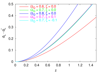
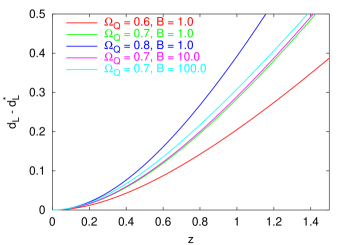
FIG. 6.: Luminosity distance vs redshift relation for different value of $\xi$ (left) and $B$ (right). Both are compared to the luminosity distance vs redshift relation ${\rm d}_{\SS}{\rm L}^{*}$ for a matter dominated, flat universe. As noted previously, the deviation is more important for positive $\xi$ than for negative $\xi$.

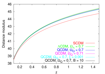
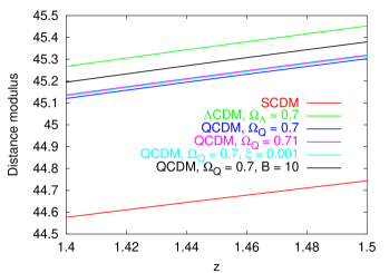
FIG. 7.: Distance modulus vs redshift relation for different models. A comparison between a Standard Cold Dark Matter (SCDM) model, a $\Lambda$CDM model, and a Quintessence Cold Dark Matter (QCDM) model are shown. Also shown are the maximum allowed deviation from a standard QCDM model when considering the two models described in the text. The exponential model allows for large deviations (roughly equivalent to those obtained by adding $\delta\Omega_{\SS}{\rm Q}\sim 0.05$ in a minimally coupled QCDM model), whereas the non minimal coupling is much more constrained. The right panel represents a zoom of the left panel for high redshift.

C Angular distance

Another important observational quantity is the angular distance, ${\rm d}_{\SS}{\rm A}$, which, with the notation of the previous paragraph, is given by [42]

$${\rm d}_{\SS}{\rm A}=\frac{{\rm d}_{\SS}{\rm L}}{(1+z)^{2}}.$$ (50)

This distance relates the size of an object to the angle under which it is observed. Naively, the variation of ${\rm d}_{\SS}{\rm A}$ can be related to the position of the first cosmic microwave background acoustic peak. Note also that ${\rm d}_{\SS}{\rm A}(z)$ also enters the probability of lensing [3].

In Fig. 8, we depict the variation of ${\rm d}_{\SS}{\rm A}(z)$ both in the nonminimally coupled scalar field models and in the exponential coupling case. Indeed, a complete study of the CMB anisotropies will be presented in the following section and these results are just a hint of how the position of the first acoustic peak will be affected in these models. The relative shift in the position of the acoustic peaks is simply given by the asymptotic part of the curves of Fig. 8. As for the luminosity distance, the effect of the coupling is rather small. However, the variation of $G$ will lead to an important modification of the peak position as we shall see later.

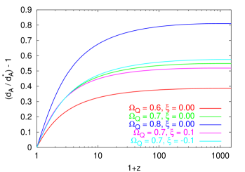
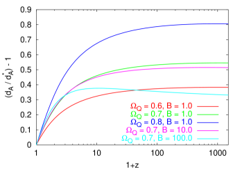
FIG. 8.: Angular distance vs redshift relation for different values of $\xi$ (left) or $B$ (right) compared to $d_{\SS}{\rm A}^{*}$, the angular distance vs redshift relation for a matter dominated, flat universe. The relative shift in the position of the acoustic peaks is simply given by the asymptotic part of the curves. We assumed that $\Omega_{\SS}{\rm Q}=0.7$ and used the SUGRA potential with $\alpha=11$.

III Properties of the perturbations

The background and perturbation equations in a scalar-tensor quintessence model are presented in the appendices. Not that these equations are not restricted to the case of the nonminimally coupled scalar field and can be extended easily to the exponential coupling example by simply setting

$$\xi f=\frac{F(\phi)-1}{2\kappa},$$ (51)

since, as emphasized in the Introduction the splitting (6) is completely general as long as the function $f$ has not be chosen. Technically, one obtains a set of equations slightly more complicated than in the minimally coupled case, but which can still easily be solved numerically. We shall first discuss the main properties of the scalar field perturbations before turning to cosmic microwave background properties in the next section.

As for the minimally coupled case, one of the main concern is about the choice of initial conditions for the perturbations. It happens that this problem is not relevant since the long wavelength scalar field perturbations follow an attractor for the following reason. First, let us consider the unperturbed and perturbed Klein-Gordon equations

$$\ddot{\phi}+2{\cal H}\dot{\phi}+a^{2}V^{\prime} = -\xi a^{2}Rf^{\prime},$$ (52)

$$\ddot{\delta\phi}-\Delta\delta\phi+2{\cal H}\dot{\delta\phi}+a^{2}V^{\prime\prime}\delta\phi-2{\rm X}\ddot{\phi}+\dot{\phi}\left[\Delta\frac{\Phi}{{\cal H}}-\dot{\rm X}-4{\cal H}{\rm X}\right] = -\xi(a^{2}Rf^{\prime\prime}\delta\phi+a^{2}\delta Rf^{\prime}),$$ (53)

where $\Phi$ is one the two Bardeen potential and ${\rm X}$ is a combination of the two Bardeen potentials (see the appendices for more details). For an inverse power law potential, one can show that there exists some particular solution to the unperturbed Klein-Gordon equation, the so-called tracking solution [7], for which the field evolves according to some power law (the exponent of which depends on the exponent of the potential). Then, the stability of this particular solution — which is the most useful feature of the quintessence scenarios — is determined by the properties of the “perturbed” expression of the Klein-Gordon equation. This “perturbed” equation actually describes the small departures of an homogeneous field from its tracking solution, and reads

$$\ddot{\delta\phi}+2{\cal H}\dot{\delta\phi}+a^{2}V^{\prime\prime}\delta\phi=-\xi a^{2}Rf^{\prime\prime}\delta\phi.$$ (54)

Obviously, this equation is extremely similar to the above “real” perturbed Klein-Gordon equation: we simply have neglected the metric perturbation terms, and considered the large wavelength limit $k\to 0$. The very nice feature of inverse power law potential is that the solutions to this equation tend to 0. Therefore, the solutions of the homogeneous part of the real perturbed Klein-Gordon equation in the large wavelength limit tend to 0. Now, when one takes into account the metric perturbations, remembering the fact that they are constant in the long wavelength limit (see, e.g., Ref. [49]), it appears that the relevant quantities, such as $\delta_{\SS}{\rm MC}$ (the density contrast of the quintessence fluid) will tend toward constants which will simply be linear combinations of the metric perturbations. Although not explicitly stated, this is what was shown in Ref. [37]. Finally, in the short wavelength limit, the Laplacian term ensure that the field follows a wave equation, which is actually damped by the expansion.

As a conclusion, as long as the field is subdominant (which is the case when one fixes the initial conditions and in the tracking regimes), its perturbations follow an attractor, thus solving the problem of the choice of the initial conditions, and the field does not show any unstable behavior, as illustrated in Fig. 9.

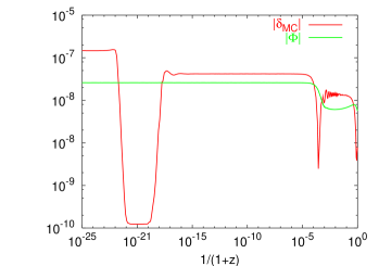
FIG. 9.: Evolution of the scalar field density contrast as a function of redshift for a non minimally quintessence model (SUGRA potential with $\alpha=11$, power law coupling, and $\xi=0.06$). We have represented the evolution of the Fourier mode of the quantity $\delta^{\flat}_{\SS}{\rm MC}(k,z)$ for the wave number $k=0.1h\,{\mbox{Mpc}^{-1}}$. By comparison, we have also shown the Bardeen potential $\Phi$. The quintessence field reaches the attractor around $z\sim 10^{17}$. After this epoch, the quintessence density contrast reaches a value depending only of the potentials $\Phi$ and $\Psi$. It subsequently evolves only when the mode has entered into the Hubble radius, where it experiences damped oscillations (after $z\sim 10^{5}$) around another value also depending on $\Phi$ and $\Psi$. The quintessence density contrast can be very large before having reached the attractor. This is, however, not a problem, because the quintessence density contrast $\Omega_{\SS}{\rm MC}$ is small at this epoch. Note that the Bardeen potential has a nontrivial behavior at late times both because of the domination of the quintessence field (which explains the decay after $z\sim 3$) and because of the variation of the Newton constant.

IV Cosmic microwave background and matter power spectrum

Appendix C gives the derivation of the modified equations for the evolution of the cosmological perturbations. As explained in this appendix, the two most important modifications induced by the quintessence field are (i) a modification of the background equations which lead to the domination of the scalar field today and (ii) a subsequent modification of the late time evolution of the gravitational potentials. We have implemented the scalar-tensor quintessence equations in a Boltzmann code (which uses the line-of-sight integration method, see, e.g., Refs. [50, 51]) and computed matter power spectra as well as CMB anisotropies. We shall now discuss the observable consequences of these models.

Two effects of a quintessence (minimally coupled or not) have already widely been discussed in the literature [37, 52]. These are the following:

• a modification of the angular scale of the peak structure: By modifying the expansion rate of the Universe at low redshift, the quintessence modifies the usual angular distance vs redshift relation (see Fig. 8). This induces a global shift of the acoustic peak structure. Of course, if one adds a quintessence field while keeping fixed the Hubble parameter today, then this is equivalent to modifying the redshift of equivalence between matter and radiation, which of course has some influence of the acoustic peak structure (the same problem occurs for a cosmological constant). From Fig. 8, we would have expected the first acoustic peak to be shifted to smaller multipoles since the diameter angular distance is smaller when $\xi>0$. This is indeed not what is observed on Fig. 11. This is because another, more important effect is that a variation of $G$ modifies the Friedmann equation at early times, and therefore the age of the Universe (and, hence, the sound horizon) is modified. For example, when $\xi>0$, $G$ is larger at earlier time (see Fig. 1), and the age of the Universe is smaller at recombination, which shifts the peak structure towards higher angular scales.

• a boost of the Sachs-Wolfe plateau: When the field starts to dominate, the density parameter of the ordinary matter decay, as well as the gravitational potential. This leads to the possibility of energy exchanges between photons and gravitational field, hence producing the so-called Integrated Sachs-Wolfe (ISW) effect which will boost the anisotropy spectrum of scales larger than the Hubble radius at the epoch of transition between matter and quintessence. The cross correlation between the Sachs-Wolfe and the ISW terms are difficult to compute, and, as long as the ISW term is not too important, one can either have a higher or lower first peak.

For any realistic model, the field is by far subdominant at recombination. As a consequence, the acoustic peak structure of the CMB anisotropies will not directly be affected by the field dynamic. However, two new effects arise when one introduces a non minimally coupled quintessence field:

• a modification of the amplitude of the Silk damping: At small scales, viscosity and heat conduction in the photon-baryon fluid produce a damping of the photon perturbations [51]. The damping scale is determined by the photon diffusion length at recombination, and therefore depends on the size of the horizon at this epoch, and hence, depends on any variation of the Newton constant throughout the history of the Universe.

• a modification of the thickness of the last scattering surface: In the same vein, the duration of recombination is modified by a variation of the Newton constant as the expansion rate is different. It is well known that CMB anisotropies are affected on small scales because the last scattering “surface” has a finite thickness. The net effect is to introduce an extra, roughly exponential, damping term, with the cutoff length being determined by the thickness of the last scattering surface [53]. This thickness is of course determined by the duration of the recombination process. This process is essentially fixed in redshift units, as it is dominated by Boltzmann factors (and hence, by photon temperature) and not by standard cosmological parameters. However, when translating redshift into duration (or length), one has to use the Friedmann equations, which are affected by a variation of the Newton constant. The relevant quantity to consider is the so-called visibility function $g$, defined as

  $$g(\eta)=\dot{\tau}e^{-\tau},$$ (55)

  with $\dot{\tau}$ being the differential opacity, and $\tau|_{\rm today}=0$. In the limit of an infinitely thin last scattering surface, $\tau$ goes from $\infty$ to $0$ at recombination epoch. For standard cosmology, it drops from a large value to a much smaller one, and hence, the visibility function still exhibits a peak, but is much broader. A few examples are given in Fig. 10 for several values of the coupling parameter $\xi$. As it can be seen, the height of the visibility function varies with $\xi$, and therefore, its thickness also varies as the integral of this function is 1.

  

  
  

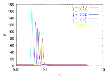
  FIG. 10.: Modification to the visibility function due to non minimal coupling between a quintessence field and curvature. Minimally coupled models are identical to $\Lambda$CDM models since the expansion history of both model is strictly identical at high redshift, whereas important differences can occurs when one introduces a non minimal coupling. For a better readability the various visibility functions have been slightly shifted upward.

• a modification of the sound horizon at recombination: as for the photon diffusion length, the sound horizon depends on the size of the horizon, at can significantly change if the Newton constant is different from now at this epoch. The net effect is to produce a shift in the Doppler peak structure.

More quantitative estimates of all these four effects are difficult to compute analytically, since there is absolutely no reason that there exists any simple solutions to relevant equations. However, as already noted for the supernovae luminosity distance, the effect of the non minimal coupling one the angular size of the acoustic peaks is small, except for unacceptable large value of the parameters. On the contrary, the ISW effect exhibits a much stronger dependence on $\xi$ and $B$, as shown on Fig. 11. One also notices significant modifications in the damping at high multipoles.

On Fig. 12, we have plotted the corresponding matter power spectra. Two important observable effect arise here. First, the normalization of the spectra changes because the usual Sachs-Wolfe formula $\delta T/T=\Phi/3$ which relates the CMB anisotropy to the matter power spectrum amplitudes does no longer hold because of the ISW effect. This is particularly obvious for large, positive values of $\xi$. Second, the maximum of the power spectrum is shifted by the coupling. This is because this maximum give the scale that enters into the Hubble radius at the epoch of equality between matter and radiation. In all the cases presented here, this epoch always corresponds to the same redshift but not to the same cosmic time because the Friedmann equations are modified. Therefore, the relation $H(z)$ is different in all these models.

In practice, the power law coupling (23) is already very strongly constrained by the PN parameters. For all acceptable values of the parameters, the CMB anisotropies show a negligible deviation from the minimally coupled case (note that on Fig. 12, the plotted non zero values of $\xi$ are one order of magnitude larger than allowed values inferred from Fig. 2). On the contrary, for the exponential coupling where the PN constraints are fulfilled by construction, the CMB anisotropies can play a significant role in constraining (or measuring) the coupling parameters.

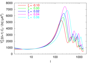
FIG. 11.: Cosmic microwave background anisotropies for the SUGRA potential ($\alpha=11$) with a nonminimally coupled scalar field (left) and with an exponential coupling (right), respectively, for different values of $\xi$ and $B$. We have assume a locally flat Universe. The strongest features are the boost of the decay of the amplitude on large scales due to the Integrated Sachs-Wolfe term, as well as a slight shift of the acoustic peaks structure to higher multipoles.

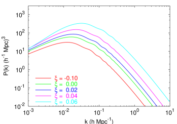
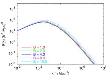
FIG. 12.: Matter power spectrum for the SUGRA potential ($\alpha=11$) with a nonminimally coupled scalar field (left) and with an exponential coupling (right), respectively, for different values of $\xi$ and $B$. We have assumed a locally flat Universe. The unusual features are the variation in the normalization of the power spectra once COBE-normalized, and the shift in the maximum of the spectrum whereas the epoch of equality is the same in all these models.

V Conclusion

In this article, we have investigated the interpretation of cosmological and astrophysical observations in the context of scalar-tensor quintessence. In this class of models, the quintessence field induces a time variation of the gravitational constant and the post-Newtonian constraints and the constraints on the time variation of the constants of nature where first imposed, as well as the restriction arising from nucleosynthesis.

We then focused on the supernovae and cosmic microwave background dataset. Concerning the supernovae, we extracted, using a simple toy model, the dependence of the maximum of the light curve on the gravitational constant. We also explained the various effects of this coupling (mainly the modifications it induces of the Newton constant) on CMB anisotropies and structure formation. All these features on the CMB angular power spectrum and the matter power spectrum are physically well understood.

All these observational constraints were applied all along the article to two class of models: (i) a nonminimally coupled quintessence field and (ii) and exponential coupling. We showed that the first class of models was very constrained mainly because the deviation from the general relativity was fixed and that the constraints were more severe in the case of an inverse power law potential than for the SUGRA potential. The second class seems to leave more freedom for parameters and could possibly be constrained using the CMB.

A Lagrangians

The general action (3) with the ansatz (6) can be decomposed as

$$S=\int\left[{\cal L}_{\SS}{\rm g}+{\cal L}_{\SS}{\rm MC}+{\cal L}_{\SS}{\rm co}+{\cal L}_{\SS}{\rm mat}\right]\sqrt{|g|}{\rm d}^{4}x,$$ (A1)

representing respectively the Lagrangian contribution for the gravity (g), the minimally coupled scalar (MC) field, the coupling (co), and the matter (mat) and given explicitly by

$${\cal L}_{\SS}{\rm g} = -\frac{1}{2\kappa}R,$$ (A2)

$${\cal L}_{\SS}{\rm MC} = \frac{1}{2}g^{\mu\nu}D_{\mu}\phi D_{\nu}\phi-V(\phi),$$ (A3)

$${\cal L}_{\SS}{\rm co} = -\xi Rf(\phi),$$ (A4)

where $D_{\alpha}$ is the covariant derivative of the metric $g_{\alpha\beta}$. By varying the Lagrangian ${\cal L}_{\SS}{\rm Q}$, we obtain the following stress-energy tensor

$$T_{\alpha\beta}^{\SS}{\rm MC}=D_{\alpha}\phi D_{\beta}\phi-\frac{1}{2}D_{\mu}\phi D^{\mu}\phi g_{\alpha\beta}+V(\phi)g_{\alpha\beta}.$$ (A5)

Varying the Lagrangian ${\cal L}_{\SS}{\rm co}$ describing the coupling, one obtains a stress-energy tensor that can be separated into two parts

$$T_{\alpha\beta}^{\SS}{\rm\kappa} = -2\xi G_{\alpha\beta}f,$$ (A6)

$$T_{\alpha\beta}^{\SS}{\rm\xi} = -2\xi\left(g_{\alpha\beta}\Box-D_{\alpha}D_{\beta}\right)f,$$ (A7)

where $G_{\alpha\beta}$ is the Einstein tensor and $\Box\equiv D_{\mu}D^{\mu}$. We have separated the coupling term into two components to single out the part (labeled $\kappa$) which can be absorbed in a redefinition of the Newton constant. It follows that the Einstein equation takes the general form

$$G_{\alpha\beta}=\kappa\sum_{\SS}{f=\SS{\rm MC},\SS{\rm\xi},\SS{\rm\kappa},\SS{\rm mat}}T^{\SS}{f}_{\alpha\beta}$$ (A8)

or, equivalently, with the use of Eq. (5)

$$G_{\alpha\beta}=\kappa_{\SS}{\rm eff}\sum_{\SS}{f=\SS{\rm MC},\SS{\rm\xi},\SS{\rm mat}}T^{\SS}{f}_{\alpha\beta},$$ (A9)

with

$$\kappa_{\SS}{\rm eff}\equiv\frac{\kappa}{F}=\frac{\kappa}{1+2\xi\kappa f}.$$ (A10)

B Background spacetime equations

By varying the Lagrangians with respect to the scalar field, we obtain the Klein-Gordon equation

$$\Box\phi+V^{\prime}=-\xi Rf^{\prime}$$ (B1)

or

$$\ddot{\phi}+2{\cal H}\dot{\phi}+a^{2}V^{\prime}=-\xi a^{2}Rf^{\prime},$$ (B2)

where $R$ stands for the scalar curvature and a prime denotes a derivative with respect to $\phi$. Alternatively, the usual conservation equation ($D_{\mu}T_{\SS}{\rm mat}^{\mu\alpha}=0$) for the matter has to be completed by the conservation equation of each of the stress-energy tensors defined above

$$D_{\mu}T_{\SS}{\rm MC}^{\mu\alpha} = -2\xi[\frac{R}{2}]g^{\mu\alpha}D_{\mu}f\equiv Q^{\alpha}_{\SS}{\rm MC},$$ (B3)

$$D_{\mu}T_{\SS}{\rm\xi}^{\mu\alpha} = -2\xi[-R^{\mu\alpha}]D_{\mu}f\equiv Q^{\alpha}_{\SS}{\rm\xi},$$ (B4)

$$D_{\mu}T_{\SS}{\rm\kappa}^{\mu\alpha} = -2\xi[G^{\mu\alpha}]D_{\mu}f\equiv Q^{\alpha}_{\SS}{\rm\kappa}$$ (B5)

where the $Q^{\nu}$ can be interpreted as a force term [48]. It is straightforward to check that, as expected, the sum of the right-hand sides of these three equations vanishes.

When developing Eq. (A9) with the metric (7), we obtain the Friedmann equations

$$3({\cal H}^{2}+K) = \kappa_{\SS}{\rm eff}a^{2}\sum_{\SS}{f=\SS{\rm mat},\SS{\rm MC},\SS{\rm\xi}}\rho_{\SS}{f},$$ (B6)

$$2({\cal H}^{2}+K-\dot{\cal H}) = -\kappa_{\SS}{\rm eff}a^{2}\sum_{\SS}{f=\SS{\rm mat},\SS{\rm MC},\SS{\rm\xi}}(P_{\SS}{f}+\rho_{\SS}{f}),$$ (B7)

where we have introduced the quantities

$$a^{2}\rho_{\SS}{\rm MC} \equiv \frac{1}{2}\dot{\phi}^{2}+a^{2}V,$$ (B8)

$$a^{2}P_{\SS}{\rm MC} \equiv \frac{1}{2}\dot{\phi}^{2}-a^{2}V,$$ (B9)

$$a^{2}\rho_{\SS}{\rm\xi} \equiv -6\xi{\cal H}\dot{f},$$ (B10)

$$a^{2}P_{\SS}{\rm\xi} \equiv 2\xi(\ddot{f}+{\cal H}\dot{f}).$$ (B11)

$\rho_{\SS}{\rm MC}$ and $P_{\SS}{\rm MC}$ correspond to the minimally coupled part of the scalar field energy density and pressure, $\rho_{\SS}{\rm\xi}$ and $P_{\SS}{\rm\xi}$ to the nonminimally coupled part which can not be absorbed in $\kappa_{\SS}{\rm eff}$. Note that these two equations are not completely straightforward to solve since there are terms proportional to ${\cal H}$, $K$, $\dot{\cal H}$ in $\rho_{\SS}{\rm\xi}$, $P_{\SS}{\rm\xi}$. For example, defining

$${\cal H}_{\SS}{\rm\xi} \equiv \sqrt{-K+\frac{\kappa_{\SS}{\rm eff}a^{2}}{3}\sum_{\SS}{f=\SS{\rm mat},\SS{\rm MC}}\rho_{\SS}{f}},$$ (B12)

$$\epsilon_{\SS}{\rm\xi} \equiv \frac{\xi\dot{f}\kappa_{\SS}{\rm eff}}{{\cal H}_{\SS}{\rm\xi}},$$ (B13)

one gets

$${\cal H}={\cal H}_{\SS}{\rm\xi}\left[\sqrt{1+\epsilon_{\SS}{\rm\xi}}-\epsilon_{\SS}{\rm\xi}\right],$$ (B14)

from which one can compute $\rho_{\SS}{\rm\xi}$. For $P_{\SS}{\rm\xi}$, one can use the following formulas:

$$a^{2}\tilde{P}_{\SS}{\rm\xi} \equiv 2\xi\left[f^{\prime\prime}\dot{\phi}^{2}-{\cal H}f^{\prime}\dot{\phi}-a^{2}V^{\prime}f^{\prime}\right],$$ (B15)

$$\beta \equiv 2\xi^{2}f^{\prime}{}^{2}\kappa_{\SS}{\rm eff},$$ (B16)

$$P_{\SS}{\rm\xi} = \tilde{P}_{\SS}{\rm\xi}+\frac{\beta}{1+3\beta}\left[\rho_{\SS}{\rm\xi}-3\tilde{P}_{\SS}{\rm\xi}+\sum_{\SS}{f=\SS{\rm mat},\SS{\rm MC}}(\rho_{\SS}{f}-3P_{\SS}{f})\right].$$ (B17)

We also set

$$\rho_{\SS}{\rm Q} \equiv \rho_{\SS}{\rm MC}+\rho_{\SS}{\rm\xi},$$ (B18)

$$P_{\SS}{\rm Q} \equiv P_{\SS}{\rm MC}+P_{\SS}{\rm\xi},$$ (B19)

which are the contribution of the scalar field entering the right-hand side of the Friedmann equations, and

$$a^{2}\rho_{\SS}{\rm\kappa} \equiv -6\xi\left({\cal H}^{2}+K\right)f,$$ (B20)

$$a^{2}P_{\SS}{\rm\kappa} \equiv 2\xi\left(2\dot{\cal H}+{\cal H}^{2}+K\right)f,$$ (B21)

which are the quantities entering the redefinition of $\kappa$. With these notations, the conservation equations (B3)–(B5) take the form

$$\dot{\rho}_{\SS}{\rm MC}+3{\cal H}\left(\rho_{\SS}{\rm MC}+P_{\SS}{\rm MC}\right) = -\frac{6\xi\dot{f}}{a^{2}}\left[{\cal H}^{2}+K+\dot{\cal H}\right],$$ (B22)

$$\dot{\rho}_{\SS}{\rm\xi}+3{\cal H}\left(\rho_{\SS}{\rm\xi}+P_{\SS}{\rm\xi}\right) = \frac{6\xi\dot{f}}{a^{2}}[\dot{\cal H}],$$ (B23)

$$\dot{\rho}_{\SS}{\rm\kappa}+3{\cal H}\left(\rho_{\SS}{\rm\kappa}+P_{\SS}{\rm\kappa}\right) = \frac{6\xi\dot{f}}{a^{2}}\left[{\cal H}^{2}+K\right],$$ (B24)

and it can be checked, as expected, that the sum of the right-hand sides of Eqs. (B22)–(B24) vanishes.

In practice, it is not difficult to solve this set of equations [apart from the subtleties described in Eqs. (B12)–(B17)]. The main problem arises from the fact that we know a priori neither the values of the energy scale of the potential (1),(2), nor the bare Einstein constant $\kappa$. All what we know (or impose) are the value of $\Omega_{\SS}{\rm Q}$ and $\kappa_{\SS}{\rm eff}$ today. We are therefore obliged to use standard routines [54] to find a solution that converges towards the desired values for $\Omega_{\SS}{\rm Q}$ and $\kappa_{\SS}{\rm eff}$ today. In order to do so, one is obliged to provide a reasonably good starting point for $\kappa$ and $M$. In practice, one can consider

$$\kappa_{\SS}{\rm start} = 8\pi G,$$ (B25)

$$M_{\SS}{\rm start} = (\rho_{\SS}{\rm crit}M_{\SS}{\rm Pl}^{\alpha})^{\frac{1}{4+\alpha}},$$ (B26)

which usually converges for reasonable values of the parameters. When this starting point fails to converge, we are usually in a region of the parameter space already ruled out by the astrophysical constraints detailed in Sec. II A.

C Perturbation equations

We consider the general form of a perturbed cosmological spacetime

$${\rm d}s^{2}=a^{2}\left[(1+2A){\rm d}\eta^{2}+2(\nabla_{i}B+\overline{B}_{i}){\rm d}\eta{\rm d}x^{i}-(\gamma_{ij}+2C\gamma_{ij}+2\nabla_{i}\nabla_{j}E+2\nabla_{(i}\overline{E}_{i)}+2\overline{\overline{E}}_{ij}){\rm d}x^{i}{\rm d}x^{j}\right],$$ (C1)

where $\gamma_{ij}$ is the metric of the homogeneous spatial sections and $\nabla_{i}$ its covariant derivative. The vector quantities $\overline{B}_{i}$ and $\overline{E}_{i}$ are divergenceless ($\nabla^{i}\overline{B}_{i}=\nabla^{i}\overline{E}_{i}=0$), and the tensor $\overline{\overline{E}}_{ij}$ is divergenceless and traceless.

For any fluid, the stress-energy tensor can be decomposed as

$$T_{\alpha\beta}=(P+\rho)u_{\alpha}u_{\beta}-Pg_{\alpha\beta}+\Pi_{\alpha\beta},$$ (C2)

where $\Pi_{\alpha\beta}$ is a traceless tensor orthogonal the the four-velocity $u^{\alpha}$. For a perfect fluid, we have $\Pi_{\alpha\beta}=0$. We then define

$$-a^{2}(P+\rho)v_{i} \equiv (P+\rho)u_{0}g_{ij}\delta u^{j}+\delta\Pi_{0i},$$ (C3)

$$a^{2}P\pi_{ij} \equiv \delta\Pi_{ij},$$ (C4)

where $v_{i}$ and $\pi_{ij}$ have to be seen as three-dimensional quantities whose indices are raised and lowered by the metric $\gamma_{ij}$. Using these quantities, the stress-energy tensor perturbation takes the form

$$\delta T_{00} = \rho a^{2}\left(\delta+2A\right),$$ (C5)

$$\delta T_{0i} = \rho a^{2}\left[\nabla_{i}B+\overline{B}_{i}-(1+\omega)(\nabla_{i}v+\overline{v}_{i})\right],$$ (C6)

$$\delta T_{ij} = Pa^{2}\left[h_{ij}+\frac{\delta P}{P}\gamma_{ij}+\Delta_{ij}\pi+D_{(i}\overline{\pi}_{j)}+\overline{\overline{\pi}}_{ij}\right],$$ (C7)

where $h_{ij}\equiv 2C\gamma_{ij}+2\nabla_{i}\nabla_{j}E+2\nabla_{(i}\overline{E}_{i)}+2\overline{\overline{E}}_{ij}$, $\Delta_{ij}\equiv\nabla_{i}\nabla_{j}-\gamma_{ij}\Delta/3$, $\Delta\equiv\nabla_{i}\nabla^{i}$ being the Laplacian, and $\pi$, $\overline{\pi}_{i}$ and $\overline{\overline{\pi}}_{ij}$ are the scalar, vector and tensor components of the anisotropic stress tensor.

We work in the gauge in which $B=E=0$ and $\overline{E}_{i}=0$ and introduce the gauge invariant perturbation variables, labeled with a superscript $\sharp$,

$$\delta^{\sharp} \equiv \frac{\delta\rho}{\rho}-\frac{\dot{\rho}}{\rho}(B+\dot{E}),$$ (C8)

$$v^{\sharp} \equiv v+\dot{E},$$ (C9)

$$\overline{v}^{\sharp}_{i} \equiv \overline{v}_{i}+\dot{\overline{E}}_{i},$$ (C10)

and the four gauge invariant gravitational potentials

$$\Psi \equiv A+{\cal H}(B+\dot{E})-(\dot{B}+\ddot{E}),$$ (C11)

$$\Phi \equiv -C+{\cal H}(B+\dot{E}),$$ (C12)

$${\rm X} \equiv A-C-\frac{\partial}{\partial\eta}\left(\frac{C}{{\cal H}}\right),$$ (C13)

$$\overline{V}_{i} \equiv \overline{B}_{i}+\dot{\overline{E}}_{i}.$$ (C14)

(Note that ${\rm X}$ can be expressed in terms of $\Phi$ and $\Psi$ and their time derivatives. It will, however, prove useful to work with these three quantities.) The pressure perturbations are related to the density contrasts by

$$\frac{\delta P^{\sharp}}{P}=\frac{c_{s}^{2}}{\omega}{\delta^{\sharp}}+\Gamma,$$ (C15)

where $c_{s}^{2}=\dot{P}/\dot{\rho}$ is the (adiabatic) sound speed and $\Gamma$ is the entropy perturbation. As we shall see later, $\Gamma_{\SS}{\rm\xi}$ and $\Gamma_{\SS}{\rm MC}$ do not vanish. We also introduce the convenient flat-slicing gauge in which $C=E=0$ and $\overline{E}_{i}=0$ (and thus where $A={\rm X}$ and $B=\Phi/{\cal H}$) and where the gauge invariant density contrast and pressure perturbations, labeled with a superscript $\flat$, are given by

$$\delta^{\flat} \equiv \frac{\delta\rho}{\rho}-\frac{\dot{\rho}}{\rho}\frac{C}{{\cal H}}=\delta^{\sharp}+\frac{\dot{\rho}}{\rho}\frac{\Psi}{{\cal H}},$$ (C16)

$$\frac{\delta P^{\flat}}{P} = \frac{\delta P^{\sharp}}{P}+\frac{\dot{P}}{P}\frac{\Psi}{{\cal H}}.$$ (C17)

Note that in Eq. (C16) we do not use the conservation equation to express $\dot{\rho}$ in order for this definition to be valid also for coupled fluids. The velocity perturbations are identical in both gauges.

The scalar field is decomposed as $\phi(\eta)+\delta\phi$ and we introduce the two gauge invariant variables, respectively, in Newtonian and flat-slicing gauge

$$\delta\phi^{\sharp} \equiv \delta\phi-\dot{\phi}(B+\dot{E}),$$ (C18)

$$\delta\phi^{\flat} \equiv \delta\phi^{\sharp}+\dot{\phi}\frac{\Phi}{{\cal H}}.$$ (C19)

It is indeed not the purpose of this Appendix to rederive all the equations of perturbation; our aim is to take into account the nonminimally coupled scalar field. For that purpose, we first compute Klein-Gordon equation. Then, we compute the perturbed stress-energy tensor to deduce the Einstein equations, using the standard scalar-vector-tensor decomposition.

1 Perturbed Klein-Gordon equation

The perturbed Klein-Gordon equation reduces to

$$\ddot{\delta\phi}^{\flat}-\Delta\delta\phi^{\flat}+2{\cal H}\dot{\delta\phi}^{\flat}+a^{2}V^{\prime\prime}\delta\phi^{\flat}-2{\rm X}\ddot{\phi}+\dot{\phi}\left[\Delta\frac{\Phi}{{\cal H}}-\dot{\rm X}-4{\cal H}{\rm X}\right]=-\xi(a^{2}Rf^{\prime\prime}\delta\phi^{\flat}+a^{2}\delta R^{\flat}f^{\prime}),$$ (C20)

where we have used the scalar curvature $R$

$$a^{2}R=-6({\cal H}^{2}+K+\dot{\cal H}),$$ (C21)

and of its perturbation $\delta R^{\flat}$, in the flat-slicing gauge

$$a^{2}\delta R^{\flat}=2\Delta(\Psi-2\Phi)+6(2{\cal H}^{2}{\rm X}+2\dot{\cal H}{\rm X}+{\cal H}\dot{\rm X}).$$ (C22)

2 Perturbed fluid quantities

After some manipulations, it appears that it is possible to arrange the stress-energy tensor $T_{\alpha\beta}^{\SS}{\rm MC}$ so that a minimally coupled scalar field essentially behaves similar to a fluid:

$$\rho_{\SS}{\rm MC} = \frac{1}{2}D_{\mu}\phi D^{\mu}\phi+V,$$ (C23)

$$P_{\SS}{\rm MC} = \frac{1}{2}D_{\mu}\phi D^{\mu}\phi-V,$$ (C24)

$$u_{\SS}{\rm MC}^{\alpha} = \frac{D^{\alpha}\phi}{\sqrt{D_{\mu}\phi D^{\mu}\phi}},$$ (C25)

$$\Pi_{\SS}{\rm MC}^{\alpha\beta} = 0.$$ (C26)

From these expressions, it is then possible to compute density and pressure perturbations, etc.,

$$a^{2}\delta\rho_{\SS}{\rm MC}^{\flat} = \dot{\phi}\dot{\delta\phi}^{\flat}+a^{2}V^{\prime}\delta\phi^{\flat}+\dot{\phi}^{2}{\rm X},$$ (C27)

$$a^{2}\delta P_{\SS}{\rm MC}^{\flat} = \dot{\phi}\dot{\delta\phi}^{\flat}-a^{2}V^{\prime}\delta\phi^{\flat}+\dot{\phi}^{2}{\rm X},$$ (C28)

$$a^{2}(P_{\SS}{\rm MC}+\rho_{\SS}{\rm MC})v^{\flat}_{\SS}{\rm MC} = -\dot{\phi}\delta\phi^{\flat}+\dot{\phi}^{2}\frac{\Phi}{{\cal H}},$$ (C29)

$$a^{2}(P_{\SS}{\rm MC}+\rho_{\SS}{\rm MC})\overline{v}^{\flat}_{\SS{\rm MC}\;i} = \dot{\phi}^{2}\overline{V}_{i},$$ (C30)

$$a^{2}P_{\SS}{\rm MC}\pi_{ij}^{\SS}{\rm MC} = 0.$$ (C31)

Similar expressions can be found for the $\xi$ part. For the density and the pressure, we have

$$\rho_{\SS}{\rm\xi} = \frac{1}{4}(-6\xi\Box f+3\sqrt{Y}),$$ (C32)

$$P_{\SS}{\rm\xi} = \frac{1}{4}(6\xi\Box f+\sqrt{Y}),$$ (C33)

with

$$Y=\frac{1}{3}\left[4T^{\SS}{\rm\xi}_{\mu\nu}T_{\SS}{\rm\xi}^{\mu\nu}-(g_{\mu\nu}T_{\SS}{\rm\xi}^{\mu\nu})^{2}\right]=\left[\frac{2\xi}{a^{2}}(\ddot{f}-2{\cal H}\dot{f})\right]^{2}.$$ (C34)

As for the minimally coupled part, we set

$$u_{\SS}{\rm\xi}^{\alpha}=\frac{D^{\alpha}f}{\sqrt{D_{\mu}fD^{\mu}f}},$$ (C35)

from which we deduce an anisotropic stress $\Pi_{\SS}{\rm\xi}^{\alpha\beta}$:

$$\Pi_{\SS}{\rm\xi}^{\alpha\beta}=[T_{\SS}{\rm\xi}^{\alpha\beta}-\frac{1}{4}g^{\alpha\beta}T_{\SS}{\rm\xi}^{\mu\nu}g_{\mu\nu}]-\sqrt{Y}\left(u_{\SS}{\rm\xi}^{\alpha}u_{\SS}{\rm\xi}^{\beta}-\frac{1}{4}g^{\alpha\beta}\right).$$ (C36)

One can easily check that $\Pi_{\SS}{\rm\xi}^{\alpha\beta}=0$ and $\delta\Pi_{\SS}{\rm\xi}^{00}=0$. Using Eqs. (C3),(C4),(C6),(C7), we finally obtain

$$a^{2}\delta\rho_{\SS}{\rm\xi}^{\flat} = 2\xi\left[-3{\cal H}\dot{\delta f}^{\flat}+6{\cal H}\dot{f}X+\Delta\left(\delta f^{\flat}-\dot{f}\frac{\Phi}{{\cal H}}\right)\right],$$ (C37)

$$a^{2}\delta P_{\SS}{\rm\xi}^{\flat} = 2\xi\left[\ddot{\delta}f^{\flat}+{\cal H}\dot{\delta f}^{\flat}-\frac{2}{3}\Delta\left(\delta f^{\flat}-\dot{f}\frac{\Phi}{{\cal H}}\right)-\dot{f}\dot{\rm X}-2\ddot{f}{\rm X}-2{\cal H}\dot{f}{\rm X}\right],$$ (C38)

$$a^{2}(P_{\SS}{\rm\xi}+\rho_{\SS}{\rm\xi})v^{\flat}_{\SS}{\rm\xi} = 2\xi\left[-\dot{\delta f}{}^{\flat}+{\cal H}\delta f^{\flat}+(\ddot{f}-2{\cal H}\dot{f})\frac{\Phi}{{\cal H}}+\dot{f}{\rm X}\right],$$ (C39)

$$a^{2}(P_{\SS}{\rm\xi}+\rho_{\SS}{\rm\xi})\overline{v}^{\flat}_{\SS{\rm\xi}\;i} = 2\xi(\ddot{f}-2{\cal H}f)\overline{V}_{i},$$ (C40)

$$a^{2}P_{\SS}{\rm\xi}\pi^{\SS}{\rm\xi} = -2\xi\left(\dot{f}\frac{\Phi}{{\cal H}}-\delta f^{\flat}\right),$$ (C41)

$$a^{2}P_{\SS}{\rm\xi}\overline{\pi}_{i}^{\SS}{\rm\xi} = -2\xi\dot{f}\overline{V}_{i},$$ (C42)

$$a^{2}P_{\SS}{\rm\xi}\overline{\overline{\pi}}_{ij}^{\SS}{\rm\xi} = -2\xi\dot{f}\dot{\overline{\overline{E}}}_{ij}.$$ (C43)

Finally, the perturbation of $T_{\alpha\beta}^{\SS}{\rm\kappa}$ gives

$$\delta T_{\alpha\beta}^{\SS}{\rm\kappa}=2\xi\delta G_{\alpha\beta}f+2\xi G_{\alpha\beta}\delta f\equiv\delta T_{\alpha\beta}^{\SS{\rm\kappa}_{\SS}{\rm L}}+\delta T_{\alpha\beta}^{\SS{\rm\kappa}_{\SS}{\rm R}}.$$ (C44)

In the next section, we shall inject these results into the Einstein equations.

3 Einstein Equations

With these quantities and the standard expressions of the perturbed Einstein tensor, which can be found, e.g., in Ref. [55], we can give the perturbed Einstein equations

$$\delta G_{\alpha\beta}=\kappa\sum_{\SS}{f=\SS{\rm mat},\SS{\rm\kappa},\SS{\rm\xi},\SS{\rm MC}}\delta T_{\alpha\beta}^{\SS}{f}\Longleftrightarrow\delta G_{\alpha\beta}=\kappa_{\SS}{\rm eff}\sum_{\SS}{f=\SS{\rm mat},\SS{\rm\kappa}_{\SS}{\rm R},\SS{\rm\xi},\SS{\rm MC}}\delta T_{\alpha\beta}^{\SS}{f}$$ (C45)

in the scalar-vector-tensor decomposition.

a Scalar modes

After some long but straightforward manipulations, we finally obtain

$$2(\Delta\Phi-3{\cal H}^{2}{\rm X}) = 3{\cal H}^{2}\sum_{\SS}{f=\SS{\rm mat},\SS{\rm\xi},\SS{\rm MC}}\Omega_{\SS}{f}\left(\delta^{\flat}_{\SS}{f}+\frac{\delta\kappa_{\SS}{\rm eff}^{\flat}}{\kappa_{\SS}{\rm eff}}\right),$$ (C46)

$$-2\left[{\cal H}^{2}{\rm X}+\left(\dot{\cal H}-{\cal H}^{2}\right)\Phi\right] = 3{\cal H}^{2}\sum_{\SS}{f=\SS{\rm mat},\SS{\rm\xi},\SS{\rm MC}}\Omega_{\SS}{f}(1+\omega_{\SS}{f}){\cal H}v^{\flat}_{\SS}{f},$$ (C47)

$$\Phi-\Psi = 3{\cal H}^{2}\sum_{\SS}{f=\SS{\rm mat},\SS{\rm\xi},\SS{\rm MC}}\Omega_{\SS}{f}\omega_{\SS}{f}\pi_{\SS}{f},$$ (C48)

$$2\left[{\cal H}^{2}{\rm X}+2\dot{\cal H}{\rm X}+{\cal H}\dot{\rm X}+\frac{1}{3}\Delta(\Psi-\Phi)\right] = 3{\cal H}^{2}\sum_{\SS}{f=\SS{\rm mat},\SS{\rm\xi},\SS{\rm MC}}\Omega_{\SS}{f}\omega_{\SS}{f}\left(\frac{\delta P^{\flat}_{\SS}{f}}{P_{\SS}{f}}+\frac{\delta\kappa_{\SS}{\rm eff}^{\flat}}{\kappa_{\SS}{\rm eff}}\right).$$ (C49)

We therefore end with a linear system relating the four metric perturbations $\Phi$, $\Psi$, ${\rm X}$, $\dot{\rm X}$ to the fluid perturbed quantities, some of which depending on the metric perturbations, [cf Eqs. (C27)–(C43)]. This system can easily be solved numerically in order to extract the metric perturbations, which in turn source the perturbed mass conservation, and Euler and Klein-Gordon equations. Apart from the different expressions for the metric perturbations, the other fluid conservation equation are not modified by the presence of the quintessence field. Hence it is quite straightforward to implement this in any preexisting numerical code.

b Vector modes

In the same way, we obtain

$$\left[-\frac{1}{2}(\Delta+2K)+2({\cal H}^{2}+K-\dot{\cal H})\right]\overline{V}_{i} = 3{\cal H}^{2}\sum_{\SS}{f=\SS{\rm mat},\SS{\rm\xi},\SS{\rm MC}}\Omega_{\SS}{f}(1+\omega_{\SS}{f}){\cal H}v^{\SS{f}\;\flat}_{i},$$ (C50)

$$2{\cal H}^{2}\overline{V}_{i}+{\cal H}\dot{\overline{V}}_{i} = 3{\cal H}^{2}\sum_{\SS}{f=\SS{\rm mat},\SS{\rm\xi},\SS{\rm MC}}\Omega_{\SS}{f}\omega_{\SS}{f}\overline{\pi}^{\SS}{f}_{i},$$ (C51)

which is then easily solved.

c Tensor modes

The equation of evolution of the gravitational waves reads

$$\ddot{\overline{\overline{E}}}_{ij}+2{\cal H}\dot{\overline{\overline{E}}}_{ij}+(2K-\Delta)\overline{\overline{E}}_{ij}=3{\cal H}^{2}\sum_{\SS}{f=\SS{\rm mat},\SS{\rm\xi},\SS{\rm MC}}\Omega_{\SS}{f}\omega_{\SS}{f}\overline{\overline{\pi}}^{\SS}{f}_{ij}.$$ (C52)

The presence of the term proportional to $\dot{\overline{\overline{E}}}_{ij}$ in Eq. (C43) indicates that the damping rate of the gravitational waves is different. This result is identical to the one we had obtained in an earlier work [13].

REFERENCES

- [1] A.G. Riess et al., “Observational evidence from supernovae for an accelerating universe and a cosmological constant”, Astron. J. 116, 1009 (1998), [astro-ph/9806396]; S. Perlmutter et al., “Discovery of a supernovae explosion at half the age of the universe and its cosmological implications”, Nature391, 51 (1998), [astro-ph/9712212].
- [2] P. de Bernardis et al., “A Flat Universe from High-Resolution Maps of the Cosmic Microwave Background Radiation”, Nature404, 955 (2000), [astro-ph/0004404].
- [3] Y. Mellier, Annu. Rev. Astron. Astrophys. 37, 127 (1999).
- [4] S. Weinberg, “The cosmological constant problem”, Rev. Mod. Phys. 61, 1 (1989).
- [5] P. Binétruy, in The Early Universe, proceedings of Les Houches summer school, 1999, “Cosmological constant vs quintessence”, [Int. J. Theor. Phys. 39 1859 (2000)], [hep-ph/0005037].
- [6] S.M. Carroll, “The cosmological constant”, Living Rev. Relativ. 4, 1 (2001), [astro-ph/0004075].
- [7] B. Ratra and P.J.E. Peebles, “Cosmological consequences of a rolling homogeneous scalar field”, Phys. Rev. D37, 3406 (1988).
- [8] C.Wetterich, “Cosmology and the fate of dilatation symmetry”, Nucl. Phy. B302, 668 (1988).
- [9] R.R. Caldwell, R. Dave, and P.J. Steinhardt, “Cosmological imprint of an energy component with general equation of state”, Phys. Rev. Lett.80, 1582 (1998), [astro-ph/9708069].
- [10] P. Binétruy, “Models of dynamical supersymmetry breaking and quintessence”, Phys. Rev. D60, 063502 (1999), [hep-th/9810553].
- [11] P. Brax and J. Martin, “The robustness of quintessence”, Phys. Rev. D61, 103502 (2000), [astro-ph/9912046].
- [12] I. Zlatev, L. Wang, and P.J. Steinhardt, “Quintessence, Cosmic Coincidence, and the Cosmological Constant”, Phys. Rev. Lett.82, 896 (1999), [astro-ph/9807002].
- [13] A. Riazuelo and J.–P. Uzan, “Quintessence and Gravitational Waves”, Phys. Rev. D62, 083506 (2000), [astro-ph/0004156].
- [14] K. Benabed and F. Bernardeau, “Testing quintessence models with large-scale structure growth”, Phys. Rev. D64, 083501 (2001), [astro-ph/0104371].
- [15] S.M. Carroll, Phys. Rev. Lett.81, 3067 (1998).
- [16] P. Brax and J. Martin, “Quintessence and Supergravity”, Phys. Lett. B 468, 40 (1999), [astro-ph/9905040].
- [17] M.B. Green, J.H. Schwarz, and E. Witten, Superstring Theory (Cambridge University Press, Cambridge, England, 1987).
- [18] N. Banerjee and D. Pavon, “A quintessence scalar field in Brans-Dicke theory”, Class. Quantum Grav. 18, 593 (2001), [gr-qc/0012098].
- [19] J.–P. Uzan, “Cosmological scaling solutions of nonminimally coupled scalar fields”, Phys. Rev. D59, 123510 (1999), [gr-qc/9903004].
- [20] L. Amendola, “Coupled Quintessence”, Phys. Rev. D62, 043511 (2000), [astro-ph/9908023].
- [21] F. Perrotta, C. Baccigalupi, and S. Matarrese, “Extended Quintessence”, Phys. Rev. D61, 023507 (2000), [astro-ph/9906066].
- [22] G. Esposito-Farèse and D. Polarski, “Scalar-tensor gravity in an accelerating universe”, Phys. Rev. D63, 063504 (2001), [gr-qc/0009034].
- [23] C.M. Will, Theory and Experiments in Gravitational Physics (Cambridge University Press, Cambridge, England, 1993).
- [24] D. Wands, “Extended Gravity Theories and the Einstein-Hilbert Action”, Class. Quantum Grav. 11, 269 (1994), [gr-qc/9307034].
- [25] T. Damour and G. Esposito-Farèse, “Tensor multi-scalar theories of gravitation”, Class. Quantum Grav. 9, 2093 (1992).
- [26] L. Amendola, “Scaling solutions in general nonminimal coupling theories”, Phys. Rev. D60, 043501 (1999), [astro-ph/9904120].
- [27] R. de Ritis, A.A. Marino, C. Rubano, and P. Scudellaro, “Tracker fields from nonminimally coupled theory”, Phys. Rev. D62, 043506 (2000), [hep-th/9907198].
- [28] O. Bertolami and P.J. Martins, “Nonminimal coupling and quintessence”, Phys. Rev. D61, 064007 (2000), [gr-qc/9910056].
- [29] T. Chiba, “Quintessence, the Gravitational Constant, and Gravity”, Phys. Rev. D60, 083508 (1999), [gr-qc/9903094].
- [30] N. Bartolo and M. Pietroni, “Scalar Tensor gravity and quintessence”, Phys. Rev. D61, 023518 (2000), [hep-ph/9908521].
- [31] T. Damour and K. Nordtvedt, “Tensor-scalar cosmological models and their relaxation toward general relativity”, Phys. Rev. D48, 3436 (1993).
- [32] X. Chen and M. Kamionkowsky, “Cosmic Microwave Background Temperature and Polarization Anisotropy in Brans-Dicke Cosmology”, Phys. Rev. D60, 104036 (1999), [astro-ph/9905368].
- [33] C. Baccigaluppi, S. Matarrese, and F. Perrotta, “Tracking Extended Quintessence”, Phys. Rev. D62, 123510 (2000), [astro-ph/0005543].
- [34] L. Amendola, “perturbations in a coupled scalar field cosmology”, Month. Not. R. Astron. Soc. 312, 521 (2000), [astro-ph/9906073].
- [35] L. Amendola, “Dark energy and the Boomerang data”, Phys. Rev. Lett.86, 196 (2001), [astro-ph/0006300].
- [36] X. Chen, R.J. Scherrer, and G. Steigman, “Extended quintessence and the primordial helium abundance”, Phys. Rev. D63, 123504 (2001), [astro-ph0011531].
- [37] P. Brax, J. Martin, and A. Riazuelo, “Exhaustive Study of Cosmic Microwave Background Anisotropies in Quintessential Scenarios”, Phys. Rev. D62, 103505 (2000), [astro-ph/0005428].
- [38] C. Will, “The Confrontation between General Relativity and Experiment”, Living Rev. Rel. 4, 4 (2001), [gr-qc/0103036].
- [39] J.O. Dickey et al., Science 265, 482 (1994).
- [40] P.G. Ferreira and M. Joyce, “Cosmology with a Primordial Scaling Field”, Phys. Rev. D58, 023503 (1998), [astro-ph/9711102].
- [41] T. Damour and B. Pichon, “Big Bang nucleosynthesis and scalar-tensor gravity”, Phys. Rev. D59, 104036 (1999), [astro-ph/9807176].
- [42] P.J.E. Peebles, Principles of Physical Cosmology (Princeton University Press, Princeton, 1993).
- [43] E. Garcia-Berro et al., “On the Evolution of Cosmological Type Ia Supernovae and the Gravitational Constant”, [astro-ph/9907440].
- [44] D. Arnett, Supernovae and Nucleosynthesis (Princeton university Press, Princeton, 1996).
- [45] R. Mochkovitch, in Matter under Extreme Conditions, edited by H. Latal and W. Schweiger (Springer Verlag, Berlin, 1994) p. 49.
- [46] L. Amendola, S. Corasaniti, and F. Occhionero, “Time variability of the gravitational constant and Type Ia supernovae”, [astro-ph/9907222].
- [47] B. Boisseau, G. Esposito-Farèse, D. Polarski, and A.A. Starobinsky, Phys. Rev. Lett.85, 2236 (2000).
- [48] J.–P. Uzan, “Dynamics of relativistic interacting gases: from a kinetic to a fluid description”, Class. Quantum Grav. 15, 1063 (1998), [gr-qc/9801108].
- [49] E. Bunn, in The Cosmic Microwave Background, edited by C. Lineweaver et al. (Kluwer, Dordrecht, 1997) p. 135.
- [50] U. Seljak and M. Zaldarriaga, “A line-of-sight integration approach to cosmic microwave background anisotropies”, ApJ469, 444 (1996), [astro-ph/9603033].
- [51] W. Hu and M. White, “CMB anisotropies: total angular momentum method”, Phys. Rev. D56, 596 (1997), [astro-ph/9702170].
- [52] F. Perrotta, C. Baccigalupi, and S. Matarrese, “Extended quintessence”, Phys. Rev. D61, 023507 (2000), [astro-ph/9906066]; C. Baccigalupi, S. Matarrese and F. Perrotta, “Tracking extended quintessence”, ibid. 62, 123510 (2000), [astro-ph/0005543].
- [53] U. Seljak, “A two fluid approximation for calculating the cosmic microwave background anisotropies”, ApJLett. 435, L87 (1994), [astro-ph/9406050].
- [54] W. Press et al., Numerical recipes in C, 2nd. ed. (Cambridge University Press, Cambridge, England, 1992).
- [55] H. Kodama and M. Sasaki, “Cosmological perturbation theory”, Prog. Theor. Phys. Suppl. 78, 1 (1984); V. Mukhanov, H. Feldman and R. Brandenberger, “Theory of cosmological perturbations”, Phys. Rep. 215, 203 (1992); R. Durrer, “Gauge invariant cosmological perturbation theory: a general study and its application to the texture scenario of structure formation”, Fundam. Cosmic Phys. 14, 209 (1994).