Fast Clustering Analysis of Inhomogenous Megapixel CMB Maps

Abstract

Szapudi et al. (2001) introduced the method of estimating angular power spectrum of the CMB sky via heuristically weighted correlation functions. Part of the new technique is that all (co)variances are evaluated by massive Monte Carlo simulations, therefore a fast way to measure correlation functions in a high resolution map is essential. This letter presents a new algorithm to calculate pixel space correlation functions via fast spherical harmonics transforms. Our present implementation of the idea extracts correlations from a MAP-like CMB map (HEALPix resolution of $512$, i.e. $\simeq 3\times 10^{6}$ pixels) in about 5 minutes on a 500MHz computer, including $C_{\ell}$ inversion; the analysis of one Planck-like map takes less then one hour. We use heuristic window and noise weighting in pixel space, and include the possibility of additional signal weighting as well, either in $\ell$ or pixel space. We apply the new code to an ensemble of MAP simulations, to test the response of our method to the inhomogenous sky coverage/noise of MAP. We show that the resulting $C_{\ell}$’s are very close to the theoretical expectations. The HEALPix based implementation of the method, SpICE (Spatially Inhomogenous Correlation Estimator) will be available to the public from the authors.

1 Introduction

With the successful launch of MAP and the advancing Planck schedule, megapixel Cosmic Microwave Background (CMB) maps are just around the corner. To fully realize their potential of constraining cosmological parameters within a few percent (e.g., Spergel 1994; Knox 1995; Hinshaw, Bennett, & Kogut 1995; Jungman et al. 1996; Zaldarriaga, Spergel & Seljak 1997; Bond, Efstathiou, & Tegmark 1997), data analysis methods have to face hitherto unprecedented challenges. The standard maximum likelihood developed for COBE (e.g., Górski 1994; Górski et al. 1994, 1996; Bond 1995; Tegmark & Bunn 1995; Tegmark 1996; Bunn & White 1996; Bond, Jaffe, & Knox 1998, 2000) is already pushing supercomputers for balloon-borne and ground based experiments with $N\simeq 10^{5}$ pixels (de Bernardis et al. 2000; Netterfield et al. 2001; Hanany et al. 2000; Jaffe et al. 2000; Martin et al. 1996; Miller et al. 1999; Peterson et al. 2000), and it is clearly inadequate for analysing megapixel maps on any future supercomputer. This letter addresses an important step in the full data processing pipeline from component separation/mapmaking to cosmological parameter estimation: the fast estimation of the angular power spectrum, $C_{\ell}$ from megapixel map with realistic geometry (sky cut, cut out holes), and inhomogeneous coverage and noise.

A recent surge of activity motivated by the obvious need for fast alternatives to the standard maximum likelihood estimation produced an array of promising techniques. Several of them use symmetries of a particular experiment to gain speed. An experiment specific technique for MAP was developed by Oh, Spergel and Hinshaw (1998) making use of the planned approximate azimuthal symmetry of the coverage/noise. Similar developments are under way for Planck (e.g., Wandelt 2000) possibly exploiting symmetries in its scanning strategy. Other techniques give up optimality in favor of speed. Correlation functions with simple weights were advocated by Szapudi et al. (2001, hereafter SPPSB), while an analogous method based on direct spherical Fourier transform was developed by Hivon et al. (2001). In the standard CMB formalism (e.g. Bond et al. 1998) both of these can be thought of as quadratic estimators with suboptimal weights, yet, they tend to produce results very close to optimal.

This letter presents significant improvements of the correlation function method. We present a fast algorithm for extracting the pixel space estimator using fast spherical harmonics transform, introduce noise weighting, test the use of Monte Carlo realizations to calculate noise correlation functions in the estimator, and finally illustrate the possibility of additional signal weighting.

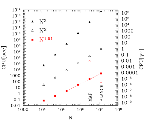
Figure 1: CPU requirements of selected CMB analysis methods are plotted: MADCAP ($N^{3}$, filled triangles, Borrill 1999), SPPSB ($N^{2}$, open triangles), and the present method ($\simeq N^{1.61}$, filled squares). The experiment specific technique of OSH for MAP is plotted with a cross, while an open square illustrates how Moore’s law will shift the CPU for our method by 2007. All the squares are actual measured values on a 500Mhz CPU, while the triangles are based on extrapolation of scaling. The two leftmost points are relevant for MAP and Planck. The righthand $y$-axis displays CPU time in years, instead of seconds for clarity.

2 Summary of the Method

Our latest recipe to extract $C_{\ell}$’s from a large CMB map is an improved version of SPPSB: extract the two-point correlation function with an unbiased weighted estimator sampled at the roots of Legendre polynomials, then integrate with a Gauss-Legendre quadrature to obtain the $C_{\ell}$’s. Next we review the correlation function estimator.

Let us denote the temperature fluctuations at a sky vector $n$, a unit vector pointing to a pixel on the sky, with $T(n)$. In isotropic universes the two-point correlation function is a function only of the angle between the two vectors and can expanded into a Legendre series,

$$\xi_{12}=\langle{T(n_{1})T(n_{2})}\rangle=\sum_{\ell}\frac{\ell+1/2}{\ell(\ell+1)}{\cal C}_{\ell}P_{\ell}(\cos\theta),$$ (1)

where $\cos\theta=n_{1}.n_{2}$ is the dot product of the two unit vectors, $P_{\ell}(x)$ is the $\ell$-th Legendre polynomial, and the ${\cal C}_{\ell}$ coefficients realize the angular power spectrum of fluctuations. If the CMB anisotropy is Gaussian, which is expected to be an excellent approximation, the correlation function, or the ${\cal C}_{\ell}$’s, yields full statistical description.

In reality each pixel value, $\Delta_{i}$, contains contributions from the CMB and noise; the latter is also assumed to be Gaussian with a correlation matrix (the noise matrix) $N_{ij}$, determined during map-making. The full pixel-pixel correlation matrix is $C_{ij}=\xi_{ij}+N_{ij}.$ matrix, as a sum of noise correlation functions measured in a set of noise realizations. Therefore we use the modified version of the estimator by SPPSB

$$\tilde{\xi}(\cos\theta)=\sum_{ij}f_{ij}(\Delta_{i}\Delta_{j}-\frac{1}{M}\sum_{k=1}^{M}n_{i}^{k}n_{j}^{k}),$$ (2)

where $n_{i}^{k}$ is one of $M$ realizations of the noise for pixel $i$. Our estimator can be extracted efficiently and accurately for a general noise matrix, as long as a fast noise generator exists. The weights $f_{ij}$ merit further discussion. For $f_{ij}\simeq(S+N)^{-2}$ the above corresponds to an optimal quadratic estimator (where $S$ denotes the matrix corresponding to $\xi_{ij}$). Unfortunately, the cost to calculate the optimal weights would be prohibitive as it is for any other version of the optimal quadratic estimator; speed is gained by using heuristic weights instead of the optimal ones. SPPSB used window weighing, $f_{ij}=0$ unless the pair of pixels belong to a particular bin in $\cos\theta$, and $\sum_{ij}f_{ij}=1$. The analysis of the next section uses more general noise weighting. Other possibilities exist and are worth to explore, however, they can only affect slightly the error bars of our unbiased estimator. The next section demonstrates that heuristic noise weighting produces results close to the theoretical expectations. Heuristic window weighting is natural in pixel space where the window is diagonal, and it amounts to edge effect correction (Szapudi & Szalay 1998). Heuristic noise weighting takes this idea one step further, and it is again natural in pixel space as long as the noise is localized as it is for MAP. It is worth reemphasizing that azimuthal symmetry is not required.

         

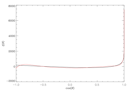
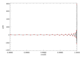
Figure 2: The figure displays the average correlation function in a simulated MAP survey (black) and one realization (red). The inserted panel shows the average noise correlation function (line) with one realization (diamonds).

3 Fast Estimation of the Correlation Function at Legendre Roots

The novel correlation function estimator is based on fast spherical harmonics decomposition; our aim is to make use of their speed, based on the FFT’s of isolatitude pixel annuli. Practical implementation of our estimator is based on the fast transforms available in the HEALPix package. Let us define two unit vectors with angle $\theta$ apart, e.g., $n_{1}=(0,0)$, and $n_{2}=(\theta,0)$ in spherical coordinates. In the continuum limit, the raw weighted pairwise estimator is an average over the rotation group

$$D_{f\delta}(cos\theta)=\frac{1}{8\pi^{2}}\int dgf\delta(R(g)n_{1})f\delta(R(g)n_{2}),$$ (3)

where the integration is over SO(3), $8\pi^{2}$ is the full volume of the Lie group, and R(g) is the transformation corresponding to the Lie group element. The sum in equation (2) is replaced by an integral, multiplicative weighting is assumed: $f_{ij}=f_{i}f_{j}$, and $f\delta\simeq f_{i}\Delta_{i}$ (both taken at the same vector), corresponds to the weighted temperature fluctuations in the continuum limit. After a simple calculation based on the general orthogonality of group representations

$$D_{f\delta}(cos\theta)=\sum_{lm}\mid{a_{lm}}\mid^{2}\frac{1}{4\pi}P_{\ell}(cos\theta),$$ (4)

where the $a_{lm}$’s are the coefficients of the spherical harmonics decomposition of $f\delta$. The ensemble average of the equation yields $\langle{D_{f\delta}}\rangle=(\xi\ +N)D_{f}$, where we introduced the weight correlation function $D_{f}$, calculated similarly to $D_{f\delta}$. The unbiased correlation function estimator can be obtained as

$$\tilde{\xi}(cos\theta)=\frac{D_{f\delta}(cos\theta)-\bar{D}_{fn}(cos\theta)}{D_{f}(cos\theta)},$$ (5)

where $\bar{D}_{fn}$ is the average raw noise correlation function calculated from $M$ simulations; obviously $\langle{\tilde{\xi}}\rangle=\xi$. According to equation (4) this estimator is calculated via two spherical harmonics transforms in discrete pixel space, with the summation performed up to $\ell_{max}$. This is a fast realization of the estimator in equation (2) with multiplicative weights.

We cross-compared the above algorithm with a naive $N^{2}$ correlation code, and the results were identical. To obtain the angular power spectrum, we then sample the above equation exactly at the roots of Legendre polynomials, and perform Gauss-Legendre integration, as done by SPPSB.

The expected scaling is $N^{3/2}{\rm log}N$, corresponding to an effective $N^{1.61}$ slope for the present implementation in the range of $N$ we tested. The speed between calculating the correlation estimator and the $C_{l}$ inversion is divided approximately evenly; on a 500Mhz Dec alpha our present HEALpix compatible implementation takes $\sim$260 seconds, Planck analysis is feasible in about 40 minutes.

The above procedure appears unnatural at first: if we are using FFT’s, and our final goal is to estimate the angular power spectrum, why do we leave Fourier space at all? The reason is simple: window and noise are localized in pixel space, thus we can construct an unbiased estimator with a simple normalization. Such a normalization in pixel space is equivalent to an edge effect correction, and heuristic weights can be constructed intuitively and naturally. In principle an analogous procedure can be designed in $\ell$ space, but the non-diagonality of the window function results in a complex coupling matrix infused with Wigner $3j$ symbols, as Hivon et al. (2001) have shown in a tour de force calculation. The computation and inversion of this matrix to unbias the estimator is highly non-trivial numerically, especially in the presence of noise and complex geometry; so far they have demonstrated numerical feasibility for a relatively simple ellipsoidal window without any noise weighting. It is not inconceivable that this procedure can be successfully extended to more general windows and noise weighting, but at a price which can be regarded as unnecessary complexity; therefore we recommend the simple technique of constructing an unbiased weighted pixel space estimator instead.

4 Application: MAP Simulations

We have generated 1200 MAP simulations using HEALPix with inhomogenous sinusoidal coverage assuming a detector sensitivity of $20\mu K$ for a $0.3^{\circ}\times 0.3^{\circ}$ pixel, taken from the MAP homepage, (http://map.gsfc.nasa.gov/). We assumed a Gaussian beam of $18$ arcminutes, we neglected any sidelobes or asymmetries. Our simulations are similar, although not perfectly equivalent to that of OSH. In addition to the noisy MAP simulations, we have generated 1200 pure noise simulations to be used in our estimator of Equation (2). Our noise weighting was inversely proportional to the expected noise in a pixel, $f_{ij}\simeq 1/(\sigma^{p}_{n_{i}}\sigma^{p}_{n_{j}})$, with $p=1$ motivated by prewhitening, and $p=2$ by approximate minimum variance estimator. Both performed quite similarly, we show the results from $p=2$. We used a galactic cut of $\pm 20$ degrees.

The noise correlations were calculated with the code and were subtracted from the correlation function according to equation (2). While the noise was assumed to be diagonal, our practical implementation does not make use of this property, except in the heuristic noise weighting we adopted. If this assumption would break, our method would not be affected, as long as the simulations can be generated quickly.

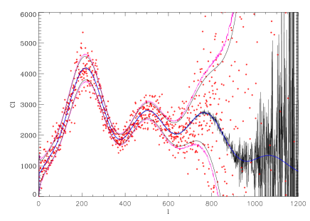
Figure 3: $C_{\ell}$ measurements in MAP simulations are illustrated. The blue line is the underlying theory, while the overlapping black solid line corresponds the the average of 1200 measurements; this explicitly demonstrates the unbiased nature of our technique. The pair of black lines opening up for high $\ell$ displays approximate theoretical error bars, according to equation (6). The magenta lines are error bars calculated from 1200 simulations. They track the theoretical error bars quite well.

The $C_{\ell}$ integration was performed via a Gauss-Legendre quadrature. Beam and pixel window functions were accounted for as usual. The results are displayed in Figure 3. Along with the average $C_{\ell}$, the theoretical input, as well as theoretical and measured errors are displayed, the former from the following approximation (Hivon et al. 2001)

$$\Delta{\cal C}_{\ell}=\sqrt{\frac{2}{\nu_{l}}}\left({\cal C}_{\ell}+B(\ell)^{2}W(\ell)^{2}N(l)\right),$$ (6)

where $\nu_{l}=(2\ell+1)f_{sky}w_{2}^{2}/w_{4}$ with $w_{m}=\frac{1}{4\pi}\int d\Omega f^{m}(\Omega)$, the $m$-th moments of the weight function $f_{i}$, $B(\ell),W(\ell),N(\ell)$ represent beam, pixel, and noise effects, respectively, and $f_{sky}$ is the sky fraction in the map. According to Figure 3 our method is unbiased, and accurate for MAP: the error bars track closely the theoretical expectation within the accuracy of the approximate theory. The suboptimality of our technique is expected to be small for MAP-like surveys, but this needs to be confirmed by detailed comparison to optimal techniques. Our figure is similar to Figure 4 of Oh et al. (1999), but there are small differences: it appears that we have assumed a slightly higher noise and/or wider beam. It would be worthwhile to perform direct comparison of the two methods to assess the degree of suboptimality of ours, and the sensitivity of the experiment specific technique to a potential breakdown of the underlying assumptions.

5 Summary and Discussions

We have demonstrated that i) correlation functions with generalized edge correction can be extracted with full accuracy for a megapixel map in minutes on a modest personal workstation ii) the resulting $C_{\ell}$ computed from Monte-Carlo realizations of MAP observations with inhomogeneous coverage agree quite well with the (approximate) theoretical error bars inferred from the moments of the window function applied to the data to construct our estimator, as well as the cosmic variance. The results should be very close to optimal at high $\ell$ where the noise variance become dominant provided that the noise matrix is diagonally dominant, but this needs to be confirmed by a detailed comparison with optimal methods. The theoretical scaling of our method is $N^{3/2}{\rm log}N$, with a measured scaling of $\sim N^{1.61}$ in our present implementation, for the range of $N$ we tested.

In the previous tests we have used MAP-like diagonal noise/coverage, no other (e.g., azimuthal) symmetries were assumed about noise, or geometry of the map. Cut out holes around bright sources, or any irregularity in the sampling, represent only minor perturbations to our method, therefore they should have no discernible effect on its speed or performance; the investigation of this point in sufficient detail is left for future work. Our approach is straightforward to generalize for non-diagonal noise matrix, specially in the case where the off-diagonal elements of the noise matrix correspond primarily to pairs of pixels of fixed angular separation, as is expected for MAP due to the differential nature of the measurement. In the general case, our main assumption is the fast generation of noise realizations in pixel space, which will be supplied by fast mapmaking methods (e.g. Wright 1996; Prunet et al. 2001).

At the heart of our method is the use of heuristic weighting corresponding to general edge effect correction. (Indeed, noise can be considered as a fuzzy window, or window can be considered as infinite noise). The simplicity of our weighting amounts to a substantial gain in speed over the costly optimal weighting $(S+N)^{-2}$. In addition, the use of spherical harmonics decomposition facilitates heuristic signal weighting, which is natural in $\ell$ domain. The sum of the $a_{lm}$’s in equation (4) can be recognized as a pseudo $C_{l}$ of the weighted fluctuations estimated with uniform weights in $\ell$ space. For low $\ell$’s, for complicated noise and window patterns, it might be desirable to sum the $a_{lm}$’s with weights obtained from the correlation matrix $<a_{l_{1}m_{1}}a_{l_{2}m_{2}}>$ evaluated from Monte Carlo simulations. This matrix can be diagonalized e.g. up to a certain $\ell$, or within a band of $\Delta\ell$, to calculate approximate (semi-heuristic) weights for our estimator of the correlation function. While such improvements do not seem necessary for MAP, a clear upgrade path for our method exists for more complex experiments if needed. Although more natural in $\ell$ space, heuristic signal weighting is possible in pixel space as well (e.g., Colombi, Szapudi, & Szalay 1998).

Our technique has further potential besides speeding up $C_{l}$ estimation: it opens up a full array of possible applications and generalizations. These include cross-correlations (between channels for component separation, between LSS and CMB, B-type polarization and lensing, etc) non-Gaussianity (e.g. 3-point function/bispectrum, cumulant correlators for SZ, lensing, etc), vector and tensor correlations (for polarization). The idea of real space window and noise weighting is applicable to power spectrum estimators of galaxies, clusters, lensing etc. as well. A Euclidian version of our algorithm is entirely analogous to the spherical case. It will be useful for fast edge and noise corrected estimation of the power spectrum, bispectrum, $N$-point correlation function and cumulant correlators in galaxy catalogs. These generalizations presently under implementation will be discussed in subsequent papers and included in a later version of SpICE.

We would like to thank Dick Bond, Dmitry Pogosyan, Alex Szalay for their help, and Carlo Contaldi and Eric Hivon for useful discussions. This research was supported by NASA through the Applied Information Systems Research program (NAG5-10750).

References

- (1) Bond J.R., 1995, Phys. Rev. Lett., 74, 4369
- (2) Bond, J.R., Efstathiou, G., & Tegmark, M. 1997, MNRAS, 291, L33
- (3) Bond, J.R., Jaffe, A.H. & Knox, L. 1998, Phys. Rev. D, 57, 2117
- (4) Bond, J.R., Jaffe, A.H. & Knox, L. 2000, ApJ, in press
- (5) Borrill, J., 1999, Proc. of the 5th European SGI/Cray MPP
- (6) Bunn, E.F, & White, M. 1997, ApJ, 480, 6
- (7) Colombi S., Szapudi I., Szalay A.S., 1998, MNRAS, 296, 253
- (8) de Bernardis, et al. 2000, Nature, 404, 955
- (9) Górski, K.M. 1994, ApJ, 430, L85
- (10) Górski, K.M et al. & 1994, ApJ, 430, L89
- (11) Górski, K.M et al. & 1996, ApJ, 464, L11
- (12) Hanany, S. et al. , 2000, ApJ, submitted (astro-ph/0005123)
- (13) Hinshaw, G., Bennett, C.L., & Kogut, A. 1995, ApJ, 441, L1
- (14) Hivon, E., et al. 2001, ApJ, submitted (astro-ph/01055302)
- (15) Jaffe, A.H., etal, 2001, Phys. Rev. Lett.86, 3475
- (16) Jungman, G., Kaminonkowski, M., Kosowski, A., & Spergel, D.N. 1996, Phys. Rev. D, 54, 1332
- (17) Knox, L. 1995, Phys. Rev. D, 52, 4307
- (18) Martin, N., et al. 1996, in Space Telescopes and Instruments IV Proc. SPIE (eds. P. Y. Bely and J. B. Breckinridge), 2807, 86
- (19) Miller, A.D., et al. 1999, ApJ, 524, 1
- (20) Netterfield, C.B. et al. 2001, ApJ, submitted (astro-ph/0104460)
- (21) Oh, S.P., Spergel, D.N., & Hinshaw, G. 1999, ApJ, 510, 551
- (22) Peterson, J.B., et al. 2000, ApJ, 532, 83
- (23) Prunet, S., et al. 2001, astro-ph/0101073
- (24) Tegmark, M. 1996, ApJ, 464, L35
- (25) Tegmark, M. & Bunn, E.F. 1995, ApJ, 455, 1
- (26) Smoot et al. 1992, ApJ, 396, L1
- (27) Spergel, D.N. 1994, Warner Prize Lecture, BAAS, 185.7301
- Szapudi & Szalay (1998) Szapudi, I. & Szalay, A.S. 1998, ApJ, 494, L41 (SS)
- (29) Szapudi, I., Prunet, S., Pogosyan, D., Szalay, A.S., & Bond, J.R. 2001, ApJ, 548, L11 (SPPSB)
- (30) Zaldarriaga, M., Spergel, D.N., & Seljak, U. 1997, ApJ, 488, 1
- (31) Wandelt, B. D, 2000, astro-ph/0012416
- (32) Wright, E.L., 1996 (astro-ph/9612105)
- (33) Wright, E.L., Hinshaw, G. & Bennett, C.L. 1996, ApJ, 458, L53