Are some breaks in GRB afterglows caused by their spectra?

Sharp breaks have been observed in the afterglow light curves of several GRBs; this is generally explained by the jet model. However, there are still some uncertainties concerning this interpretation due to the unclear hydrodynamics of jet sideways expansion. Here we propose an alternative explanation to these observed breaks. If we assume that the multiwavelength spectra of GRB afterglows are not made of exact power law segments but their slope changes smoothly, i.e. $d\beta/dlog\nu<0$, where $\beta$ is the spectral index, we find that this fact can very nicely explain the afterglow light curves showing breaks. Therefore we suggest that some breaks in the afterglow light curves may be caused by their curved spectra. The main feature of this interpretation is that the break time is dependent on the observed frequency, while the jet model produces achromatic breaks in the light curves. In addition, it is very important to know the position of the characteristic frequency $\nu_{c}$ in the multiwavelength spectrum at the time of the break, since it is a further discriminant between our model and the jet model. We find that although the optical light curves of seven GRB afterglows can be well fitted by the model we propose, in fact only one of them (i.e. GRB000926) can be explained in this framework, since for other ones the characteristic frequency $\nu_{c}$ is either above the optical after the break or below the optical before the break.

1 Introduction

It is widely accepted that the emission from GRB afterglows can be well described by the fireball model, in which the ejecta from an underlying explosion expand into the surrounding medium, producing a relativistic shock(e.g. Piran 1999 and references therein). In the standard picture, the electrons are accelerated to relativistic energies, with their Lorentz factors described by a simple power law distribution $N(\gamma_{\rm e})\propto\gamma_{\rm e}^{-p}$ above the minimum value $\gamma_{\rm m}$. Besides particle acceleration, the shock is also responsible for the creation of a strong magnetic field. Under these conditions the electrons radiate synchrotron emission; thus, the afterglow flux is $f(t,\nu)\propto t^{\alpha}\nu^{\beta}$, where the temporal index ($\alpha$) and the spectral index ($\beta$) are related to $p$ and the dynamics of the blast wave (Wijers et al. 1997; Wei & Lu 1998; Sari et al. 1998; Huang et al. 2000).

The optical light curves of afterglows can generally be described by a single power law decay with index $\alpha\simeq-1.1\sim-2$. However, changes in the light decay rate, with a transition to a steeper power law behavior have been detected in several GRBs(GRB990123: Kulkarni et al. 1999, Castro-Tirado et al. 1999; GRB990510: Harrison et al. 1999, Stanek et al. 1999; GRB000301C: Rhoads & Fruchter 2001, Masetti et al. 2000b; GRB000926: Sagar et al. 2001a, Price et al. 2001, Fynbo et al. 2001; GRB010222: Masetti et al. 2001, Stanek et al. 2001, Cowsik et al. 2001, Sagar et al. 2001b; GRB991216: Halpern et al. 2000, Sager et al. 2000; GRB991208: Castro-Tirado et al. 2001; GRB990705: Masetti et al. 2000a). Such breaks are usually explained by the jet model. Rhoads (1997; 1999) and Sari et al. (1999) have pointed out that the lateral expansion of the relativistic jet will cause a change in the hydrodynamic behavior and hence a break in the light curve. However, jet evolution and emission are very complicated processes, for which different analytic or semi-analytic calculations lead to different predictions for the sharpness of the jet break, the jet break time and the duration of the transition. For example, Rhoads (1999) claimed that jet expansion produces sharp breaks in the light curves, while some numerical calculations show that breaks occur smoothly and gradually (Panaitescu & Meszaros 1999; Moderski et al. 2000; Kumar & Panaitescu 2000; Wei & Lu 2000a,b). In particular, the light curve of GRB010222 seems difficult to be explained by the jet model (Masetti et al. 2001; Dai & Cheng 2001).

Here we propose an alternative explanation for these observed breaks. We assume that the multiwavelength spectra of GRB afterglows are not made of exact power law segments, but that their slope changes smoothly, i.e. $d\beta/dlog\nu<0$. We find that this model can nicely explain at least one of the afterglow light curves showing breaks. In next section we describe our model and show the effect of the curved spectra on the afterglow light curves; after this, some discussions and conclusions are given.

2 The effect of curved spectra on afterglow light curve

In the fireball model the afterglow emission spectrum is described by Sari et al. (1998) as a series of 4 different power law segments, continuously connecting in correspondence of 3 characteristic synchrotron frequencies ($\nu_{\rm a}$, $\nu_{\rm m}$ and $\nu_{\rm c}$). However, it is likely that these connections are not as sharp as in the modelization of Sari et al. (1998); indeed, in some cases a smooth reconnection over the synchrotron characteristic frequencies listed above has been hypothesized (e.g. Granot & Sari 2001). Therefore, a smooth spectral bending over $\nu_{\rm a}$, $\nu_{\rm m}$ and $\nu_{\rm c}$, which implies a curved spectrum, can be considered as a reasonable assumption. In this hypothesis, the slope of the spectra changes as $d\beta/dlog\nu<0$, where the spectral index $\beta$ is defined as $\beta=dlogF_{\rm\nu}/d\log\nu$.

Now let us consider the standard case, i.e. the one in which the blast wave is isotropic and adiabatic, the surrounding medium is homogeneous, and the afterglow emission is mainly produced by synchrotron radiation from accelerated electrons. Under these conditions, Sari et al. (1998) have computed the characteristic synchrotron frequencies

$$\nu_{\rm m}=5.7\times 10^{11}(\frac{\epsilon_{\rm B}}{10^{-2}})^{1/2}(\frac{\epsilon_{\rm e}}{0.1})^{2}E_{52}^{1/2}t_{\rm d}^{-3/2}\;\;\;\;{\rm Hz}$$ (1)

$$\nu_{\rm c}=2.7\times 10^{15}(\frac{\epsilon_{\rm B}}{10^{-2}})^{-3/2}E_{52}^{-1/2}n_{1}^{-1}t_{\rm d}^{-1/2}\;\;\;\;{\rm Hz}$$ (2)

where $\nu_{\rm m}$ is the emission frequency corresponding to the minimum electron Lorentz factor $\gamma_{\rm m}$, $\nu_{\rm c}$ is the cooling frequency, $E_{52}$ is the fireball energy in units of $10^{52}\,erg$, $\epsilon_{\rm e}$ and $\epsilon_{\rm B}$ are the energy fractions of electrons and magnetic field respectively, $n_{1}$ is the surrounding medium density in units of $1\,\,{\bf atom}\,\,{\rm cm^{-3}}$, and $t_{\rm d}$ is the time since burst in units of $1\,{\rm day}$. It is obvious that, for typical parameters, $\nu_{\rm m}$ is usually far below the optical band few hours after the GRB, while $\nu_{\rm c}$ is generally close to the spectral ranges in which breaks are observed (i.e. optical and X-rays), so we assume that the curved spectrum has the form

$$F_{\nu}=2F_{\nu_{\rm c}}[(\frac{\nu}{\nu_{\rm c}})^{\beta_{1}}+(\frac{\nu}{\nu_{\rm c}})^{\beta_{2}}]^{-1}\;\;\;\;for\;\;\;\;\nu>\nu_{\rm m}$$ (3)

where $\beta_{2}>\beta_{1}>0$. Thus for $\nu\ll\nu_{\rm c}$, $F_{\nu}\propto\nu^{-\beta_{1}}$, and for $\nu\gg\nu_{\rm c}$, $F_{\nu}\propto\nu^{-\beta_{2}}$. Since for typical parameters $\nu_{\rm m}\ll\nu_{\rm c}$, we have $F_{\nu_{\rm m}}=2F_{\nu_{\rm c}}(\frac{\nu_{\rm m}}{\nu_{\rm c}})^{-\beta_{1}}$. In the standard case, the evolution of the bulk Lorentz factor is $\Gamma\propto t^{-3/8}$, the peak flux $F_{\nu_{\rm m}}\propto t^{0}$, and $\nu_{\rm m}/\nu_{\rm c}\propto t^{-1}$ (e.g. Piran 1999 and references therein), so we have $F_{\nu_{\rm c}}\propto t^{-\beta_{1}}$. Then, for a fixed frequency $\nu_{\rm obs}$, the afterglow light curve is

$$F_{\nu_{\rm obs}}\propto\frac{(\frac{t}{t_{\rm c}})^{-\frac{3}{2}\beta_{1}}}{1+(\frac{t}{t_{\rm c}})^{\frac{1}{2}(\beta_{2}-\beta_{1})}}\;\;\;for\;\;t>t_{\rm m}$$ (4)

where $t_{\rm m}$ and $t_{\rm c}$ are the time when $\nu_{\rm m}$ and $\nu_{\rm c}$ cross the fixed frequency $\nu_{\rm obs}$. So we have $F_{\nu_{\rm obs}}\propto t^{-\frac{3}{2}\beta_{1}}$ for $t\ll t_{\rm c}$, and $F_{\nu_{\rm obs}}\propto t^{-(\beta_{1}+\frac{1}{2}\beta_{2})}$ for $t\gg t_{\rm c}$.

The main feature of this interpretation is that the break time is dependent on the observed frequency, i.e. the break time is larger for smaller frequencies. In the present model, the break occurs when the characteristic frequency $\nu_{\rm c}$ crosses the observed frequency $\nu_{\rm obs}$. Since $\nu_{\rm c}\propto t^{-1/2}$ in the standard case, the break time $t_{\rm b}\propto\nu_{\rm obs}^{-2}$. Therefore the ratio of the break time of X-ray and optical is $t_{\rm bX}/t_{\rm bo}=(\nu_{\rm X}/\nu_{\rm o})^{-2}\approx 10^{-6}$. On the contrary, for the jet model (Rhoads 1999; Sari et al. 1999) or the transition from a relativistic to a non-relativistic regime (Dai & Lu 1999) the break time is achromatic, so it is easy to distinguish between these breaks and the one produced by a smoothly curved spectrum. In addition, it is very important to know the position of the characteristic frequency $\nu_{\rm c}$ in the multiwavelength spectrum at the time of the break, since it is a further discriminant between our model and the jet model.

Based on the above results, we have fitted the optical light curves of seven GRB afterglows in which breaks were detected. In Figs.1 to 7 we see that this model can fit some of the observed data very well. However, from Fig.3 we see that deviations of the GRB000301C light curve from the fit are evident; this is due to the existence of flux fluctuations in the optical light curve. These short time scale variations can be explained by, for instance, microlensing (Garnavich et al. 2000), or by the re-energization of the blast wave, or by irregularities of the interstellar medium (see e.g. Masetti et al. 2000b). Thus, these deviations are not connected with either the jet model or with ours. If we ignore these fluctuations, the overall fit appears more satisfactory, with a reduced $\chi^{2}=1.8$. In addition, the reduced $\chi^{2}$ value of GRB010222 is high, which is due to the possible existence of a further break about 20 days after the burst, and also due to the microvariability in the observed optical data, so is not connected with our model.

Besides optical light curves, X-ray light curves are also available for four GRB afterglows (GRB990510: Pian et al. 2000; GRB000926: Piro et al. 2001; GRB010222: in’t Zand et al. 2001; GRB991216: Halpern et al. 2000), and it is important to compare our model with these light curves to see whether it could fit the decays in different energy ranges, keeping in mind that this model foresees an energy-dependent break. We have fitted the observed X-ray data using the parameters which best fit the optical light curves (for the X-ray break time, we adopt $t_{\rm cx}=t_{\rm c}(\nu_{\rm X}/\nu_{\rm o})^{-2}\simeq 10^{-6}t_{\rm c}$), and in Figs.4-6 we see that our model can fit also the X-ray light curves of GRB010222, GRB000926 and GRB991216 quite well (although the reduced $\chi^{2}$ value of GRB000926 is somewhat high this is due to the last data point which seems to indicate a second break in the light curve (see Piro et al. 2001). If we ignore the last point, then the reduced $\chi^{2}$ value of the fit is 0.93). It is instead obvious (see Fig.2) that the X-ray light curve of GRB990510 cannot be fitted by our model.

However, we note that, for GRB990123 (Castro-Tirado et al. 1999), GRB010222 (Masetti et al. 2001), GRB991216 (Halpern et al. 2000), and GRB990510 (Pian et al. 2001), $\nu_{\rm c}$ lies well above the optical window after the light curve break, while for GRB000301C (Jensen et al. 2001) the frequency $\nu_{\rm c}$ is below the optical range before the light curve break, so these GRBs cannot be explained by this model. Only for GRB000926 (Harrison et al. 2001) $\nu_{\rm c}$ is located below the optical range after the light curve break, thus this break can be explained by our model.

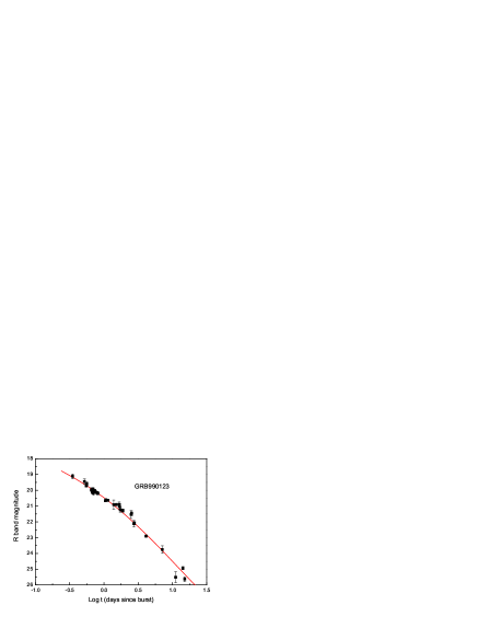
Figure 1: The R-band light curve of the GRB990123 afterglow; the contribution of host galaxy has been subtracted. The solid line represents our best fit assuming the model described in the text. The fit parameters are: $\beta_{1}=0.52$, $\beta_{2}=2.8$, $t_{\rm c}=1.2\,{\rm days}$, the reduced $\chi^{2}=2.1$.

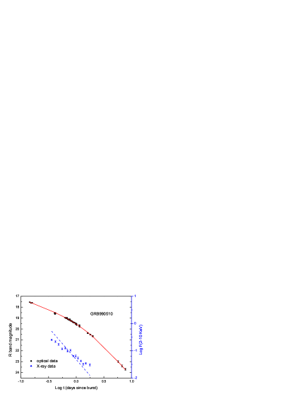
Figure 2: The R-band and X-ray light curves of the GRB990510 afterglow. The solid line represents our best fit to the optical data assuming the model described in the text. The fit parameters are: $\beta_{1}=0.49$, $\beta_{2}=3.7$, $t_{\rm c}=1.4\,{\rm days}$, the reduced $\chi^{2}=2.13$. The dashed line represents the fit to the X-ray data using the above parameters, the value of reduced $\chi^{2}$ for X-ray fitting is 33.

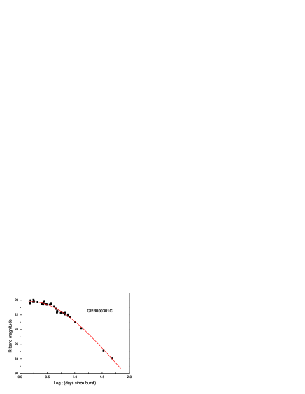
Figure 3: The R-band light curve of the GRB000301C afterglow. The solid line represents our best fit assuming the model described in the text. The fit parameters are: $\beta_{1}=0.2$, $\beta_{2}=5.6$, $t_{\rm c}=4.9\,{\rm days}$, the reduced $\chi^{2}=5.8$.

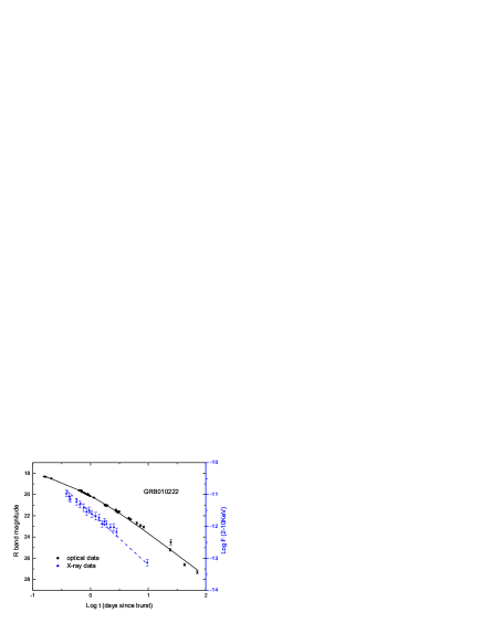
Figure 4: The R-band and X-ray light curves of the GRB010222 afterglow. The solid line represents our best fit to the optical data assuming the model described in the text. The fit parameters are: $\beta_{1}=0.4$, $\beta_{2}=2.5$, $t_{\rm c}=0.9\,{\rm days}$, the reduced $\chi^{2}=6.1$. The dashed line represents the fit to the X-ray data using the above parameters, the value of reduced $\chi^{2}$ for X-ray fitting is 0.86.

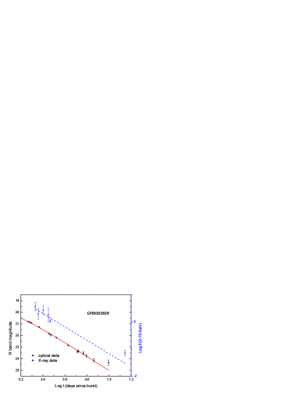
Figure 5: The R-band and X-ray light curves of the GRB000926 afterglow. The solid line represents our best fit to the optical data assuming the model described in the text. The fit parameters are: $\beta_{1}=0.37$, $\beta_{2}=4.2$, $t_{\rm c}=1.0\,{\rm days}$, the reduced $\chi^{2}=1.49$. The dashed line represents the fit to the X-ray data using the above parameters, the value of reduced $\chi^{2}$ for X-ray fitting is 4.1.

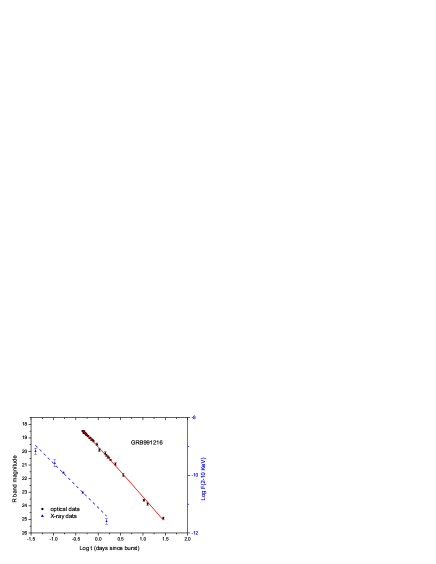
Figure 6: The R-band and X-ray light curves of the GRB991216 afterglow. The solid line represents our best fit to the optical data assuming the model described in the text. The fit parameters are: $\beta_{1}=0.54$, $\beta_{2}=2.0$, $t_{\rm c}=0.11\,{\rm days}$, the reduced $\chi^{2}=0.94$. The dashed line represents the fit to the X-ray data using the above parameters, the value of reduced $\chi^{2}$ for X-ray fitting is 2.

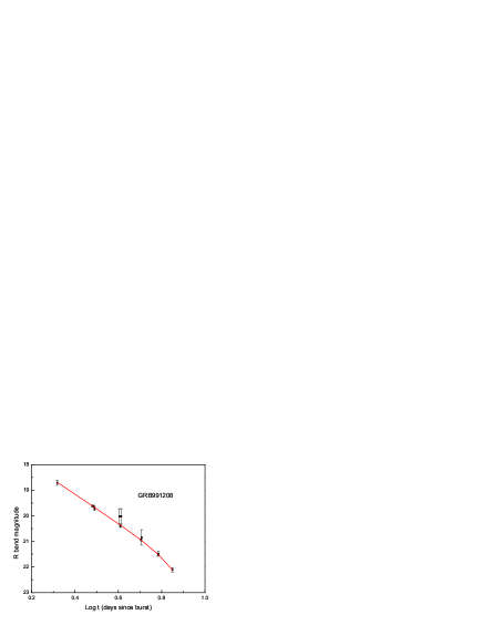
Figure 7: The R-band light curve of the GRB991208 afterglow. The solid line represents our best fit assuming the model described in the text. The fit parameters are: $\beta_{1}=1.5$, $\beta_{2}=14.6$, $t_{\rm c}=8\,{\rm days}$, the reduced $\chi^{2}=0.5$.

3 Discussion and conclusions

In this paper we assumed that GRB afterglow spectra are not made of simple power law segments, but the spectral index changes gradually with frequency across the afterglow characteristic synchrotron frequencies. Under these conditions, we have shown that, even in the standard afterglow model, the afterglow optical light curves showing breaks can be fitted very well and, except for GRB990510, the afterglow X-ray light curves can also be fitted quite well. So we propose that the effects of the curved spectra on the light curves should not be ignored.

For the simple spectral form we adopted here (Eq.3), considering a fixed frequency $\nu_{\rm obs}$, the spectral index $\beta$ is assumed to change with time, so it is of paramount importance to accurately monitor the GRB afterglow spectral evolution to test the hypotheses behind the model presented here. In addition, it is also necessary to improve the energy and time resolution of the observations in order to verify the presence of a small curvature of the spectra.

Here we simply take the curved spectra in the form of Eq.(3), but several physical mechanisms may be responsible for this. The curved spectra may be caused by intrinsic or intervening absorption, or by steepening of the electron energy distribution, or by smooth connection of the power-law segments over the characteristic synchrotron frequencies.

In summary, here we have shown that the curved spectra can produce sharp breaks in the afterglow light curves; however, not all breaks can be explained by this effect. We think that some of the steepenings observed in the afterglow light curves may be the combined result of a curved spectrum and of a collimated fireball. Future observations will test this hypothesis.

- (1) Castro-Tirado, A.J., Zapatero-Osorio, M.R., Caon, N., et al., 1999, Science, 283, 2069
- (2) Castro-Tirado, A.J., Sokolov, V.V., Gorosabel, J., et al., 2001, A&A, 370, 398
- (3) Cowsik, R., Prabhu, T.P., Anupama, G.C., et al., 2001, Bull. Astron. Soc. India, in press(astro-ph/0104363)
- (4) Dai, Z.G., Lu, T., 1999, ApJ, 519, L155
- (5) Dai,Z.G., Cheng, K.S., 2001, ApJ, 558, L109
- (6) Fynbo, J.U., Gorosabel, J., Dall, T.H., et al., 2001, A&A, 373, 796
- (7) Garnavich, P., Loeb, A., Stanek, K.Z., 2000, ApJ, 544, L11
- (8) Granot, J., Sari, R., 2001, ApJ, submitted (astro-ph/0108027)
- (9) Halpern, J.P., Uglesich, R., Mirabal, N., et al., 2000, ApJ, 543, 697
- (10) Harrison, F.A., Bloom, J.S., Frail, D.A., et al., 1999, ApJ, 523, 121
- (11) Huang, Y.F., Gou, L.J., Dai, Z.G., Lu, T., 2000, ApJ, 543, 90
- (12) In’t Zand, J.J.M., Kuiper, L., Amati, L., et al., 2001, ApJ, 559, 710
- (13) Jensen, B.L., Fynbo, J.U., Gorosabel, J., et al., 2001, A&A, 370, 909
- (14) Kulkarni, S.R., Djorgovski, S.G., Odewahn, S.C., et al., 1999, Nature, 398, 389
- (15) Kumar, P., Panatescu, A., 2000, ApJ, 541, L9
- (16) Masetti, N., Palazzi, E., Pian, E., et al., 2000a, A&A, 354, 473
- (17) Masetti, N., Bartolini, C., Bernabei, S., et al., 2000b, A&A, 359, L23
- (18) Masetti, N., Palazzi, E., Pian, E., et al., 2001, A&A, 374, 382
- (19) Moderski, R., Sikora, M., Bulik, T., 2000, ApJ, 529, 151
- (20) Panaitescu, A., Mészáros, P., 1999, ApJ, 526, 707
- (21) Pian, E., Soffitta, P., Alessi, A., et al., 2001, A&A, 372, 456
- (22) Piran, T., 1999, Phys. Rep., 314, 575
- (23) Piro, L. Garmire, G., Garcia, M.R., , et al., 2001, ApJ, 558, 442
- (24) Price, P.A., Harrison, F.A., Galama, T.J., et al., 2001, ApJ, 549, L7
- (25) Rhoads, J.E., 1997, ApJ, 487, L1
- (26) Rhoads,J.E., 1999, ApJ, 525, 737
- (27) Rhoads,J.E., Fruchter, A.S., 2001, ApJ, 546, 117
- (28) Sagar, R., Mohan, V., Pandey, A.K., Pandey, S.B., Castro-Tirado, A.J., 2000, Bull. Astron. Soc. India, 28, 15 (astro-ph/0003257)
- (29) Sagar, R., Pandey, S.B., Mohan, V., Bhattacharya, D., Castro-Tirado, A.J., 2001a, Bull. Astron. Soc. India, 29, 1 (astro-ph/0010212)
- (30) Sagar, R., Stalin, C.S., Bhattacharya, D., et al., 2001b, Bull. Astron. Soc. India, 29, 91(astro-ph/0104249)
- (31) Sari, R., Piran, T., Narayan, R., 1998, ApJ, 497, L17
- (32) Sari, R., Piran, T., Halpern, J.P., 1999, ApJ, 519, L17
- (33) Stanek, K.Z., Garnavich, P.M., Kaluzny, J., Pych, W., Thompson, I., 1999, ApJ, 522, L39
- (34) Stanek, K.Z., Garnavich, P.M., Jha, S., et al., 2001, ApJ, in press (astro-ph/0104329)
- (35) Wei, D.M., Lu, T., 1998, ApJ, 499, 754
- (36) Wei, D.M., Lu, T., 2000a, ApJ, 541, 203
- (37) Wei, D.M., Lu, T., 2000b, MNRAS submitted (astro-ph/0012007)
- (38) Wijers, R.A.M.J., Rees, M.J., Mészáros, P., 1997, MNRAS, 288, L51