The Evolution of Adiabatic Supernova Remnants in a Turbulent, Magnetized Medium

Abstract

We present the results of three dimensional calculations for the MHD evolution of an adiabatic supernova remnant in both a uniform and turbulent interstellar medium using the RIEMANN framework of Balsara. In the uniform case, which contains an initially uniform magnetic field, the density structure of the shell remains largely spherical, while the magnetic pressure and synchrotron emissivity are enhanced along the plane perpendicular to the field direction. This produces a bilateral or barrel-type morphology in synchrotron emission for certain viewing angles. We then consider a case with a turbulent external medium as in Balsara & Pouquet, characterized by $v_{A}(rms)/c_{s}=2$. Several important changes are found. First, despite the presence of a uniform field, the overall synchrotron emissivity becomes approximately spherically symmetric, on the whole, but is extremely patchy and time-variable, with flickering on the order of a few computational time steps. This is reminiscent of the Cas A observations of Anderson & Rudnick, although that remnant has a much more complicated pre-supernova evolution than what is considered here. We suggest that the time and spatial variability of emission in early phase SNR evolution provides information on the turbulent medium surrounding the remnant. The interaction of the outwardly-propagating SNR shock with interstellar turbulence is shown to amplify the turbulence in the post-shock region, thereby having important consequences for relativistic particle acceleration. The shock-turbulence interaction is also shown to be a strong source of helicity-generation and, therefore, has important consequences for magnetic field generation. We compare our calculations to the Sedov-phase evolution, and discuss how the emission characteristics of SNR may provide a diagnostic on the nature of turbulence in the pre-supernova environment.

1 Introduction

The morphology and emission of supernova remnants (SNRs) is in large part determined by the nature of the surrounding circumstellar and interstellar medium. Young SNRs from massive stars interact with a significant mass of former wind material expelled by the star, sometimes knotty and irregular, sometimes with significant preshaping by the complex wind history. Older SNRs in the halo of the Galaxy will have low X-ray surface brightness (Shelton et al 1998). SNRs in dense molecular clouds will eventually be elongated in the direction of the density gradient (Cox et al 1999). SNRs at the edges of clouds will develop offsets between the morphological and kinematic centers (Dohm-Palmer et al 1996). Barrel-shaped remnants may probe the global magnetic field structure (Gaensler 1998), and so on.

There have been several calls by observers, see Dickel, van Breugel & Strom (1991), Reynolds & Gilmore (1993), Reed et al (1995) and others, to introduce a realistic representation of interstellar turbulence in SNR simulations. This need has been mirrored in the work of theorists, see for example Jun & Jones (1999), who claim that without the inclusion of turbulence several observed effects are difficult to match. In particular, Jun & Jones (1999) find their simulated synchrotron indices to be too smooth and uniform and not in line with the patchy observations of Anderson & Rudnick (1996). The problem of including MHD turbulence in such simulations is daunting because of the high demands on resolution and dynamic range. It is now feasible to do these simulations.

We have carried out the first 3D MHD simulations of a supernova going off in a turbulent, magnetized ISM. For comparison we have also carried out a simulation of an identical SNR going off in a uniform but magnetized, non-turbulent ISM. The model includes no pre-supernova wind, no radiative cooling, no thermal conduction and no activity of a central pulsar. It is thus most relevant to the history of Type 1a remnants prior to shell formation, exclusive of the characteristics of the hot interior which would be altered by thermal conduction. More significantly, however, it enlarges our intuition with regard to analytic models, giving us some new insights into the significant effects that interaction with turbulence can have.

2 The Calculations

The simulations presented here are calculated using the RIEMANN framework for parallel, self-adaptive computational astrophysics described in Roe & Balsara (1996), Balsara (1998a,b), Balsara (1999a,b,c,d,e), Balsara & Spicer (1999a,b), Balsara & Shu (2000), Balsara (2001a,b) and Balsara & Norton (2001). This framework uses some of the most accurate higher order Godunov methods for non-relativistic and relativistic MHD and radiative transfer that have been devised. The advantages of this method, particularly in modeling turbulent flows, is described in the above references. The RIEMANN framework has been applied and tested on numerous computational astrophysics problems that require numerical 3D-MHD. It has been used to study the inverse cascade of magnetic helicity (Balsara & Pouquet 1999), star formation studies including the effects of turbulence (Balsara, Crutcher & Pouquet 2001; Balsara, Ward-Thompson & Crutcher 2001), numerical MHD dynamos (Balsara 2000), and AMR-MHD simulations of SNRs and shock-cloud interaction (Balsara 2001c).

We present the results of two high-resolution runs, $(256)^{3}$ zones, comparing the results of evolution in a medium with a uniform and turbulent medium. In both calculations, the physical length of the computational domain is $L=60$ pc. The results presented here were obtained using a uniform mesh and do not utilize the adaptive mesh capability of RIEMANN. In the case of the uniform medium, the initial hydrogen particle density is $1~{}{\rm cm^{-3}}$; the initial temperature is 8000 K ($c_{s}=9.8~{}{\rm km~{}s^{-1}}$), the initial velocities are zero and there is a uniform magnetic field with strength $3.57\mu G$ parallel to the x-axis. The energy input of the supernova is introduced by increasing the thermal energy of all the zones within 2 pc of the center of the computation grid so that the total thermal energy integrated over a spherical volume is $10^{51}$ ergs. The particle density in this volume is also increased to $4~{}{\rm cm^{-3}}$ , corresponding to an ejecta mass of $5~{}M_{\sun}$. The simulations are evolved to the point when the shock reaches the computational boundary. Since there is no cooling or other physical effects that set a physical scale, these parameters may be rescaled without requiring additional simulations.

In the case of the turbulent ISM, the initial conditions are the same as above. The uniform magnetic field is still retained, as described in the previous paragraph. However, we introduce random Gaussian fluctuations in the velocity and magnetic fields, corresponding to $v_{A}(rms)/c_{s}=2$ [$B(rms)=8.94\mu G$] and $v(rms)/c_{s}=2$. (See Balsara & Pouquet 1999 for more details). As a result of the set up we have a uniform mean field as well as a random magnetic field superposed on it. The fluctuating field component is $2.5$ times larger than the uniform field component as a result of the trans-Alfvenic initial conditions. These initial conditions are consistent with the observations of Lee & Jokipii (1976), Beck (1991), and Beck et al. (1996), who find that the Galactic magnetic field has a uniform component as well as a fluctuating component with the two components being in rough equipartition. The Galaxy’s ISM has Mach numbers in the range of one to two and our use of $v_{A}(rms)/c_{s}=2$ would be considered a rather strong turbulence. We made this choice because we seek to study the evolution of supernova remnants in strong interstellar turbulence as a counterpoint to the quiescent medium in the previous simulation. As the blast wave sweeps outward, there is some evolution in the preshock medium, with growing density fluctuations and decaying magnetic and velocity fluctuations. These fluctuations quickly establish an energy power spectrum of $E(k)\propto k^{-5/3}$ in the surrounding medium well before the blast wave propagates a large distance. Thus almost all of the SNR evolution takes place in a fully developed interstellar turbulence. In the present simulations it is not possible to drive the turbulence in order to sustain it at its originally imposed level. This is because such driving mechanisms entail imparting momentum fluctuations to the ISM gas and would, therefore, interfere with the SNR shock propagation. However, the largest energy-bearing length scales have an eddy turnover time of $2.35\times 10^{5}$ years which ensures that there is always sufficient turbulent energy available at the smaller length scales to ensure that the SNR shock interacts with a realistic turbulence during the entire course of the simulation. The rms magnetic field decays less than 15% during our calculated evolution.

3 Results

Despite the presence of a magnetic field, the pressure jump associated with the shock is sufficiently strong that the explosion evolution agrees quite well with the analytical Sedov solution. We find that the position of the shell is given by $R_{Sedov}\propto t^{-2/5}$. The density profile is found to be self-similar and is also in good agreement with the Sedov solution. However, limited resolution prevents us from getting the full factor of four density jump right at the shock front. At early times, the postshock density is 2.6 times greater than the preshock density, increasing with age to 3.3 as more zones are overtaken by the outward-propagating shock wave. The final timestep shown in Figure 1 at $t=57,700$ years, has the following Sedov characteristics, $R=25.5$ pc, $v_{shock}=174~{}{\rm km~{}s^{-1}}$, $T_{2}=4.2\times 10^{5}$ K and $p_{2}=5.2\times 10^{-10}~{}{\rm dynes~{}cm^{-2}}$. The calculated values agree with these analytical estimates. This is just about the oldest this remnant could get without radiative cooling playing a significant role, although with the turbulence there may be some over-dense spots in which cooling might not be negligible. We intend to incorporate this effect in future work.

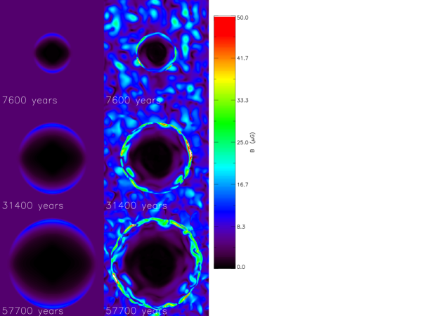
Figure 1: Total magnetic field strength for a two dimensional cut in the XZ plane. Panels on the left show magnetic field strength for the case with a uniform interstellar medium, while the right panel shows the evolution for a turbulent interstellar medium.

The most notable feature of the uniform ISM simulation is that the uniform magnetic field, initially parallel to the x-axis, is swept up into a compressed shell in the XZ plane (See Figure 1). Using an estimated synchrotron emissivity of $pB^{1.5}$ , this produces a bilateral (or barrel-like) morphology for the SNR. Our assumption of a synchrotron emissivity that scales as $pB^{1.5}$ is based on the work of Jun & Jones (1999) who show that it is a natural result of a momentum distribution of accelerated particles with a power law index of 4.

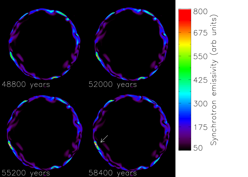
Figure 2: Estimated synchrotron intensity ($\epsilon\propto pB^{1.5}$) for four closely related times. This shows large variablity in intensity for different emission knots. Note, for example the disappearance of bright spot in the lower right side of the remnant and the appearance of bright knots on the upper and lower right sides. This last emission knot is noted with an arrow.

Several differences result for the case of a remnant evolving in a turbulent medium. We have verified that the azimuthally averaged density profile evolves self-similarly and agrees with the Sedov solution. However, in any given radial shell, there are significant azimuthal variations in density just behind the blast wave. The ambient medium is characterized by fluctuations which grow from $\delta\rho/\rho\approx 0.1$ to 0.4 over the course of the simulation. At the shock front, the level of density fluctuations, defined as $\frac{<\delta\rho>}{\rho}_{post-shock}/\frac{<\delta\rho>}{\rho}_{pre-shock}$, jumps by a factor of 4 at early times. At late times, this value declines to $\sim 20$% , presumably because as the surface area of the remnant increases, individual lumps become less important. Behind the shock front, $\delta\rho/\rho$ decreases as the increased thermal pressure works to smooth out the density fluctuations. This behavior is also consistent with one dimensional shock-turbulence interaction studies reported in Balsara & Shu (2000) and has also been observed by several other authors cited in that work.

The variation in the magnetic field is shown in Figure 1 and is especially noteworthy. The overall shape of the remnant is again spherical, but with large azimuthal variations. The mean magnetic field jumps by a factor of 2.4 across the shock front. This value is about what one would expect with a factor of four jump in the two components of field perpendicular to the shock front, i.e. $B_{postshock}=\sqrt{(16B_{x,o}^{2}+16B_{y,o}^{2}+B_{z,o}^{2})/3}=3.3B_{preshock}$. The difference is due to the fact that resolution prevents us from getting the full compressional effect. The random component of the magnetic field in the ambient medium is 2.5 times larger than the uniform component, so the barrel-like morphology noted in the uniform case is absent. Kesteven & Caswell (1987) have argued that a barrel morphology would result from the circumstellar medium shaping the SNR. Bisnovati-Kogan & Silich (1995) and Gaensler (1998) considered the possibility that a uniform magnetic field could give rise to a bilateral morphology. Our results suggest that in order for an explanation that is based on magnetic fields to work, the level of interstellar turbulence in the vicinity of the remnant should be lower than the values we have considered. We have also carried out a simulation with a turbulent Mach number of $1.5$ and we found that it has the same trends as the Mach 2 simulation reported here.

A cross-section of the resulting synchrotron shell, shown in Figure 2, is very patchy and shows no evidence of the initial uniform magnetic field orientation. While the magnetic pressure dominates in the ambient medium, the pressure behind the blast wave is dominated by thermal pressure for most of the evolution of the model remnant. However, at late times, there are some spots in which the magnetic pressure is approximately equal to the thermal pressure. In these regions, the remnant can be synchrotron bright and relatively X-ray faint.

These regions of unusually high field in the post-shock region tend to be short lived in the absence of radiative cooling. This may be due in part to dispersal by the enhanced thermal and magnetic pressures behind the shock, but is almost certainly part of the natural evolution of the turbulence. The result is visible in flickering in the brightest knots of synchrotron emission, as in Figure 2, with flickering timescales that may be related to knot intensity, a subject which we will be exploring in the future. Such flickering, with 5-10 year timescales, has in fact been reported for Cas A by Anderson & Rudnick (1996), a remnant in which the ejecta are apparently interacting with material from a presupernova wind. Although this is very different from the model we have explored, the overall structure is extremely knotty and it is possible that irregularities (which must certainly be present in the magnetic field within Cas A in order for the remnant to have such a knotty structure in the synchrotron emission) behave similarly to those in our turbulent medium. In our simulations, the timescale of this flickering is limited by the lower size scale of the input spectrum of velocity and density fluctuations, which in this case is about 10 grid cells. Higher resolution simulations would yield much shorter timescale flickering.

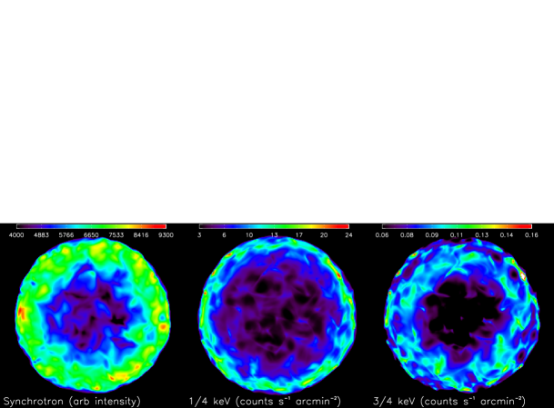
Figure 3: Three dimensional projection of emission onto the XY plane for (a) ROSAT $\text@frac{1}{4}$ keV band, (b) ROSAT $\text@frac{3}{4}$ keV band, and (c) synchrotron emission ($pB^{1.5}$). Note that the ROSAT $\text@frac{1}{4}$ keV emission is more confined to a thin shell, while the ROSAT $\text@frac{3}{4}$ keV emission and synchrotron emission is more uniformly distributed. There is some correlation between the synchrotron and X-ray emission. However, there does not appear to be very strong point-to-point correlation in any of the emission knots.

We have also calculated the X-ray and estimated synchrotron emissivities of the final time step for a three dimensional projection onto each of the three principal planes of the turbulent simulation. The X-ray emission is calculated assuming a plasma in ionization equilibrium with a thermal spectrum as calculated by Raymond & Smith (1977) folded through the ROSAT response function for the $\text@frac{1}{4}$ keV and $\text@frac{3}{4}$ keV emission bands. It is assumed that all three bands are optically thin so that the total emission may be obtained by summing the emissivities along each axis, without any optical depth effects. The results for the emission in the XY plane are shown in Figure 3. We found that the fluctuations are equally strong along all three projections both for the thermal and non-thermal emission maps. As a result, the presence of the additional uniform magnetic field leaves no imprint on the synchrotron emissivity. The $\text@frac{1}{4}$ keV emission has a fluctuating but fairly thin shell of emission, while the $\text@frac{3}{4}$ keV emission, while fainter, is much more distributed in projected radius. At this final timestep, the postshock temperature is sufficiently low that the X-ray emission comes primarily from a region somewhat back from the shock where the temperature is higher. This is truer yet for the 3/4 keV band. Inclusion of thermal conduction may fill the center further as in the study of W44 by Shelton et al (1999).

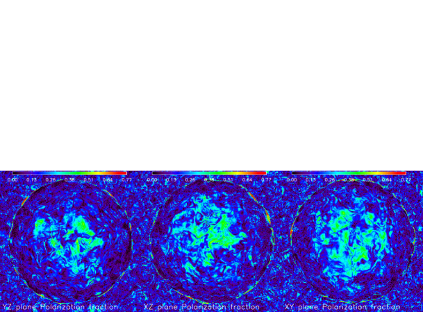
Figure 4: Synthetic synchrotron polarization maps showing the projections along the three principal axes at the same time step as Figure 3. The maximum polarization of the synchrotron emission is 0.77, corresponding to a electron energy power-law index of $p=2.5$. These images include the effects of Faraday rotation in the remnant and external medium for an observed frequency of 1 GHz. The turbulence considered here is sufficiently strong that a signature of the initially uniform field component does not show up in the polarization map at late times.

We have also calculated the polarization of the synchrotron emission as viewed along the three principal axes. We have assumed an electron energy spectrum with power-law index $p=2.5$, which implies a maximum linear polarization of 72% (Longair 1994). Figure 4 shows the result along all three axes for a frequency of $\nu=1$ GHz and includes Faraday rotation arising in both the remnant and the surrounding medium. We experimented with different frequencies and different levels of Faraday rotation in the surrounding medium. In all cases, we found that the level of turbulence we considered was large enough the signature of the initially uniform field component does not reveal itself in the polarization map that was made at a late time in the simulation. Comparing Figures 3 and 4, it is very interesting to note that the brightest emission features are also the most strongly polarized.

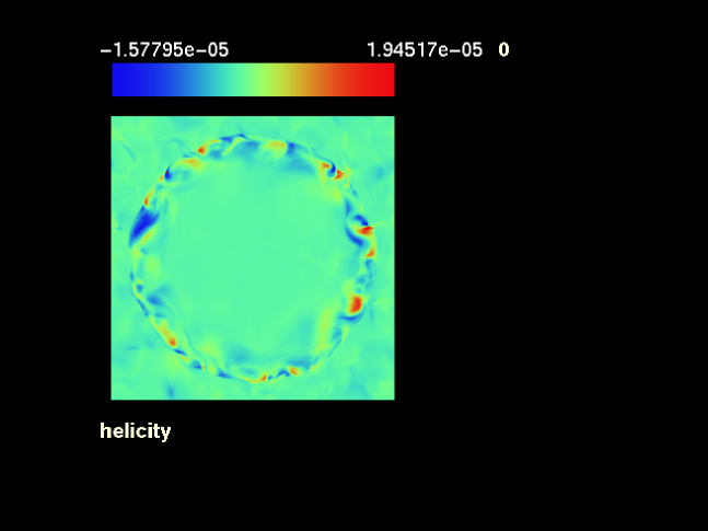
Figure 5: Color coded images for a two dimensional cut in the XZ plane showing the fluid’s helicity with both positive and negative values. The units are ${\rm cm/sec^{2}}$.

Several interesting points may be made about the interaction of turbulence with strong shocks. We focus here on one of the most interesting results, the generation of helicity at shocks. Figure 5 shows the fluid helicity in a cut in the XZ plane for the simulation where the SNR evolves in a turbulent medium. The lower right panel in Figure 1 shows the magnetic field strength in the same plane and at the same time. The propagation of the SNR shock through the interstellar turbulence has excited strong positive and negative helicity fluctuations in the post-shock region. An examination of the magnetic field strength shows that the field is strongest either in the regions with the highest helicity or in the regions where helicities of opposite signs closely abut one another. This positive correlation between helicity and magnetic field is consistent with the stretch, twist, fold scenario for magnetic field amplification that has been detailed in Childress & Gilbert (1995). Ferriere (1998) has presented a scenario in which supernovae interacting with galactic shear in a quiescent, stratified ISM could produce the helicity that is needed in dynamo theories. The present simulations suggest that interaction of strong supernova shocks with interstellar turbulence might be an additional and highly dynamic source of helicity generation and might, therefore, have relevance for fast dynamo theories.

4 Discussion

Supernova remnants serve as useful “test explosions” that can be used to probe the parameters characterizing the surrounding circumstellar and interstellar medium. These calculations inject an element of realism into the modelling of the pre-SNR environment that has heretofore been lacking, although much remains to be done. In a quiescent medium, we find that the remnant sweeps up the uniform field, and yields a bilateral morphology. The introduction of realistic, strongly turbulent fluctuations in the uniform medium, however, erases this asymmetry, and produces remnants that are (on average) spherical. The resulting projected X-ray and synchrotron maps show a range of fluctuation in the emission characteristics of the remnant.

We find that time variability and the angular variations in emission in the shell are associated with the nature of the magnetic fluctuations in the unshocked interstellar medium. We suggest, therefore, that it should be possible to use the variation in emission in the remnant as a probe of the turbulence in the pre-supernova environment. A grid of models like these will be needed to determine how the nature of the turbulence is related to the emission characteristics of the remnant.

Finally, we note that the interaction of SNR blastwave with a region of supersonic MHD turbulence gives an opportunity to investigate the degree to which magnetic fluctuations affect the effective equation of state of magnetized plasmas. The importance of understanding the nature of this behavior in interstellar conditions has been emphasized by McKee & Zweibel (1995). In future explorations, we will check to see how this effective equation of state varies over time with the parameters characterizing the MHD turbulence.

References

- Anderson (1996) Anderson, M.C. & Rudnick, L.,1996, ApJ, 456, 234
- Balsara (1998a) Balsara, D.S. 1998a, ApJS, 116, 119
- Balsara (1998b) Balsara, D.S. 1998b, ApJS, 116, 133
- Balsara (1998a) Balsara, D.S. 1999a, J. Quant. Spectros. Rad. Transf., 61, 617
- (5) Balsara, D.S. 1999b, J. Quant. Spectros. Rad. Transf., 61, 629
- (6) Balsara, D.S. 1999c, J. Quant. Spectros. Rad. Transf., 61, 637
- (7) Balsara, D.S. 1999d, J. Quant. Spectros. Rad. Transf., 62, 167
- (8) Balsara, D.S. 1999e, J. Quant. Spectros. Rad. Transf., 62, 225
- (9) Balsara, D.S. and Spicer, D.S. 1999a, J. Comput. Phys., 148, 133
- (10) Balsara, D.S. and Spicer, D.S. 1999b, J. Comput. Phys., 149, 270
- (11) Balsara, D.S. and Pouquet, A. 1999, Phys. Plas., 6, 89
- (12) Balsara, D.S. and Shu, C.-W. 2000, J. Comput. Phys., 160, 405
- (13) Balsara, D.S. 2000, in “Astrophysical Plasmas: Codes, Models, and Observations”, eds. S. J. Arthur, N. Brickhouse, and J. Franco, RevMexAA(SC), 9, 92.
- (14) Balsara, D.S., Crutcher, R.M. and Pouquet, A. 2001, ApJ, in press
- (15) Balsara, D.S. Ward-Thompson, D. and Crutcher, R.M. 2001, MNRAS, in press
- (16) Balsara, D.S. 2001a, ApJS, 132, 1
- (17) Balsara, D.S. 2001b, J. Quant. Spectros. Rad. Transf., 69(6), 671
- (18) Balsara, D.S. 2001c, J. Comput. Phys.,”Divergence-Free Adaptive Mesh Refinement for Magnetohydrodynamics”, submitted
- (19) Balsara, D.S. and Norton, C. 2001, Parallel Comput., 27, 37
- (20) Beck, R., 1991 in “ASP Conference Series Vol 18”, eds. N.Duric and P.C.Crane.
- (21) Beck, R.,Brandenburg,A., Moss,D.,Shukurov,A and Sokoloff,D.D., 1996, ARAA, 34, 155
- (22) Bisnovati-Kogan,G.S. and Silich,S.A., 1995, Rev. Modern Phys., 67, 661
- (23) Childress, S. and Gilbert, A.D. ,1995, ”Stretch Twist Fold : The Fast Dynamo”, Springer Lecture Notes in Physics
- (24) Cox, D. P., Shelton, R. L., Maciejewski, W., Smith, R. K., Plewa, T., Pawl, A., & Rozyczka, M., 1999, ApJ, 524, 179
- (25) Dickel, J.R., van Bruegel, W.R.J. & Strom, R.G., 1991, AJ, 101, 2151
- (26) Dohm-Palmer, R.C. and Jones, T.W., 1996, ApJ, 471, 279
- (27) Ferriere, K. , 1998, ApJ, 335, 488
- (28) Gaensler, B.M., 1998, ApJ, 493, 781
- (29) Jun, B.I. & Jones, T.W., 1999, ApJ, 511, 774
- (30) Kesteven, M.J. and Caswell, J.L., 1987, A&A, 183, 118
- (31) Lee, L.C. and Jokipii, J.R., 1976, ApJ, 206, 735
- (32) Longair, M.S. 1994, High Energy Astrophysics: Volume 2, (Cambridge: Cambridge University Press), 255
- (33) McKee, C.F. & Zweibel, E.G. 1995, ApJ, 40, 686
- (34) Reed, J.E., Hester, J., Fabian,A.C. and Winkler, P.F.,1995, ApJ, 440, 706
- (35) Reynolds, S.P. & Gilmore, D.M.,1993, AJ, 106,
- (36) Roe,P.L. and Balsara, D.S. 1996, SIAM J. Appl. Math., 56, 57
- (37) Shelton, R.L., 1999, ApJ, 521, 217
- (38) Shelton, R.L. et al. 1999, ApJ, 524, 179
- (39) Raymond, J.C. & Smith, B. 1977, ApJS, 35, 419