Applications of scalar attractor solutions to Cosmology

Abstract

We develop a framework to study the phase space of a system consisting of a scalar field rolling down an arbitrary potential with varying slope and a background fluid, in a cosmological setting. We give analytical approximate solutions of the field evolution and discuss applications of its features to the issues of quintessence, moduli stabilisation and quintessential inflation.

]

I Introduction

Scalar fields play a central role both in particle physics and cosmology. For example, in the Standard Model of particle physics, the Higgs boson generates particle masses through a mechanism of symmetry breaking. Supersymmetric models, believed to solve the hierarchy problem and to suggest a grand unification scale, add a whole new set of scalar (and fermionic) partners to the particles of the Standard Model. In string theories, the only physical constant is the string tension being all the other constants generated dynamically through scalar fields, the moduli.

In cosmology, a scalar field, the inflaton, has been suggested to be responsible for an early inflationary period in the history of the universe. This scenario can account for the extreme flatness and homogeneity of our Universe [4]. More recently, measurements of the apparent magnitude–redshift relation of type Ia supernovae (SnIa) support indications given by the combination of cosmic microwave background radiation (CMB), galaxy clusters and light elements abundances measurements, that the Universe is presently undergoing a period of accelerated expansion [5]. Once again, the existence of a scalar field rolling down a potential has been suggested as an explanation for this late inflationary period. The scalar field is usually called “quintessence” [6]. However, whether the inflaton and quintessence could be the same field, remains an interesting open question.

Considering these and other examples of applications of dynamical scalar fields in physics, it seems important to take a closer look to the features of their potentials.

For instance, in the issue of quintessence, if the potentials have attractor solutions (i.e. the late time dynamics is independent of the initial conditions) then there is a chance to weaken the fine tuning problem associated with a cosmological constant term in Einstein’s equations [7]. In the same way, when allowing for dynamical evolution of the moduli fields, the existence of attractor solutions opens up a larger region of initial conditions for which the fields can have successful stabilisation at their vacuum expectation value [8, 9].

The aim of this work is to extend the results of [10, 11, 12, 13] to more generic type of potentials, motivated by the issues of quintessence, moduli stabilisation and quintessential inflation and to give analytical support to some of the conclusions in [14].

II Setup

We consider a spatially–flat Friedmann–Robertson–Walker Universe containing a scalar field $\phi$ with potential $V(\phi)$, and a barotropic fluid with equation of state $p_{B}=(\gamma-1)\rho_{B}$, where $\gamma$ is a constant (e.g. $\gamma=4/3$ for radiation and $\gamma=1$ for matter). The governing equations of motion are,

$$\dot{H} = -\frac{\kappa^{2}}{2}\left(\gamma\rho_{B}+\dot{\phi}^{2}\right)\,,$$ (1)

$$\dot{\rho}_{B} = -3\gamma H\rho_{B}\,,$$ (2)

$$\ddot{\phi} = -3H\dot{\phi}-\frac{dV}{d\phi}\,,$$ (3)

subject to the Friedmann constraint

$$H^{2}=\frac{\kappa^{2}}{3}\left(\rho_{B}+\frac{1}{2}\dot{\phi}^{2}+V\right)\,,$$ (4)

where $\kappa^{2}=8\pi G$ and dots denote derivatives with respect to time. The energy density and pressure of a homogeneous scalar field are given by $\rho_{\phi}=\dot{\phi}^{2}/2+V$ and $p_{\phi}=\dot{\phi}^{2}/2-V$, respectively.

Following [12], we define the variables,

$$x\equiv\frac{\kappa\phi^{\prime}}{\sqrt{6}},\hskip 28.45274pty^{2}\equiv\frac{\kappa^{2}V}{3H^{2}},$$ (5)

where a prime denotes a derivative with respect to the logarithm of the scale factor $a$, $N\equiv\ln a$.

The effective equation of state for the scalar field at any point yields,

$$\gamma_{\phi}\equiv\frac{\rho_{\phi}+p_{\phi}}{\rho_{\phi}}=\frac{\dot{\phi}^{2}}{\dot{\phi}^{2}/2+V}=\frac{2x^{2}}{x^{2}+y^{2}},$$ (6)

constrained between $0\leq\gamma_{\phi}\leq 2$. In terms of these new variables the equations of motion read:

$$x^{\prime} = -3x+\lambda\sqrt{\frac{3}{2}}y^{2}+\frac{3}{2}x~{}[2x^{2}+\gamma(1-x^{2}-y^{2})]\,,$$ (7)

$$y^{\prime} = -\lambda\sqrt{\frac{3}{2}}xy+\frac{3}{2}y~{}[2x^{2}+\gamma(1-x^{2}-y^{2})]\,,$$ (8)

$$\lambda^{\prime} = -\sqrt{6}\lambda^{2}(\Gamma-1)x\,,$$ (9)

where we have defined

$$\lambda\equiv-\frac{1}{\kappa V}\frac{dV}{d\phi}\,,\hskip 28.45274pt\Gamma\equiv V\frac{d^{2}V}{d\phi^{2}}/\left(\frac{dV}{d\phi}\right)^{2}.$$ (10)

See [14] and [7] respectively, where these definitions were first introduced. Note that both $\lambda$ and $\Gamma$ are, in general, $\phi$ (and thus, time) dependent.

The contribution of the scalar field to the total energy density, $\Omega_{\phi}\equiv\kappa^{2}\rho_{\phi}/3H^{2}=x^{2}+y^{2}$ is bounded, $0\leq\Omega_{\phi}\leq 1$, if $\rho\geq 0$. Hence, the evolution of the system is completely described by trajectories within the unit circle. Moreover, since the system is symmetric under the reflection $(x,y)\rightarrow(x,-y)$ and time reversal $t\rightarrow-t$, we only consider the upper half disc, $y\geq 0$ in what follows.

For a generic scalar potential, one can identify up to five regions in the phase space diagram $(x,y)$. As an example, in Fig. 1 and Fig. 2 we show an exact numerical solution of the evolution of the system for a double exponential potential. In these figures, region 1 represents a regime in which the potential energy rapidly converts into kinetic energy; in region 2, the kinetic energy is the dominant contribution to the total energy density of the scalar field (“kination”); in region 3, the field remains nearly constant until the attractor solution is reached (“frozen field”); in region 4 the field evolves into the attractor solution, where the ratio of the kinetic to potential energy is a constant or slowly varying; and in region 5 the potential energy becomes important, the scalar field dominates and drives the dynamics of the Universe.

In section III we will briefly discuss regions 1, 2, and 3. However, in this paper we will be mostly concerned with regions 4 and 5 of the evolution since (as it will be shown) they correspond to stable solutions yet not having true critical points associated with them. As we will see, this feature plays an important role in many cosmological phenomena.

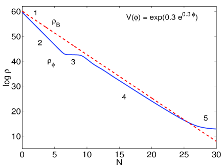
FIG. 1.: Evolution of the scalar field energy density $\rho_{\phi}$ in a radiation background fluid $\rho_{B}$ for a double exponential potential. Regions 2 to 5 represent respectively, kination, frozen field, evolution in the attractor and scalar field domination.

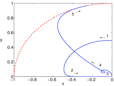
FIG. 2.: The scalar field dynamics in the phase space diagram for a double exponential potential. Regions 1 to 5 are the same as in Fig. 1. The dashed line represents the unit circle $x^{2}+y^{2}=1$.

III Early Evolution

For a wide range of potentials (including the potential in Figs. 1 and 2), when $\phi$ is high up the potential slope at the beginning of the cosmological evolution, then $\lambda$ is large initially. The behaviour of the trajectory close to the $\lambda=\infty$ surface can be deduced by continuity from the $\lambda=\infty$ solution, even though the latter is not physical.

We bring the plane $\lambda=\infty$ to a finite distance from the $\lambda=0$ plane by the transformation

$$\lambda={\delta\over 1-\delta}\ ,\hskip 28.45274pt0\leq\delta\leq 1\ ,$$ (11)

so that the $\delta=0$ surface corresponds to the $\lambda=0$ surface and the $\delta=1$ surface corresponds to $\lambda=\infty$. On the plane $\delta=1$, we find

$$\frac{dx}{d\tau}=\sqrt{3\over 2}y^{2}\,,\hskip 28.45274pt\frac{dy}{d\tau}=-\sqrt{3\over 2}xy\,$$ (12)

where $\tau$ is a new time coordinate defined by $d\tau=\lambda dN$ [15].

Solving Eqs. (12), we obtain,

$$x = A\tanh\left[\sqrt{3\over 2}(\tau-\tau_{0})\right]\ ,$$ (13)

$$y = A\mbox{ sech}\left[\sqrt{3\over 2}(\tau-\tau_{0})\right]\ ,$$ (14)

where $A$ and $\tau_{0}$ are arbitrary constants.

As shown in Fig. 2, the trajectory for region 1 is nearly circular, well described by Eqs. (13) and (14). For $\lambda$ very large, the scalar field potential energy turns into kinetic energy very rapidly.

In region 2, the trajectory is very close to the $x$–axis where the scalar field energy density is kinetic energy dominated (hence $y\approx 0$), and its behaviour in the $x$ direction is described by

$$x^{\prime}=-{3\over 2}(2-\gamma)x(1-x^{2})\ .$$ (15)

For $x<0$, $x^{\prime}$ is always positive and $x$ increases; for $x>0$, $x^{\prime}$ is always negative and $x$ decreases bringing the trajectory towards the $\lambda$ – axis (in the $3$–dimensional phase space ($x,y,\lambda$)).

Close to the $\lambda$–axis, the system is described by

$$x^{\prime}=-{3\over 2}(2-\gamma)x\,,\hskip 28.45274pty^{\prime}=\frac{3}{2}\gamma y\,.$$ (16)

Therefore, the trajectory in region 3 evolves along the $x$ direction at a rate of $x\propto a^{-3(2-\gamma)/2}$. Since the background fluid is dominant at this stage, $H^{2}\propto a^{-3\gamma}$, we have the kinetic energy falling off rapidly as $\dot{\phi}^{2}\sim x^{2}H^{2}\propto a^{-6}$. The trajectory moves in the $y$ direction as $y\propto a^{3\gamma/2}$, that is $V\sim y^{2}H^{2}\approx\mbox{constant}$ and the scalar field is essentially “frozen”.

IV The tracker solution

In this section we study the case in which the scalar field evolution is well approximated by a linear relation between $x$ and $y$, as it happens along region 4 of the example illustrated in Fig. 2. In order to study the evolution of the scalar field when the slope of the potential is varying, i.e. $\lambda$ is changing with time, we rewrite Eqs. (7) by defining $\epsilon=1/\lambda$, $x=\epsilon X$, and $y=\epsilon Y$.

We then have,

$$X^{\prime} = \sqrt{6}(\Gamma-1)X^{2}-3X+\sqrt{\frac{3}{2}}Y^{2}+\,$$ (17)

$$\frac{3}{2}X[2\epsilon^{2}X^{2}+\gamma(1-\epsilon^{2}X^{2}-\epsilon^{2}Y^{2})]\,,$$ (18)

$$Y^{\prime} = \sqrt{6}(\Gamma-1)XY-\sqrt{\frac{3}{2}}XY+\,$$ (19)

$$\frac{3}{2}Y[2\epsilon^{2}X^{2}+\gamma(1-\epsilon^{2}X^{2}-\epsilon^{2}Y^{2})]\,,$$ (20)

$$\epsilon^{\prime} = \sqrt{6}\epsilon(\Gamma-1)X\,.$$ (21)

For $\epsilon$ small ($\lambda$ large) or $\Gamma\approx 1$, $\epsilon$ becomes nearly constant. Moreover, if $\Gamma$ is also nearly constant we can solve $X^{\prime}=Y^{\prime}=0$ and find the “instantaneous critical points”,

$$x_{c}(\lambda)=\sqrt{\frac{3}{2}}\frac{\gamma_{\phi}}{\lambda}\,,\hskip 28.45274pty_{c}^{2}(\lambda)=\frac{3}{2}\frac{\gamma_{\phi}}{\lambda^{2}}(2-\gamma_{\phi})\,,$$ (22)

where the equation of state of the scalar field is

$$\gamma_{\phi} = \frac{1}{2}[\gamma+(2\Gamma-1)\lambda^{2}/3]\pm\,$$ (23)

$$\frac{1}{2}\sqrt{\left[-\gamma+(2\Gamma-1)\lambda^{2}/3\right]^{2}+8\gamma(\Gamma-1)\lambda^{2}/3}\,.$$ (24)

The plus root leads to unphysical results, so only the negative one will be used in what follows. The contribution of the field to the total energy density is $\Omega_{\phi}=3\gamma_{\phi}/\lambda^{2}$.

Note that in the limit when $\Gamma-1\approx 0$ one has

$$\gamma_{\phi}=\gamma\left[1-\frac{2(\Gamma-1)}{1-3\gamma/\lambda^{2}}\right]\,.$$ (25)

In other words, for potentials with small curvature, the equation of state of the scalar field is very close to the equation of state of the background fluid, and it is said that the field “tracks” the background fluid. This expression can account for values of $\Omega_{\phi}>1/2$.

From Eq. (23), it can also be shown that in the limit of large $\lambda$, when the background fluid is completely dominating, we recover the expression in [7],

$$\gamma_{\phi}=\frac{\gamma}{2\Gamma-1}.$$ (26)

In the limit when $\Gamma-1\approx 0$, the above expression is equivalent to Eq. (25) in the limit of large $\lambda$.

One can now study the stability of the “instantaneous critical points” linearising Eqs. (17) in $u$ and $v$ with $X=X_{c}+u$ and $Y=Y_{c}+v$ resulting in the first-order equations of motion,

$$\left(\begin{array}[]{c}u^{\prime}\\ v^{\prime}\end{array}\right)=\mathcal{M}\left(\begin{array}[]{c}u\\ v\end{array}\right).$$ (31)

Using Eq. (23) to write $\Gamma-1$ in terms of $\gamma_{\phi}$, we find the eigenvalues,

$$m_{\pm}=-\frac{3}{4\lambda^{2}}\left[(\gamma-\gamma_{\phi})(3\gamma_{\phi}+\lambda^{2})+(2-\gamma_{\phi})\lambda^{2}\right]\times\,$$ (32)

$$\left[1\pm\sqrt{1-\frac{8~{}\lambda^{2}(2-\gamma_{\phi})(\gamma\lambda^{2}-3\gamma_{\phi}^{2})}{[(\gamma-\gamma_{\phi})(3\gamma_{\phi}+\lambda^{2})+(2-\gamma_{\phi})\lambda^{2}]^{2}}}~{}\right]\,.$$ (33)

It is straightforward to check that Eq. (32) reduces to Eq. (A8) of [12] when $\gamma=\gamma_{\phi}$ (i.e. the pure exponential case) and to Eq. (15) of [7] in the limit of large $\lambda$.

The system is stable if the real part of both eigenvalues is negative. From Eq. (32), this is completely assured if,

$$\gamma_{\phi} < \sqrt{\frac{\gamma\lambda^{2}}{3}}\,,{~{}~{}~{}\rm and}$$ (34)

$$\gamma_{\phi} < \frac{3\gamma-2\lambda^{2}}{6}\left(1-\sqrt{1+\frac{12\lambda^{2}(2+\gamma)}{(3\gamma-2\lambda^{2})^{2}}}~{}\right)\,.$$ (35)

Moreover, if the quantity under the square root of Eq. (32) is negative, the critical points are a stable spiral; and a stable node, otherwise. In Fig. 3 and Fig. 4 one can see the dependence of the eigenvalues on $\gamma_{\phi}$ and $\lambda$ for a background fluid of matter ($\gamma=1$) and radiation ($\gamma=4/3$), respectively. The lines split when the quantity under the square root of Eq. (32) becomes positive. The first of the conditions in Eqs. (34) marks the point for which only one of the real parts of the eigenvalues becomes positive, and the second condition the point where both real parts of the eigenvalues become positive. In the limit of large $\lambda$ the latter is $\gamma_{\phi}=1+\gamma/2$.

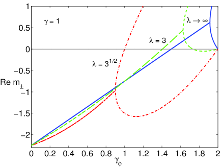
FIG. 3.: Dependence of the real part of the eigenvalues on $\gamma_{\phi}$ and $\lambda$ for a background fluid of matter. Upper and lower lines represent respectively solutions $-$ and $+$ in Eq. (32).

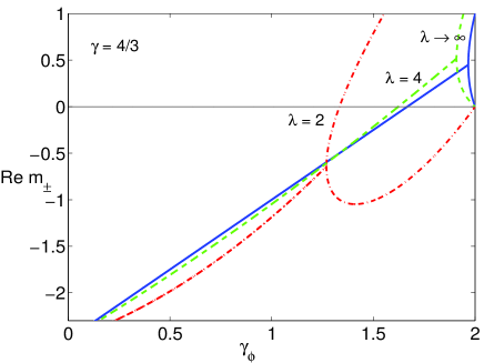
FIG. 4.: Dependence of the real part of the eigenvalues on $\gamma_{\phi}$ and $\lambda$ for a background fluid of radiation. Upper and lower lines represent respectively solutions $-$ and $+$ in Eq. (32).

For a large class of scalar potentials $V(\phi)$, stability is possible for a large number of $e$-folds allowing a scalar field sub-dominance during a long period of time as we will see in the applications below. We should point out that so far these results are general since we have not assumed, yet, any type of potential $V(\phi)$.

V The scalar field dominated solution

We now consider the case in which the evolution of the scalar field approaches the unit circle $x^{2}+y^{2}=1$, as it is the case along region 5 of Fig. 2. Introducing the new variables $x=\lambda X$ and $y^{2}=1-\lambda^{2}Y^{2}$, Eqs. (7) give,

$$X^{\prime} = \sqrt{6}\lambda^{2}(\Gamma-1)X^{2}-3X+\sqrt{\frac{3}{2}}(1-\lambda^{2}Y^{2})^{2}+\,$$ (36)

$$\frac{3}{2}\lambda^{2}X[2X^{2}+\gamma(-X^{2}+Y^{2})]\,,$$ (37)

$$YY^{\prime} = \sqrt{6}\lambda^{2}(\Gamma-1)XY^{2}+\sqrt{\frac{3}{2}}X(1-\lambda^{2}Y^{2})-\,$$ (38)

$$\frac{3}{2}(1-\lambda^{2}Y^{2})[2X^{2}+\gamma(-X^{2}+Y^{2})]\,.$$ (39)

However, the same kind of analysis as for the tracker solution becomes here extremely complicated. We take then a set of simple reasonable assumptions in order to obtain simple and useful results.

One can see from Fig. 2 that at late times, when the scalar field is dominant, $y$ is approximately $1$ and $x$ approaches zero. This means the scalar potential is overtaking the energy density and the potential is very flat. In other words, $\lambda$ is getting closer to zero. Let us take then $\lambda\approx 0$ and $\lambda^{2}(\Gamma-1)$ nearly constant. Eq. (36) then reads,

$$X^{\prime} = \sqrt{6}\lambda^{2}(\Gamma-1)X^{2}-3X+\sqrt{\frac{3}{2}}\,,$$ (40)

$$YY^{\prime} = \sqrt{6}\lambda^{2}(\Gamma-1)XY^{2}+\sqrt{\frac{3}{2}}X-\,$$ (41)

$$\frac{3}{2}[2X^{2}+\gamma(-X^{2}-Y^{2})]\,.$$ (42)

The system has critical points in,

$$x_{c}(\lambda)=\frac{\lambda_{\phi}}{\sqrt{6}}\,,\hskip 28.45274pty_{c}^{2}(\lambda)=1-\frac{\lambda_{\phi}^{2}}{6}\,.$$ (43)

Hence, the scalar field is dominant, $\Omega_{\phi}=1$ and $\gamma_{\phi}=\lambda_{\phi}^{2}/3$, where we have defined

$$\lambda_{\phi}=\frac{3}{2}\left[\frac{1\pm\sqrt{1-4(\Gamma-1)\lambda^{2}/3}}{(\Gamma-1)\lambda}\right],$$ (44)

for $\Gamma\neq 1$, and $\lambda_{\phi}=\lambda$ otherwise. As before, only the minus solution has physical meaning. Expanding $\lambda_{\phi}$ we can approximate the solution by

$$\lambda_{\phi}=\lambda\left[1+\frac{1}{3}(\Gamma-1)\lambda^{2}\right]\,.$$ (45)

As we did for the tracker solution, we perturb the solutions around the critical points to study their stability. Expanding Eq. (36) and using Eq. (44) to write $\Gamma-1$ in terms of $\lambda$ and $\lambda_{\phi}$, we find the following eigenvalues:

$$m_{+} = 6~{}(\lambda_{\phi}-\lambda)\frac{1}{\lambda_{\phi}}+\frac{1}{2}(\lambda_{\phi}^{2}+\lambda\lambda_{\phi}-6\gamma)\,,$$ (46)

$$m_{-} = 3-6~{}\frac{\lambda}{\lambda_{\phi}}+\frac{1}{2}\lambda_{\phi}(3\lambda_{\phi}-2\lambda)\,.$$ (47)

For $\Gamma=1$ this expression reduces to the eigenvalues found in [12], as we would expect. In Fig. 5 and Fig. 6 we show the dependence of the eigenvalues on $\gamma_{\phi}$ and $\lambda$ for a background fluid of matter and radiation, respectively.

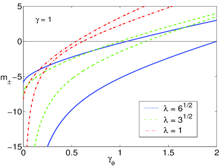
FIG. 5.: Dependence of the eigenvalues on $\gamma_{\phi}$ and $\lambda$ for a background fluid of matter. Upper and lower lines represent respectively solutions $m_{+}$ and $m_{-}$ in Eq. (46).

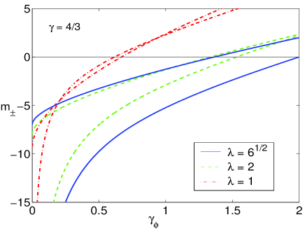
FIG. 6.: Dependence of the eigenvalues on $\gamma_{\phi}$ and $\lambda$ for a background fluid of radiation. Upper and lower lines represent respectively solutions $m_{+}$ and $m_{-}$ in Eq. (46).

For completeness, we indicate that the background fluid dominated solution with $(x,y,\lambda)=(0,0,\lambda)$ has eigenvalues,

$$m_{+}=\frac{3\gamma}{2}\,,\hskip 28.45274ptm_{-}=-\frac{3(2-\gamma)}{2}\,,$$ (48)

and when $\Gamma=1$, there exist the kinetic dominated solutions $(x,y,\lambda)=(\pm 1,0,\lambda)$ with eigenvalues,

$$m_{+}=3~{}(2-\gamma)\,,\hskip 14.22636ptm_{-}=\sqrt{\frac{3}{2}}~{}(\sqrt{6}\mp\lambda)\,.$$ (49)

In Table I we give a summary of the properties of these critical points.

$x_{c}$	$y_{c}^{2}$	Existence	Stability	$\Omega_{\phi}$	$\gamma_{\phi}$
$0$	$0$	all $\gamma$ and $\lambda$	saddle point for $0<\gamma<2$	$0$	undefined
$1$	$0$	all $\gamma$ and $\lambda$	unstable node for $\lambda<\sqrt{6}$,  saddle point for $\lambda>\sqrt{6}$	$1$	$2$
$-1$	$0$	all $\gamma$ and $\lambda$	unstable node for $\lambda>-\sqrt{6}$,  saddle point for $\lambda<-\sqrt{6}$	$1$	$2$
$\sqrt{\frac{3}{2}}\frac{\gamma_{\phi}}{\lambda}$	$\frac{3}{2}\frac{\gamma_{\phi}}{\lambda^{2}}(2-\gamma_{\phi})$	$\lambda^{2}>3\gamma_{\phi}$	stable for $Re(m_{\pm})<0$ (see Eq. (32))	$\frac{3\gamma_{\phi}}{\lambda^{2}}$	Eq. (23)
$\frac{\lambda_{\phi}}{\sqrt{6}}$	$1-\frac{\lambda_{\phi}^{2}}{6}$	$\lambda_{\phi}^{2}<6$	stable for $m_{\pm}<0$ (see Eq. (46))	$1$	$\frac{\lambda_{\phi}^{2}}{3}$

TABLE I.: The properties of the critical points. $\lambda_{\phi}$ is defined in Eq. (44).

VI Applications

A Quintessence

The first estimate for the value of the cosmological constant from current particle physics is the Planck scale, while the lowest is set by the electroweak scale, namely, of order $10^{8}~{}{\rm GeV}^{4}$. These are tremendously high values on cosmological energy scales. So, the simplest solution so far has been to assume that by some mechanism, the cosmological constant would vanish altogether.

In the last decade, measurements of the apparent magnitude–redshift relation using SnIa combined with CMB and galaxy clusters and light elements abundances measurements, give indications that we are living in an accelerating Universe with $\Omega_{\rm matter}\sim 0.3$ and $\Omega_{\Lambda}\sim 2/3$ [5]. Then, the discovery that the cosmological constant like term is small but non zero, is disturbing. Having today a cosmological constant energy density contribution, $\rho_{\Lambda}=\Lambda/8\pi G$, of the same order of magnitude as the critical energy density $\rho_{c}\sim 10^{-47}{\rm GeV}^{4}$, requires to fine tune its initial value to 120 orders of magnitude below the Planck scale. In order to alleviate this puzzle, the idea of “quintessence” was introduced [6]. One of its versions consistes of an inhomogeneous scalar field $Q$ rolling down a potential with attractor solutions. The argument is that if the scalar field joins the attractor solution before the present epoch, information about the initial conditions will get lost, which allows a freedom in choosing those conditions within 100 orders of magnitude, thus relieving the fine tuning issue. The initial suggestion for such potentials was to use an inverse power law form $V(Q)\propto Q^{-\alpha}$ which can be found in models of supersymmetric QCD [16]. Pure exponential potentials $V\propto\exp(\lambda Q)$ also have attractor solutions; however, they cannot be used on their own to model quintessence [17] but interesting modifications have been proposed such as $V\propto\exp(-\lambda Q)Q^{-\alpha}$ [18], sum of pure exponentials $V\propto\exp(\alpha Q)+\exp(\beta Q)$ [19], Supergravity inspired models with $V\propto\exp(Q^{2})Q^{-\alpha}$ [20] or $V\propto\exp(Q^{4/3})Q^{2/3}$ [21].

In this section we will give the scalar field and its equation of state evolution in a background fluid dominated setting, for the inverse power law potential. We will then turn to the general potential $V\propto\exp(\alpha Q^{\beta})Q^{\mu}$.

Consider the inverse power law potential,

$$V(Q)=\frac{M^{4+\alpha}}{Q^{\alpha}}\,.$$ (50)

for which the relevant quantities are

$$\lambda=-\frac{\alpha}{\kappa Q},~{}~{}~{}~{}~{}\Gamma-1=\frac{1}{\alpha}\,.$$ (51)

We have seen in section IV that when the background fluid is dominant the equation of state of the scalar field can be well approximated by Eq. (26). Therefore, in this case the equation of state is a constant and is given by

$$\gamma_{Q}=\frac{\gamma\alpha}{2+\alpha}.$$ (52)

Integrating the $x$ equation in Eq. (22) the solution for the scalar field reads,

$$Q=Q_{i}\left(\frac{a}{a_{i}}\right)^{3\gamma/(2+\alpha)},$$ (53)

where $Q_{i}$ can be derived from the $y$ equation assuming $H^{2}\approx\kappa^{2}/3~{}\rho_{B}^{i}\exp(-3\gamma N)$, with $N=\ln(a/a_{i})$, to give

$$Q_{i}=\left[\frac{3}{2}\frac{\kappa^{2}\rho_{B}^{i}}{M^{4+\alpha}}\frac{\gamma_{Q}(2-\gamma_{Q})}{\alpha^{2}}\right]^{-1/(2+\alpha)}.$$ (54)

We review here some of the properties of power law type of potentials [11]. For example, Eq.(52) still holds for negative $\alpha$ provided $\alpha<-2$. Moreover, we have seen that for large $\lambda$, the solutions are stable provided $\gamma_{Q}<1+\gamma/2$, which yields,

$$\alpha > 2\frac{\gamma+2}{\gamma-2},\hskip 28.45274pt\alpha>0\,,$$ (55)

$$\alpha < 2\frac{\gamma+2}{\gamma-2},\hskip 28.45274pt\alpha<0\,.$$ (56)

For $\alpha>0$ the condition is always true, however, for $\alpha<0$ it imposes the bounds $\alpha<-6$ and $\alpha<-10$ for matter and radiation dominated fluids, respectively. For even, negative $\alpha$ the field can have early oscillatory behaviour with average equation of state given by the virial theorem

$$<\gamma_{Q}>=1+\frac{\alpha+2}{\alpha-2},$$ (57)

while energy is continually being converted between kinetic and potential.

Consider now the more general potential,

$$V(Q)=M^{4}e^{\alpha(\kappa Q)^{\beta}}(\kappa Q)^{\mu}\,;$$ (58)

we have

$$\lambda = -(\alpha\beta(\kappa Q)^{\beta}+\mu)(\kappa Q)^{-1}\,,$$ (59)

$$\Gamma-1 = \frac{\alpha\beta(\beta-1)(\kappa Q)^{\beta}-\mu}{(\alpha\beta(\kappa Q)^{\beta}+\mu)^{2}}$$ (60)

and integrating $x$ in Eq. (22) with $\gamma_{\phi}$ given by Eq. (26), we find the solution

$$\alpha(\kappa Q)^{\beta} = \Phi_{i}+\frac{2-\mu}{\beta}\ln(\kappa Q)^{\beta}\,$$ (61)

$$- 2\ln[\alpha\beta(\kappa Q)^{\beta}+\mu]-3\gamma N\,,$$ (62)

where the last logarithm term only exists if $\alpha\neq 0$. $\Phi_{i}$ is an integration constant and can be derived from the $y$ equation. If we assume $\kappa Q\gg\mu/\alpha\beta$ then we have a nearly constant $\Gamma-1\approx 0$, and we can neglect this contribution from the equation of state, to yield the simple result,

$$\Phi_{i}=\ln\left[\frac{3}{2}\frac{\rho_{B}^{i}}{M^{4}}\gamma(2-\gamma)\right].$$ (63)

Since we do not have an explicit expression for $(\kappa Q)^{\beta}$ we take the ansatz used in [8], which is a perturbative solution,

$$\alpha(\kappa Q)^{\beta}_{1} = \Phi_{i}-3\gamma N\,,$$ (64)

$$\alpha(\kappa Q)^{\beta}_{n} = \Phi_{i}+\frac{2-\mu}{\beta}\ln(\kappa Q)^{\beta}_{n-1}\,$$ (65)

$$- 2\ln[\alpha\beta(\kappa Q)^{\beta}_{n-1}+\mu]-3\gamma N,$$ (66)

Substituting this solution back in Eqs. (59) and (26) we have now the complete evolution of the scalar field equation of state in terms of the background fluid energy density and model parameters, only. We can see from Fig. 7 that the second order solution is, in general, already a good approximation.

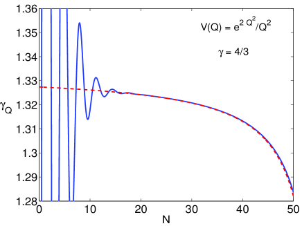
FIG. 7.: Evolution of the equation of state of the scalar field in a radiation background. The solid line is the numerical evolution and the dashed line our approximate analytical solution using Eqs. (64), (59) and (26).

Note that for a pure exponential ($\beta=1$, $\mu=0$), we recover the exact solution

$$Q=Q_{i}-\frac{3\gamma}{\kappa\alpha}N,$$ (67)

where $Q_{i}=\Phi_{i}/\kappa\alpha$.

When $\kappa Q\ll\mu/\alpha\beta$, a positive definite potential, Eq. (58) becomes well approximated by a pure power law potential, i.e. $\Gamma-1\approx-1/\mu$, $\alpha\approx 0$ and, neglecting the second logarithm contribution, we rewrite Eq. (61) as,

$$\kappa Q=\Psi_{i}~{}\left(\frac{a}{a_{i}}\right)^{3\gamma/(2-\mu)}\,,$$ (68)

where $\Psi_{i}=\exp(\Phi_{i}/(\mu-2))$, is estimated, as before, using the $y$ equation to yield,

$$\Psi_{i}=\left[\frac{3}{2}\frac{\rho_{B}^{i}}{M^{4}}\frac{1}{\mu^{2}}\frac{\gamma\mu}{\mu-2}\left(2-\frac{\gamma\mu}{\mu-2}\right)\right]^{-1/(2-\mu)}\,.$$ (69)

Despite the above solution being merely an approximation, substituting back in Eq. (59), the variation of the equation of state with time can be well accounted for.

B Moduli stabilisation

In string theory, the modulus and the dilaton (moduli) play an important role. They parametrise the structure of the compactified manifold and their vacuum expectation value (vev) determine the $d=4$ value of the gauge and gravitational couplings and fix the unification scale $M_{\rm GUT}$.

Stabilisation of the moduli fields in the $d=4$ effective theory, has been studied by including nonperturbative effects such as multiple gaugino condensates, which develop a minimum, and non-perturbative corrections to the Kähler potential [22]. Unfortunately, the scalar potentials in these theories are exponentially steep, therefore, it is expected that these fields roll past the minimum rather than acquiring a vev [23]. Hence, stabilisation of the moduli is one of the most serious questions in string theory. Solutions to this problem have been suggested in the literature. One possibility is that matter fields other than the moduli drive the evolution of the Universe [8, 9]. If this is the case, it has been shown that this setting opens up a wider region of the parameter space for which dynamical stabilisation of the moduli is successful. The reason behind this feature is, once again, the existence of attractor solutions that slow down the fields by the amount needed to trap them when they reach the minimum.

Away from the minimum, the evolution of the moduli can be written in terms of a canonically normalised field $\sigma$, in a double exponential potential.

We take the general potential

$$V(\sigma)=M^{4}\exp(\alpha e^{\beta\kappa\sigma}),$$ (70)

where $\alpha$ is an arbitrary real number. Following the same line of argument as before, we find the solution for $S\equiv\alpha\exp(\beta\kappa\sigma)$ to be (in accordance with [8]),

$$S_{1} = \Phi_{i}-3\gamma N\,,$$ (71)

$$S_{n} = \Phi_{i}-2\ln(S_{n-1}/\alpha)-3\gamma N,$$ (72)

and $\Phi_{i}$ is given by

$$\Phi_{i}=\ln\left[\frac{3}{2}\frac{\rho_{B}^{i}}{M^{4}}\frac{\gamma(2-\gamma)}{\alpha^{2}\beta^{2}}\right].$$ (73)

This attractor solution enables us to stabilise the dilaton at the minimum. One sees that the equation of state of the scalar field is the same as that of the background fluid, apart from a logarithmic deviation and an upper or lower shift given by $\Phi_{i}$. In other words, the ratio between kinetic and potential energy of the scalar field is roughly a constant and hence prevents the field from rolling past the minimum for certain values of the background fluid equation of state.

A last remark is that if $\alpha$ is positive, then $\lambda$ is decreasing and this becomes a realistic quintessence potential, as well.

C Quintessential inflation

We have seen in section V that for small enough values of $\lambda_{\phi}$ the scalar field drives the dynamics of the Universe. In this section we present scalar field dominated solutions for the same potentials used above. The particular case of $\lambda_{\phi}<2$ is of extreme importance, since it corresponds to an inflationary scenario ($\ddot{a}\propto-\rho_{\phi}-3p_{\phi}>0$). In what follows we consider a good approximation, taking $\lambda_{\phi}\approx\lambda$.

Considering the limit $(\kappa Q)^{\beta}\gg\mu/\alpha\beta$, we integrate $x$ in Eq.(43) to obtain for the potential $V(Q)=M^{4}\exp(\alpha(\kappa Q)^{\beta})(\kappa Q)^{\mu}$ the solution,

$$(\kappa Q)^{\beta}=\left[(\kappa Q_{i})^{2-\beta}+\alpha\beta(2-\beta)N\right]^{\beta/(2-\beta)}\,,$$ (74)

when $\beta\neq 2$, and

$$(\kappa Q)^{2}=-\frac{\mu}{\alpha\beta}+\left[(\kappa Q_{i})^{2}+\frac{\mu}{\alpha\beta}\right]\left(\frac{a}{a_{i}}\right)^{-2\alpha\beta}\,,$$ (75)

otherwise (see also [24]). The case $(\kappa Q)^{\beta}\ll\mu/\alpha\beta$ can be well approximated by the power law solution,

$$(\kappa Q)^{\beta}=\left[(\kappa Q_{i})^{2}-2\mu N\right]^{\beta/2}\,.$$ (76)

From Eq. (59), it should be clear that for $(\kappa Q)^{\beta}\gg\mu/\alpha\beta$, if $\beta<1$, $\lambda$ is increasing and we can imagine a scenario in which the Universe is first inflating and then, when $\lambda$ is such that $\lambda^{2}>2$ the universe starts to decelerate. Reheating can happen by gravitational particle production by which conventional particles are created quantum mechanically from the time varying gravitational field [25]. Moreover, if we choose negative $\mu$, the potential has a minimum with non vanishing vacuum energy. Assuming this minimum is the responsible for the currently accelerated expansion of the universe, we can envisage a scenario of “quintessential inflation” [26].

Taking the number of e-folds from the end of inflation to be $N=50$ and imposing the spectral index to be $n_{\rm S}>0.95$, a closer look at this potential reveals that

$$\beta<0.01,$$ (77)

and for the approximation $(\kappa Q)^{\beta}\gg-\mu/\alpha\beta$ to be valid,

$$-0.1\lesssim\mu<0.$$ (78)

The amplitude of density perturbations $A_{\rm S}=2\times 10^{-5}$ measured by COBE, then imposes

$$\alpha>293.8~{},\hskip 28.45274ptM<10^{-17}{\rm GeV}.$$ (79)

The ratio of tensorial to scalar perturbations is then, $A_{\rm T}^{2}/A_{\rm S}^{2}<0.17$, and the tensorial spectral index $n_{\rm T}>-0.028$.

An important condition in order not to spoil nucleosynthesis is that the value of the Hubble constant when inflation ends must be $H_{\rm end}>10^{8}{\rm GeV}$ which is amply satisfied in this model as $H_{\rm end}>10^{12}{\rm GeV}$.

For the double exponential potential, $V(\phi)=M^{4}\exp(\alpha e^{\beta\kappa\phi})$ the field rolls according to

$$\phi=-\frac{1}{\kappa\beta}\ln\left(e^{-\beta\kappa\phi_{i}}-\alpha\beta^{2}N\right)\,.$$ (80)

When $\alpha$ is negative the potential offers a plateau for $\beta\phi<0$, where inflation can happen. Assuming that particles are produced gravitationally as above, to satisfy the value of density perturbations we find, $M\approx 10^{15}{\rm GeV}$ and $n_{\rm S}\approx 0.96$. Furthermore, for $|\beta|>1$, these numbers are nearly independent of the precise values of $\alpha$ and $\beta$. We must also require, $\beta>0.1$ in order not to spoil nucleosynthesis predictions. As noted in [14], even if the field would reach the tracker solution before today, its contribution to the total energy density would be ever decreasing. So the scalar field can never explain, in this case, the present acceleration, unless some other contribution is added to the potential to make the scalar field become dominant today.

Although interesting, most of these models of quintessential inflation lead to a regime where the kinetic energy is the dominant contribution to the scalar field energy density until its value is of order the critical energy density today. Therefore, the contribution of the scalar field at the time of recombination is negligible and the value of the field equation of state today is very close to the one of the cosmological constant, $\gamma_{\Lambda}=0$. Hence, it is not expected that CMB and SnIa observations will be able to provide direct evidence for these scenarios. A second problem associated with these models is the overproduction of gravitinos, as the reheating temperature $T_{\rm RH}$ is often $T_{\rm RH}\sim H_{\rm end}\gtrsim 10^{9}~{}{\rm GeV}$, leading to dangerous cosmological consequences [27]. And of course, a solid theoretical motivation for the suggested phenomenological potentials is still to be found.

VII Summary

We have studied the dynamics of a scalar field in a flat FRW Universe with a barotropic fluid. We have considered the general case of field dependent slope $\lambda$ of the scalar potential and analysed the differences, especially in the stability conditions, with respect to the constant slope case. These results are summarised in table I. We exemplified the tracker and scalar field dominated solutions by giving explicit calculations of the field evolution for different potentials. We have discussed applications of these solutions to the issues of quintessence, moduli stabilisation and quintessential inflation. Finally, we would like to emphasise that we have demonstrated here the existence and stability of a number of scalar attractor solutions which have been previously only assumed in the literature.

- [1] E–mail: cng@physics.adelaide.edu.au
- [2] E–mail: kap13@pact.cpes.susx.ac.uk
- [3] E–mail: francesca.rosati@pd.infn.it
- [4] A. H. Guth, Phys. Rev. D23, 347 (1981).
- [5] A. G. Riess, et al., AJ 116, 1009 (1998); S. Perlmutter, et al., ApJ 517, 565 (1999); N. A. Bahcall, J. P. Ostriker, S. Perlmutter and P. J. Steinhardt, Science 284, 1481 (1999); P. de Bernardis et al., Nature 404, 955 (2000); A. Balbi, et al., ApJ 545, L1 (2000); C. B. Netterfield, astro-ph/0104460.
- [6] M. S. Turner and M. White, Phys. Rev. D56, 4439 (1997); J. A. Frieman and I. Waga, Phys. Rev. D57, 4642 (1998); R. R. Caldwell, R. Dave, and P. J. Steinhardt, Phys. Rev. Lett. 80, 1582 (1998); I. Zlatev, L. Wang, and P. J. Steinhardt, Phys. Rev. Lett. 82, 896 (1999).
- [7] P. J. Steinhardt, L. Wang, and I. Zlatev, Phys. Rev. D59, 123504 (1999).
- [8] T. Barreiro, B. de Carlos and E. J. Copeland, Phys. Rev. D58, 083513 (1998).
- [9] G. Huey, P. J. Steinhardt, B. A. Ovrut and D. Waldram, Phys. Lett. B476, 379 (2000); T. Barreiro, B. de Carlos and N. J. Nunes, Phys. Lett B497, 136 (2001).
- [10] P. J. E. Peebles and B. Ratra, Astrophys. Jour. 325, L17 (1988); B. Ratra and P. J. E. Peebles, Phys. Rev. D37, 3406 (1988).
- [11] A. R. Liddle and R. J. Scherrer, Phys. Rev. D59, 023509 (1999).
- [12] E. J. Copeland, A. R. Liddle, and D. Wands, Phys. Rev. D57, 4686 (1998).
- [13] S. C. C. Ng, Phys. Lett. 485, 1 (2000).
- [14] A. de la Macorra and G. Piccinelli, Phys. Rev. D61, 123503 (2000).
- [15] D. W. Jordan and P. Smith, Nonlinear Ordinary Differential Equations 2nd ed., Clarendon Press, Oxford, England (1987).
- [16] P. Binétruy, Phys. Rev. D60, 063502 (1999); A. Masiero, M. Pietroni and F. Rosati, Phys. Rev. D61, 023504 (2000).
- [17] C. Wetterich, Nucl. Phys. B302, 668 (1988); P. G. Ferreira and M. Joyce, Phys. Rev. Lett. 79, 4740 (1997); P. G. Ferreira and M. Joyce, Phys. Rev. D58, 023503 (1998).
- [18] A. Albrecht and C. Skordis, Phys. Rev. Lett. 84, 2076 (2000); C. Skordis and A. Albrecht, astro-ph/0012195.
- [19] T. Barreiro, E. J. Copeland and N. J. Nunes, Phys. Rev. D61, 127301 (2000).
- [20] P. Brax and J. Martin, Phys. Lett. B468, 40 (1999); P. Brax and J. Martin, Phys. Rev. D61, 103502 (2000).
- [21] E.J. Copeland, N.J. Nunes and F. Rosati, Phys. Rev. D62, 123503 (2000).
- [22] K. Choi, H. B. Kim and H. D. Kim, Mod. Phys. Lett. A14, 125 (1999).
- [23] R. Brustein and P. J. Steinhardt, Phys. Lett. B302, 196 (1993).
- [24] P. Parsons and J.D. Barrow, Phys. Rev. D51, 6757 (1995).
- [25] N. D. Birrell and P. C. Davies, Quantum Fields in Curved Space (Cambridge University Press, Cambridge, England, 1982); L. H. Ford, Phys. Rev. D35, 2955 (1987); B. Spokoiny, Phys. Lett. B315, 40 (1993).
- [26] P. J. E. Peebles and A. Vilenkin, Phys. Rev. D59, 063505 (1999); M. Peloso and F. Rosati, JHEP 12, 026 (1999); K. Dimopoulos, Nucl. Phys. Proc. Suppl. 95, 70 (2001).
- [27] G. Felder, L. A. Kofman and A. D. Linde, Phys. Rev. D60, 103505, (1999).