Testing non-Gaussianity in CMB maps by morphological statistic

Abstract

The assumption of Gaussianity of the primordial perturbations plays an important role in modern cosmology. The most direct test of this hypothesis consists in testing Gaussianity of the CMB maps. Counting the pixels with the temperatures in given ranges and thus estimating the one point probability function of the field is the simplest of all the tests. Other usually more complex tests of Gaussianity generally use a great deal of the information already contained in the probability function. However, the most interesting outcome of such a test would be the signal of non-Gaussianity independent of the probability function. It is shown that the independent information has purely morphological character i.e. it depends on the geometry and topology of the level contours only. As an example we discuss in detail the quadratic model $v=u+\alpha(u^{2}-1)$ ($u$ is a Gaussian field with $\bar{u}=0$ and $<u^{2}>=1$, $\alpha$ is a parameter) which may arise in slow-roll or two-field inflation models. We show that in the limit of small amplitude $\alpha$ the full information about the non-Gaussianity is contained in the probability function. If other tests are performed on this model they simply recycle the same information. A simple procedure allowing to assess the sensitivity of any statistics to the morphological information is suggested. We provide an analytic estimate of the statistical limit for detecting the quadratic non-Gaussianity ${\alpha}_{c}$ as a function of the map size in the ideal situation when the scale of the field is resolved. This estimate is in a good agreement with the results of the Monte Carlo simulations of $256^{2}$ and $1024^{2}$ maps. The effect of resolution on the detection quadratic non-Gaussianity is also briefly discussed.

1 Introduction

The quest for the physical mechanism of the generation of the initial inhomogeneities along with the measurements of the major cosmological parameters ($H_{0},\Omega_{\Lambda},\Omega_{CDM},\Omega_{b},P(k),$ etc) is one of the most important problems in modern cosmology. The standard inflationary model predicts the primordial fluctuations were Gaussian random fields [1982, 1982, 1982, 1983]. In agreement with the theory the current observations provide little evidence for deviations from Gaussianity. The majority of the tests of Gaussianity in the COBE maps [1996, 1996, 1998, 1999, 1998, 1999, 2000, 2000, 2000, 2001, 2001] have resulted in the general agreement that all non-Gaussian signals were of noncosmological origin . This was not perhaps a surprise because of a very large physical scale corresponding to the COBE resolution ($\approx 7$ deg). Recent studies of the ${\Delta T}/T$ maps on a degree and sub-degree scales also showed no significant deviations from Gaussianity [2001, 2001, 2001].

Nevertheless, the question of possible non-Gaussianity in the CMB maps is very important because of the following reasons. First, a detection of a non-Gaussian component in the primordial fluctuations may profoundly affect modern cosmology ruling out some models of the early universe and boosting the others (see e.g. Turner [1997]; Vilenkin & Shellard [1994]). Second, Gaussianity is a key underlying assumption of all experimental power spectrum analyses to date, entering into the computation of error bars [1997, 1998], and therefore needs to be observationally tested. In addition, the hypothesis of the Gaussianity of the initial perturbations enters in the studies of the large-scale structure, clusters of galaxies, formation of galaxies, $Lya$ forest, etc. Finally, studying Gaussianity of CMB maps may reveal otherwise undetected foreground contamination.

Many tests for non-Gaussianity have been suggested. For instance, in the recent paper by Wu et al. [2001] the authors employed a total 82 hypothesis tests for Gaussianity, although, as the authors noted, the tests were not independent. Obviously the question arises how independent the different tests were. A related issue concerns the possibility of constructing a set of independent tests. The full solution to this problem is beyond the scope of this paper but we describe a simple procedure that allows to assess the independency of a test from the probability function. The probability function, $f(u)$ also called the probability density function tells what is the probability that a randomly chosen point of the field, $u(x,y)$ has a certain value. In practice $f(u)du$ is often estimated by counting the cells having the values of the field between $u$ and $u+du$. Gaussian fields have the Gaussian probability function. The choice of the probability function (PF) as the reference statistic is due to both its conceptual and practical simplicity. Generally speaking the more sensitive a test to the statistical information different from the probability function the more useful it is.

The hierarchy of n-point correlation functions or equivalently n-spectra is also widely used for testing non-Gaussianity. However, compared to PF this is not as easy task from both conceptual and practical points of view. One reason is the multidimensional character of the n-point functions. The n-point function as well as n-spectrum in the two-dimensional space is a function of $2n-3$ variables. Thus, testing the lowest order functions sensitive to non-Gaussianity, three-point correlation function or bispectrum, one has to deal with a function of three variables. So far pragmatic solutions to this problem were either computing a small number of particular cuts in the three-dimensional space or introducing some integral quantities. Both shortcuts obviously result in incompleteness of the test. The other reason is purely computational: computing of a n-point function on the grid with $N_{pix}$ pixels using current methods requires $O(N_{p}^{n})$ operations which is already prohibitive for current fairly small maps (COBE, QMASK, Maxima I) even for $n=4-5$. Although, a clever technique using kd-trees can potentially reduce it to $O(N_{pix}(logN_{pix})^{n-1})$ [2000] it has to be developed yet.

The n-point functions carry information about the maps in highly redundant and diluted form. In order to see this let us consider a large two-dimensional map obtained observationally or from a theoretical simulation. Obviously all information about the map can be stored in the form of a function of two variables (e.g. the map itself). The two-point function of the map is a function of one variable and thus considerably reduces the information about the map by loosing the phase information. In general case the three-point function also considerably reduces the information about the map but in contrast to the two-point function it increases the dimensions of the space that means a huge dilution of information. The four-point function in the two dimensional space is a function of five variables meaning that it dilutes the information even more than the three-point function. In general case, the higher order of the n-point function the more diluted is the information about the field.

It is well known that every n-point function affects the probability function, see e.g. White (1979) and Balian and Schaeffer (1989). It means that the PF carries some information about every n-point function. Reversing this statement one can say that no n-point function carries information that is completely independent from the PF. Thus, one may also ask what information is stored in n-point functions which is independent of the PF and whether it is possible to extract it or at least to assess it. Obviously, the same question must be addressed not to only the n-point functions but to all other statistics. These issues are discussed bellow.

The PF or equivalently the cumulative probability function (CPF) is not only the simplest conceptually but also most efficient numerically. Computing this statistic requires only $O(N_{pix})$ operations. The only problem is that the Gaussian PF does not guarantee the Gaussianity of the field. Therefore, some additional statistical information is badly needed in case when the PF of the field is Gaussian since if the PF is non-Gaussian the non-Gaussianity is already detected. The next step obviously would be the identification of the physical process responsible for the non-Gaussianity but first it must be detected. Thus, if the PF is Gaussian the additional information must be independent of that contained in the PF. We will show that such information has purely morphological character. This means that it is completely determined by the geometric and topological statistic of the excursion sets. Thus, a set of morphological parameters based on Minkowski functionals becomes a natural choice of the statistics that is sensitive to non-Gaussianity and completely independent of the PF provided that proper parameterization is used.

A particular kind of non-Gaussianity known as the quadratic model has recently attracted much attention [1987, 1993, 2000, 2000, 2001, 2001]. One reason is that it could be generated by plausible physical mechanisms in the early universe [1993, 1994, 1994]. The other is a relative ease of its analysis. In this paper we show that the simplest test for Gaussianity, the probability function, provides also the complete statistical information in the most interesting case of small amplitudes. It means that other tests if applied to this model at best only recycle a part (probably small) of this non-Gaussian information. In the general case of arbitrary amplitude the set of global Minkowski functionals completely characterize the statistical properties of this field.

The rest of the paper is organized as follows. We describe the set of morphological quantities in Sec.2. Sec.3 describes a particular parameterization of the morphological statistics that makes them PF-independent. As an illustration we discuss a couple of simple non-Gaussian models one of which is the quadratic model that is often used in cosmology in Sec.4. Then, in Sec.5 we describe a class of the simplest non-Gaussian fields which can be called trivial non-Gaussian fields. Section 6 describes a few simple estimators of the amplitude of the quadratic non-Gaussianity. We describe simple Monte Carlo simulations modeling the detection of the quadratic non-Gaussianity in Sec. 7. Finally, we discuss the results in Sec. 8.

2 Morphological Quantities in Two Dimensions

Morphology of two-dimensional random fields can be conveniently described in terms of geometric and topological properties of the regions bounded by the contours of constant level. There is a particularly useful set of quantities called Minkowski functionals [1903] which have very simple geometric and topological interpretations. For each isolated region bounded by a contour there are only three scalar Minkowski functionals: the area within the boundary, $a_{i}$, its perimeter or the contour length, $c_{i}$, and the Euler characteristic or genus, $g_{i}$ which is $1-n_{hi}$ where $n_{hi}$ is the number of holes in the region.

Minkowski functionals are additive quantities and therefore can be easily calculated for any set of regions if they are known for each region. In particular, the global Minkowski functionals, i.e. the total area, $A$, contour length, $C$ and genus, $G$ of the excursion set:

$$A=\sum_{i}a_{i}~{},\qquad C=\sum_{i}c_{i}~{},\qquad G=\sum_{i}g_{i}$$ (1)

are often used [1990, 1997, 1998, 1999, 2000, 2001, 2001].

The total area of the excursion set, $A$ is obviously the CPF of the field: $A(u)\equiv F(u)=\int_{u}^{\infty}f(u^{\prime})du^{\prime}$. The Euler characteristic or genus have been used in cosmology for a number of years [1970, 1986, 1988].

The first time the set of global Minkowski functionals was introduced into cosmology with the reference to their significance in differential and integral geometry by Mecke, Buchert & Wagner [1994] and Schmalzing & Buchert [1997]. In particular, they emphasized a powerful theorem by Hadwiger [1957] stating that under rather broad restrictions the set of Minkowski functionals provides a complete description of the morphology (for further discussion see e.g. Kerscher [1999]).

In addition, the Minkowski functionals of the largest (by area) region ($A_{p}$, $C_{p}$, and $G_{p}$) give accurate description of the percolation phase transition [1996]. At percolation the regions merge into one region that spans throughout the whole space of the field. Percolation phase transition is sensitive to some types on non-Gaussianity [1982, 1983, 1983, 1984].

3 Parameterization

Often the level of the excursion set, $u$ is used to parameterize Minkowski functionals. The global Minkowski functionals of a Gaussian field as functions of the level are given by simple analytic formulae [1957, 1990]

$$A(u) = \frac{1}{2}\left[1-{\rm erf}\left(\frac{u}{\sqrt{2}}\right)\right],$$ (2)

$$C(u) = \frac{1}{2R}\exp\left(-\frac{u^{2}}{2}\right),$$ (3)

$$G(u) = \frac{1}{(2\pi)^{\frac{3}{2}}}\frac{1}{R^{2}}u\exp\left(-\frac{u^{2}}{2}\right),$$ (4)

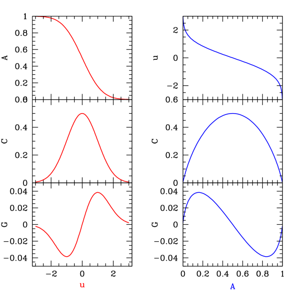
Figure 1: Global Minkowski functionals of a Gaussian field. Three panels on the left hand-side show three global Minkowski functionals: the total fraction of the area in the excursion set, $A$, contour length per unit area, $C$, and genus per unit area, $G$, as a function of the level, $u$. The panels on the right hand-side show (from top to bottom) the level, $u$, contour length, $C$, and genus $G$ as a function of the total area $A$.

where $R=\sqrt{2}/\sigma_{1}$ is the scale of the field; $\sigma_{1}$ is the rms of the first derivatives (in statistically isotropic fields both derivatives $\partial u/\partial x$ and $\partial u/\partial y$ have equal rms). It is assumed that the field is normalized: $<u>=0$ and $<u^{2}>=1$. The Minkowski functionals as functions of the level are shown in the left hand side panels of Fig.1.

The parameterization by the level is useful for many applications. However, for the study of the morphology of the fields and Gaussianity in particular the parameterization by $A$ is much better because it makes the statistics independent of the PF and considerably less correlated with each other [2001].

The total area of the excursion set $A$ of the field was suggested to parameterize other quantities [1996, 2001]. Parameter $A$ is a single valued function of ${\nu}$, the parameter used in the most papers studied genus (Park et al. [2001] and references therein) and therefore every function of ${\nu}$ can be also expressed as a function of $A$. However $A$ is more directly related to the morphology of random fields. In addition, being equal to the cumulative probability function (CPF) it has a very simple statistical and geometrical meaning. Imagine that the excursion set ($u>u_{c}$) is painted black while the rest of the map ($u<u_{c}$) remains white. Then the fraction of the area in black equals $A$. The right hand side panels in Fig.1 show the level, $u$, total contour length, $C$ and genus, $G$ as a function of the total area of the excursion set $A$ for a Gaussian field.

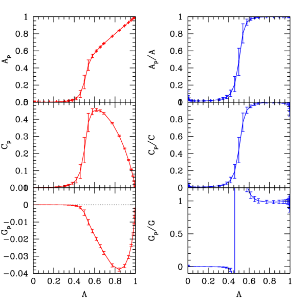
Figure 2: Percolation curves of Gaussian fields. Three panels on the left hand-side show: the area, $A_{p}$, contour length, $C_{p}$ and genus, $G_{p}$ of the largest region as a function of $A$ in the same units as in Fig.1. The right hand side panels show the ratios of the Minkowski functionals of the percolating region to the corresponding global Minkowski functionals . The error bars show $1\sigma$ errors of the Monte Carlo simulations

It has been noticed that percolation properties of the field can be useful for detecting some types of non-Gaussianity [1982, 1983, 1983, 1984, 1993]. The Minkowski functionals of the largest by area region are excellent parameters to characterize the percolation properties of the field. In contrast to the global Minkowski functionals they are not known in an analytic form. Figure 2 shows the Minkowski functionals of the largest region for a Gaussian field obtained from a large ensemble ($N=1000$) of large Monte Carlo simulations ($1024^{2}$ grid).

It should be stressed that the major reason of using $A$ as an independent parameter consists in isolating independent morphological information that is not present in the probability function (PF). For example, $C=C(A)$ carries only PF-independent information, while $C=C(u)$ mixes it up with the information stored in the PF.

4 Examples of Non-Gaussian Fields

It is interesting to compare how some of the n-point functions and morphological characteristics signal the presence of non-Gaussianity in the field. We consider two examples with quadratic and cubic non-Gaussianity. The former has been suggested as a model having plausible physical mechanisms producing small deviations from Gaussianity [1993, 1994, 1994]. The latter has no physical motivations and is taken as a toy model only.

4.1 Cubic Model

First we consider a transformation

$$v=u+\beta u^{3},$$ (5)

where $\beta$ is assumed to be positive, which guarantees monotonicity of the mapping. The parent field $u$ is assumed to be a normalized Gaussian field with $<u>=0$ and $<u^{2}>=1$. The CPF of the resulting field is

$$F(v)=F_{G}(u_{s}),$$ (6)

where $u_{s}$ is the solution of the cubic equation $u_{s}+\beta u_{s}^{3}=v$ . Although the solution could be obtained in a closed form the expression is quite cumbersome therefore we take the limiting case of small $\beta$

$$u_{s}\approx v-\frac{\beta v^{3}}{1+3\beta v^{2}}.$$ (7)

Thus, the CPF becomes

$$F(v)=\frac{1}{2}\left\{1-{\rm erf}\left[\frac{1}{\sqrt{2}}\left(v-\frac{\beta v^{3}}{1+3\beta v^{2}}\right)\right]\right\}$$ (8)

and the PF can be obtained by differentiation: $f(v)=-dF/dv$.

The two- and three-point correlation functions of this field can be easily obtained for an arbitrary $\beta$

$$\xi_{2}(1,2) = (1+6\beta)\xi_{g}(1,2)+3\beta^{2}\xi_{g}(1,2)\left[3+2\xi_{g}^{2}(1,2)\right],$$ (9)

$$\xi_{3}(1,2,3) = 0$$ (10)

where $\xi_{i}(1,2)$ is a shortcut to $\xi_{i}(r_{1},r_{2})$. The function $\xi_{g}$ is the two-point correlation function of the parent field $u$. To the linear order in $\beta$ the two point function remain the same by the form but acquires a different normalization $(1+6\beta)$. The reason why the three point function does not show the presence of non-Gaussianity is the symmetry of the mapping: $u\rightarrow v$ is mapped by an odd function.

Global Minkowski functionals $C(A)$ and $G(A)$ as well as the percolation statistics $A_{p}=A_{p}(A)$, $C_{p}=C_{p}(A)$ and $G_{p}=G_{p}(A)$ remain exactly same as in the parent Gaussian field since the transformation simply relabels the levels without changing the contour lines. However, if they were expressed as functions of the level ($C(v)$ and $G(v)$) they would differ from $C_{G}$ and $G_{G}$ because some non-Gaussian signal leaks into them from the CPF. We will illustrate this point when discuss the quadratic model.

The full information about non-Gaussianity of the field is obviously stored in one number (the value of $\beta$) and can be obtained from one point statistics (the PF or equivalently CPF) however the non-Gaussianity is not detected by the odd order n-point statistics. In a generic case of monotonic mapping $v=\phi(u)$ where $\phi$ is a monotonic but not necessarily odd function of $u$ all n-point functions would detect non-Gaussianity.

4.2 Quadratic Model

As it was mentioned before the quadratic non-Gaussianity is particularly popular in cosmology. The quadratic model is the sum of a Gaussian field and its square

$$v=u+\alpha(u^{2}-1).$$ (11)

In this paper we assume that $u$ is normalized to unity: $<u>=0$ and $<u^{2}>=1$. If one likes a different normalization $<u^{\prime}>=0$ but $<u^{\prime 2}>=\sigma^{\prime 2}$ and the quadratic transformation in the form

$$v^{\prime}=u^{\prime}+\alpha^{\prime}(u^{\prime 2}-\sigma^{\prime 2})$$ (12)

then the relations between the parameters of the two transformations are as follows

$$u^{\prime}=\sigma^{\prime}u,~{}~{}~{}v^{\prime}=\sigma^{\prime}v,~{}~{}~{}\alpha^{\prime}=\alpha/\sigma^{\prime}.$$ (13)

For certainty, without losing generality we will assume $\alpha>0$. Solving eq. 11 for $u$ and denoting the solutions as $u_{1}$ and $u_{2}$ ($u_{2}<u_{1}$) one obtains

$$u_{1}=\frac{\sqrt{1+4\alpha(\alpha+v)}-1}{2\sqrt{2}\alpha},~{}~{}~{}~{}~{}u_{2}=\frac{-\sqrt{1+4\alpha(\alpha+v)}-1}{2\sqrt{2}\alpha}.$$ (14)

The CPF of the field can be written then as

$$F(v) = 1-\frac{1}{2}\left[{\rm erf}\left(\frac{\sqrt{1+4\alpha(\alpha+v)}-1}{2\sqrt{2}\alpha}\right)-{\rm erf}\left(\frac{-\sqrt{1+4\alpha(\alpha+v)}-1}{2\sqrt{2}\alpha}\right)\right].$$ (15)

Differentiating it with respect to $v$ one easily obtains the PF [1993, 2000] :

$$f(v)=\frac{1}{\sqrt{2\pi}}\frac{\exp\left(-\frac{(\sqrt{1+4\alpha(\alpha+v)}-1)^{2}}{8\alpha^{2}}\right)+\exp\left(-\frac{(-\sqrt{1+4\alpha(\alpha+v)}-1)^{2}}{8\alpha^{2}}\right)}{\sqrt{1+4\alpha(\alpha+v)}}.$$ (16)

The PF has a weak singularity at $v=-1/(4\alpha)-\alpha$

$$f(v)\approx\sqrt{\frac{2}{\pi}}\frac{\exp(-\frac{1}{8\alpha^{2}})}{\sqrt{1+4\alpha(\alpha+v)}}.$$ (17)

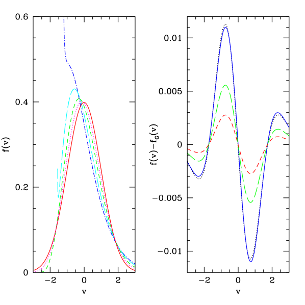
Figure 3: The probability functions in the quadratic model for five amplitudes: ${\alpha}=0.25,0.18,0.1$ and $0.05$ corresponding to the dot-dashed, long dashed, short dashed, and dotted lines are shown in the left hand side panel. The solid line is the Gaussian PF. The difference between the PF of the quadratic model and the Gaussian PF for three amplitudes : ${\alpha}=0.02,0.01$ and $0.005$ corresponding to dotted, long dashed and short dashed lines is shown if the right had side panel. The solid line shows the analytic linear approximation (eq. 18) with the amplitude ${\alpha}=0.02$.

The PF is shown in Fig.3 for a several values of the parameter $\alpha$. The left hand side panel shows the PF for a relatively large amplitudes ${\alpha}=0.25,~{}0.18,~{}0.1,~{}0.05$. For small amplitudes a better illustration is the difference of the PF and Gaussian PF shown in the right hand side panel (${\alpha}=0.02,~{}0.01,~{}0.005$). Note that for small ${\alpha}$

$$f(v)\approx\left[1+{\alpha}h(v)\right]f_{G}(v)$$ (18)

where

$$h(v)=v(v^{2}-3)$$ (19)

and $f_{G}(v)$ is the Gaussian PF. The function $0.02h(v)f_{G}(v)$ is shown by the solid line in the right hand side panel of Fig. 3. It almost merge with the exact PF shown by the dotted line. The agreement is even better for smaller values of ${\alpha}$.

The two and three point functions are respectively

$$\xi_{2}(1,2) = \xi_{g}(1,2)+2\alpha^{2}\xi_{g}^{2}(1,2),$$ (20)

$$\xi_{3}(1,2,3) = 2\alpha\left[\xi_{g}(1,2)\xi_{g}(1,3)+\xi_{g}(1,2)\xi_{g}(2,3)+\xi_{g}(1,3)\xi_{g}(2,3)\right]$$ (21)

$$+ 8\alpha^{3}\xi_{g}(1,2)\xi_{g}(1,3)\xi_{g}(2,3).$$ (22)

In the case of quadratic mapping (11) the three-point function detects non-Gaussianity in the linear order in ${\alpha}$. In this case all even order functions vanish in linear order of $\alpha$ due to symmetry of the mapping.

The global Minkowski functionals of the field can be also readily obtained

$$C(v) = C_{G}\left(\frac{\sqrt{1+4\alpha(\alpha+v)}-1}{2\sqrt{2}\alpha}\right)+C_{G}\left(\frac{-\sqrt{1+4\alpha(\alpha+v)}-1}{2\sqrt{2}\alpha}\right)$$ (23)

$$G(v) = G_{G}\left(\frac{\sqrt{1+4\alpha(\alpha+v)}-1}{2\sqrt{2}\alpha}\right)-G_{G}\left(\frac{-\sqrt{1+4\alpha(\alpha+v)}-1}{2\sqrt{2}\alpha}\right)$$ (24)

where $C_{G}(u)$ and $G_{G}(u)$ are the Gaussian global Minkowski functionals (eq.4). The $\chi^{2}$ field with one degree of freedom is obviously a particular limiting case of this model and has been discussed in great detail [1990, 1994, 1987, 1999, 2000].

Figure 4 (left hand side panels) shows global Minkowski functionals as a function of the level for four values of the amplitude ${\alpha}=0.25,~{}0.18,~{}0.1,~{}0.05$. Combining the equation for the CPF (15) and recalling that $A(v)\equiv F(v)$ one can also plot $C$ and $G$ as functions of $A$ (Fig.4, right hand side panels). The Gaussian curves are shown by solid lines in all panels. One easily sees that the non-Gaussian signature is much stronger in the left hand side panels. This is due to leaking of some non-Gaussian information into the $C(v)$ and $G(v)$ curves from the PF. The curves $C(A)$ and $G(A)$ show only the non-Gaussianity that is absent in PF and therefore show nothing when such information is absent. This is why one can see only two non-Gaussian curves corresponding to ${\alpha}=0.25$ and $0.18$ in the right hand side panels. Although all four non-Gaussian curves are plotted the curves corresponding to ${\alpha}=0.1$ and $0.05$ are merged with the Gaussian curves and are not seen. The curves corresponding to ${\alpha}=0.1$ and $0.05$ are clearly seen in the left hand side panels although, as shown below, the morphology of these fields is practically Gaussian or more exactly the non-Gaussian morphology is completely absent in maps with $N_{pix}<10^{7}$. Another illustration of this effect is provided by the comparison of the $C(v)$ and $G(v)$ curves at $v>1$ with the $C(A)$ and $G(A)$ at $A<0.16$. The mapping (eq. 11) is monotonic and thus does not change the morphology of the field at small amplitudes in this range of $v$ or $A$. All the curves merge in the right hand side panels manifesting the similarity of the morphology to the Gaussian one, but they are clearly distinct in the left hand side panels due to leaking of some non-Gaussianity from the PF.

As a whole the quadratic model (11) is not a monotonic mapping: $v$ is monotonically increasing at at $u>-1/2\alpha$ and monotonically decreasing at $u>-1/2\alpha$. This results in two terms in eq. 15 and eq. 24 as well as in the deviation of the morphology from the Gaussian one because the regions belonging to the excursion set $v>v_{c}$ belong to different excursion sets in the parent field $u$: $S_{1}~{}[u>u_{1}(v_{c})]$ and $S_{2}~{}[u<u_{2}(v_{c})]$ (eq. 14).

Consider now the limiting case of small $\alpha$. For small $\alpha$ the decreasing branch of the mapping is shifted to large negative $u$ and thus greatly reducing the second terms in eq. (16 and 24). Therefore,

$$A(v) \approx \frac{1}{2}\left[1-{\rm erf}\left(\frac{\sqrt{1+4\alpha(\alpha+v)}-1}{2\sqrt{2}\alpha}\right)\right]$$ (25)

$$C(v) \approx C_{G}\left(\frac{\sqrt{1+4\alpha(\alpha+v)}-1}{2\sqrt{2}\alpha}\right)$$ (26)

$$G(v) \approx G_{G}\left(\frac{\sqrt{1+4\alpha(\alpha+v)}-1}{2\sqrt{2}\alpha}\right)$$ (27)

and the mapping becomes almost monotonic.

In cosmology one is usually interested in detecting the possibly smallest non-Gaussianity. For small ${\alpha}$ the quadratic transformation can be practically monotonic for a map of a finite size. Let us consider a map with $N_{pix}$ pixels and calculate the critical value $\alpha_{c}$ corresponding to the value of $\alpha$ when the double valued character of transformation (11) is observed on average at one pixel only. The minimum of the parabola (11) is reached at $u_{min}=-1/2\alpha$. Therefore the probability that a map of the size $N_{pix}$ contains on average one pixel where the monotonicity of (11) is broken is

$$1-F_{G}(u_{min})\equiv 1-F_{G}(-1/2{\alpha}_{c})=\frac{1}{N_{pix}}.$$ (28)

The solution for $N_{pix}$ has a simple analytic form for ${\alpha}_{c}\ll 1$

$$N_{pix}\approx\sqrt{\frac{\pi}{2}}\frac{1}{{\alpha}_{c}}\exp(\frac{1}{8{\alpha}_{c}^{2}}).$$ (29)

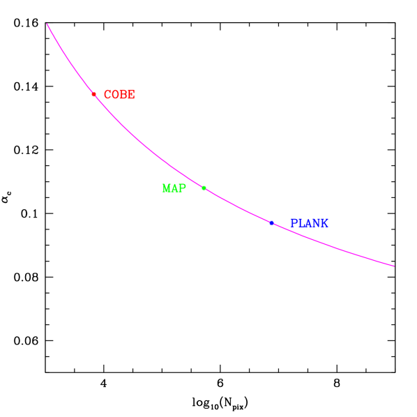
Figure 5: The triviality limit for the quadratic model ${\alpha}_{c}={\alpha}_{c}(N_{pix})$. If the amplitude ${\alpha}<{\alpha}_{c}$ then the quadratic model is fully described by the PF only on a grid of the size $N_{pix}$.

Critical amplitude ${\alpha}_{c}$ is plotted as a function of $\log_{10}(N_{pix})$ in Fig.5 with the points corresponding to the best resolutions of the COBE, MAP and Plank experiments. One easily sees that only relatively large $\alpha$ (roughly ${\alpha}>{\alpha}_{c}\approx 0.09$) may result in the deviation of the quadratic model (11) from monotonicity for even very large maps. It means that the full information about the non-Gaussianity of the quadratic model can be obtained from a one point function only if ${\alpha}<0.09$. Nothing can be gained by applying more complex n-point statistics.

5 Trivial Non-Gaussianity

From the examples of Sec. 4 one can make a further step to a little more general case. Consider a monotonic mapping of a Gaussian field $u\rightarrow v$: $v=\phi(u)$ with $dv/du>0$ (the case with $dv/du<0$ is similar). This transformation obviously affect only the PF

$$F(v)=F_{G}(\phi^{-1}(v))$$ (30)

where $F_{G}$ is the Gaussian cumulative probability function and $\phi^{-1}(v)$ is the inverse of the function $\phi(u)$. The PF can be found by the differentiation of the above expression.

The shapes of the level contours do not change in the resulting field because the contours of constant $v$ coincide with the corresponding contours of constant $u$. The non-Gaussian fields obtained by this kind of mapping can be called trivial since all its non-Gaussianity is described by the one-point function (e.g. PF).

The cubic as well as quadratic model with roughly $\alpha<0.09$ (in maps with $N_{pix}<10^{7}$) are examples of trivial non-Gaussian fields. Another example of a trivial non-Gaussian field is given by the exponential mapping

$$v=\exp(u)$$ (31)

where $u$ is a Gaussian field. The resulting field has the lognormal PF and exactly the Gaussian morphology.

If $v=\phi(u)$ is not a monotonic function then $u=\phi^{-1}(v)$ is a multiple valued function. As a result some regions of the excursion set with $u>u_{c}$ may not satisfy the condition $v(u)>v_{c}(u_{c})$ and vice versa. This case is a little more complex but also can be fully treated analytically in terms of the Minkowski functionals .

One point function PF (or CPF) is in many respects the simplest statistics requiring only $O(N_{pix})$ operations. The other statistics (e.g. n-point correlation functions) share some information with the PF. The morphological statistics (Minkowski functionals ) are easy to isolate from the PF by parameterizing them by the area of the excursion set. We are not aware of the general method of isolation the morphological non-Gaussianity in other non-Gaussian statistics. However, there is a simple technique allowing to assess the sensitivity of any statistics to the morphological non-Gaussianity.

Let us relabel the levels of the field $v\rightarrow u$ according to the equation

$$F(v)=F_{G}(u)$$ (32)

where $F(v)$ and $F_{G}(u)$ are the CPF of the original and Gaussian fields respectively. The new field has the Gaussian PF by design but restores the morphology of the original field because the contour lines have been only relabeled but not distorted. Then computing any non-Gaussian statistics for the new field one can be sure that it depends only on the information that is absent in the PF. For instance, if the original field was trivial non-Gaussian then after this transformation all non-Gaussian statistics must vanish. This transformation of the field can be called the gaussianization of the field. It was used for the purpose of recovery of the primordial fluctuations from the present day galaxy distribution [1992] and recovery of the power spectrum from QSO $Ly\alpha$ forest spectra [1999].

It is worth stressing that the gaussianization neither simply smoothes the original field no re-scales the spectrum as in the transformation suggested by Wu [2001]. It is local but in general highly nonlinear and its only purpose is to isolate non-Gaussian information which is complimentary to the PF [2001]. It certainly affect all n-point functions and n-point spectra including the spectrum of the field. It also changes the phases and therefore may be useful in studies similar to that by Coles & Chiang [2000].

6 The Amplitude of the Quadratic model

Assuming that detecting the possibly smallest non-Gaussianity is the goal we consider a few estimators of the amplitude of the quadratic non-Gaussianity ${\alpha}$ ignoring minute effects on morphology. It means that ${\alpha}$ is to be less than ${\alpha}_{c}$ of eq. 29 (see also Fig. 5). Luo and Schramm (1993) derived the skewness in the quadratic model. To linear approximation in $\alpha$ it is

$$S\equiv\frac{<(v-\bar{v})^{3}>}{\sigma_{v}^{3}}=<v^{3}>\approx 6{\alpha}.$$ (33)

The last equality is because $\bar{v}=0$ and $\sigma_{v}=1$. Thus, measuring the skewness one can estimate the amplitude of the quadratic component. One can also easily obtain the estimates of $\alpha$ from higher central moments

$$c_{5}\approx 60\alpha,~{}~{}~{}~{}c_{7}\approx 630\alpha$$ (34)

where $c_{i}$ are the corresponding central moments $c_{i}=<v^{i}>$ since $<v>=0$ and $<v^{2}>=1$. In principle, any of odd moments can be used for the estimate of the amplitude $\alpha$.

Since the higher moments depend stronger on the tails of the PF one might think that the most accurate is the estimate based on the skewness. As we shall see this trend is very week at least in the case of the lowest three moments (n=3, 5 and 7).

Using the asymptotic form of $f(v)$ (eq. 17) one also can derive ${\alpha}$ using the least square estimator. Suppose there are $N$ measurements of $v$ binned in $N_{b}$ equal bins, $\delta v$, ($n_{i},~{}~{}i=1,\cdots,N_{b}$). Then minimizing the $\chi^{2}$

$$\chi^{2}=\sum\limits_{i=1}^{N_{b}}\left[\frac{n_{i}-n({\alpha},v_{i}))^{2}}{\sigma_{i}}\right]$$ (35)

one can obtain ${\alpha}$. Simple calculations result in

$${\alpha}\approx\left\{\sum\limits_{i=1}^{N_{b}}\frac{\left[n_{i}^{2}-N^{2}f_{G}(v_{i})^{2}\delta v^{2}\right]h(v_{i})}{Nf_{G}(v_{i})\delta v}\right\}\left\{2\sum\limits_{i=1}^{N_{b}}\frac{n_{i}^{2}h^{2}(v_{i})}{Nf_{G}(v_{i})\delta v}\right\}^{-1}.$$ (36)

Considering the propagation of errors one can also estimate the standard deviation of ${\alpha}$

$$\sigma_{{\alpha}}\approx\left\{2\sum\limits_{i=1}^{N_{b}}\frac{n_{i}^{2}h^{2}(v_{i})}{Nf_{G}(v_{i})\delta v}\right\}^{-1/2}.$$ (37)

Assuming $n_{i}\gg 1$ one can simplify eq.37

$$\sigma_{{\alpha}}\approx N^{-1/2}\left(\sum\limits_{i=1}^{N_{b}}f_{G}(v_{i})h^{2}(v_{i})\delta v\right)^{-1/2}\approx N^{-1/2}\left(\int\limits_{-\infty}^{\infty}f_{G}(v)h^{2}(v)dv\right)^{-1/2}=(6N)^{-1/2}.$$ (38)

This can be used for the estimate of the statistical limit on the value of ${\alpha}$ on a grid of size $N_{pix}$. Requiring that $|{\alpha}|>2\sigma_{{\alpha}}$ ($2\sigma$ detection) one obtains

$$|{\alpha}|>(3N_{pix}/2)^{-1/2}.$$ (39)

Thus, for the map of the size of $N_{pix}\sim 10^{6}$ the value ${\alpha}$ must be greater than ${\alpha}_{min}\sim 10^{-3}$ in order to be detected by this method. For an actual CMB experiment eq. 38 is good but still an approximation. The effects of the radiation transfer function are needed to be included in a realistic application to CMB map.

7 Monte Carlo Simulations

In order to check the above analytic calculations and study the other effects we use simple Monte Carlo simulations. First, a Gaussian field $u$ ($<u>=0,<u^{2}>=1$) is generated in a square of the size $N_{pix}=N_{1}\times N_{1}$. We used the flat spectrum smoothed at $k_{s}=N_{1}$ in units of the fundamental wavelength, $P\propto\exp(-k^{2}/k_{s}^{2})$. Then, the field $v=u+{\alpha}(u^{2}-1)$ was obtained and the amplitude ${\alpha}$ was estimated by four methods described above: ${\alpha}_{1}$ from the least square estimator (eq. 36), ${\alpha}_{3}$ from the skewness (eq. 33), and ${\alpha}_{5}$ and ${\alpha}_{7}$ from the fifth and seventh moments respectively (eq. 34).

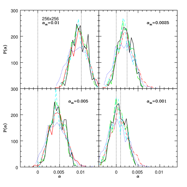
Figure 6: The probability functions of the amplitudes measured in the Monte Carlo simulations of the $256^{2}$ maps. The amplitudes ${\alpha}_{1}$ (obtaind from eq. 36), ${\alpha}_{3}$ (eq. 33), ${\alpha}_{5},{\alpha}_{7}$ (eq. 34) and ${\alpha}_{m}=({\alpha}_{1}+{\alpha}_{3}+{\alpha}_{5}+{\alpha}_{7})/4$ are shown by the dot-dashed, long dashed, short dashed, dotted, and solid lines respectively. The vertical dotted lines mark ${\alpha}=0$ and the model value ${\alpha}_{m}$ in the simulations.

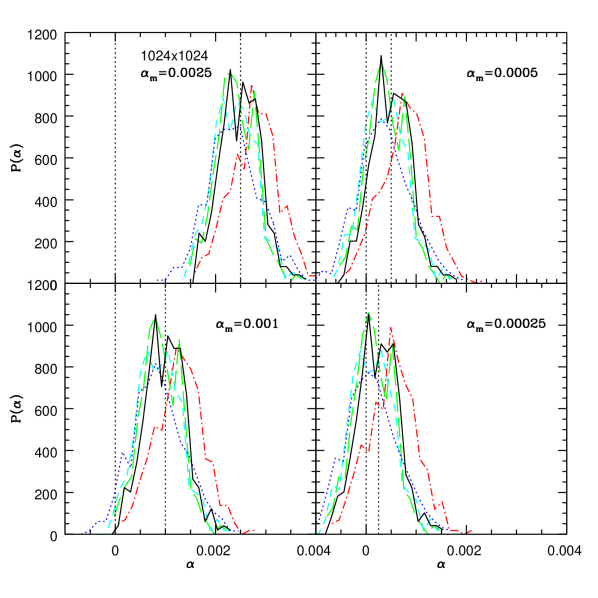
Figure 7: The probability functions of the amplitudes measured in the Monte Carlo simulations of the $1024^{2}$ map. Notations are as in Fig. 6

In addition, the mean of four was also computed: ${\alpha}_{m}=({\alpha}_{1}+{\alpha}_{3}+{\alpha}_{5}+{\alpha}_{7})/4$. Figures 6 and 7 show the probability functions $P({\alpha})$ measured in 400 realizations of the $256^{2}$ and $1024^{2}$ maps. Four panels show results for four different amplitudes illustrating the reliability of the detection of the non-Gaussianity and measurement of the value of ${\alpha}$. Five curves in each panel show the distribution functions $P({\alpha}_{1})$, $P({\alpha}_{3})$, $P({\alpha}_{5})$, $P({\alpha}_{7})$, and $P({\alpha}_{m})$. It is a little surprising that the curves heavily overlap which demonstrates that there is no much difference in the distributions of ${\alpha}$ obtained by different methods although the mean of four is always has a little shorter tails (solid lines) while the estimate based on the highest moment $c_{7}$ often spreads a little wider than others (dotted lines). Although all ${\alpha}_{i}$ are not independent they are the most sensitive to different parts of the PF. The ${\alpha}_{7}$ is obviously sensitive to the higher values of the PF than others and thus is probably the least reliable.

Comparing the theoretical estimates of the statistical limits on the measurement of the quadratic non-Gaussianity (0.003 for the $256^{2}$ and 0.0008 for $1024^{2}$ map eq. 38) with Fig. 6 and 7 we conclude that eq. 38 predicts the errors in measuring ${\alpha}$ quite accurately.

In these simulations the field $v$ obviously has a scale that corresponds roughly to the pixel size. If the scale of the field was below the resolution of the map the field would be smoothed. Smoothing obviously erases non-Gaussianity because of the central limit theorem. We model the resolution effect by smoothing the original non-Gaussian field with the Gaussian filter

$$W(k,k_{sm})=\exp(-\frac{k^{2}}{2k^{2}_{sm}}).$$ (40)

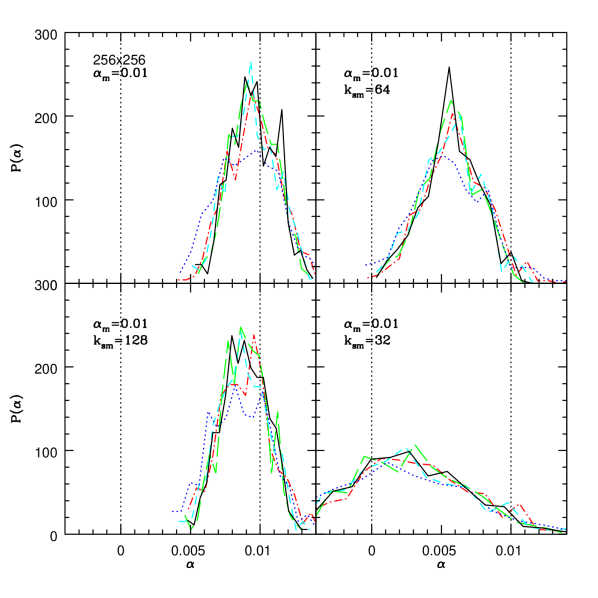
Figure 8: The effect of resolution in the $256^{2}$ maps. Four panels show the PFs of the measured amplitudes when the initial quadratic field was unsmoothed (left top), filtered with the Gaussian window with the Nyquist frequency $k_{sm}=128$ (left bottom), with $k_{sm}=64$ (right top), and with $k_{sm}=32$ (right bottom). Notations are as in Fig. 6

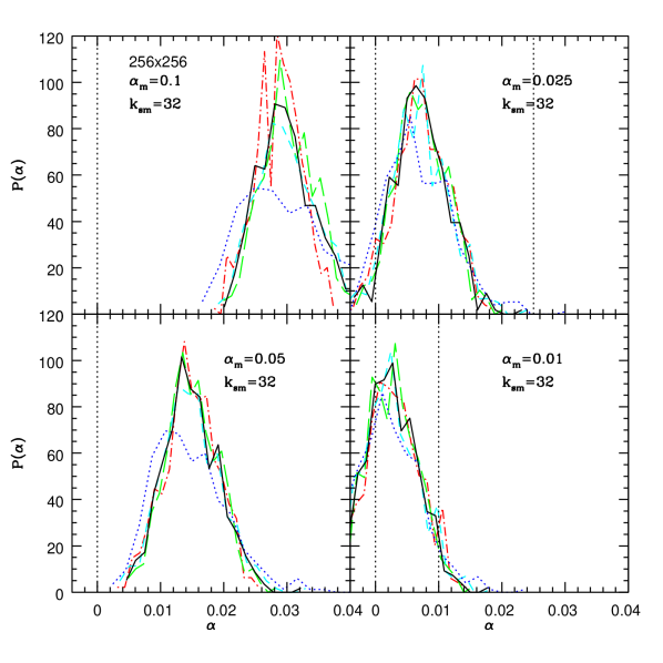
Figure 9: The effect of the amplitude in the $256^{2}$ maps. Four panels show the PFs of the measured amplitudes if the initial quadratic field smoothed with $k_{sm}=32$ had the amplitudes ${\alpha}=0.1$ (left top), ${\alpha}=0.05$ (left bottom), ${\alpha}=0.025$ (right top), and ${\alpha}=0.01$ (right bottom). Notations are as in Fig. 6

Real CMB maps are likely to be smoothed which obviously reduces the ability of measuring $\alpha$. Figure 8 illustrates this effect. The quadratic non-Gaussianity can be easily detected and the amplitude ${\alpha}=0.01$ can be roughly estimated from a $256^{2}$ map if the scale of non-Gaussianity equals the pixel size. In the top left panel the distribution function of $\alpha$ measured in a thousand maps peaks at about right value ${\alpha}=0.01$. The width of the distribution function definitely allows the detection but the accuracy of the measurement is not very high. If it was observed with four times lower resolution corresponding to the smoothing scale $k_{sm}=64$ in the units of the fundamental wavenumber the measured amplitude would be on average a half of the original one. At the resolution 8 times of the original scale of the non-Gaussianity the detection becomes impossible. Of course, this depends on the amplitude. If the amplitude was 2.5 times higher (${\alpha}=0.025$) then the detection of the non-Gaussianity would still possible even at the resolution 8 times of the original scale as illustrated by by the right top panel of Fig. 9 however the measurement of the amplitude would not be possible even it was ten times higher ${\alpha}=0.1$. Generally, smoothing reduces non-Gaussianity and thus makes its measurement more difficult.

8 Summary

The simplest tests for the primordial non-Gaussianity are based on studies of the one-point functions: the PF or CPF and in particular the moments of the PF (skewness, kurtosis, etc. ). However, the Gaussian form of the PF does not guarantee the Gaussianity of the field. The hierarchy of the n-point functions or n-spectra or other tests are supposed to analyze additional information that is not contained in the PF. It is natural to call it morphological information because it is determined by the pattern of the contour lines only.

However, the sensitivity of n-point functions as well as many other statistics to the morphological information is unknown. In fact the n-point functions and other statistics use a great deal of the information stored in the PF. A simple example is provided by the analysis of the quadratic model (eq.11).

At small amplitudes (practically at ${\alpha}<0.1$ ) the field becomes trivial non-Gaussian which means that the full information about the non-Gaussianity is already contained in the PF (eq. 18).

This means that nonzero three-point function if applied to this model (eq. 22) uses exactly same statistical information as the PF. The morphological statistics in the form of the Minkowski functionals of the excursion set ($A$, $C$ and $G$) and percolating region ($A_{p}$, $C_{p}$ and $G_{p}$) obviously recycle the same information as the PF. However, in the last case this information can be easily isolated in $A$ which is the CPF of the field. Other morphological statistics ($C$, $G$ $A_{p}$, $C_{p}$ and $G_{p}$) do not show any non-Gaussian signal if they are expressed as functions of $A$ (Fig. 4). In general, these morphological statistics use the different statistical information than the one-point functions.

Expressing the morphological parameters as functions of $A$ instead of the level $u$ is equivalent to the gaussianization of the field. For other (non morphological) statistics the gaussianization of the field $v$ can be achieved by relabeling the levels of the field $v\rightarrow u$ according to eq. 32. The new field $u$ has the Gaussian PF by design but the geometry and topology of the original field. If any statistic sensitive to non-Gaussianity is applied to the new field $u$ will characterize the geometry and topology of the original field $v$ but free from the effects of the non-Gaussian PF of the original field. Performing this test allows to assess the level of independence of any statistic from the one-point functions.

In line of the above reasoning we showed that the quadratic model results in a trivial non-Gaussian field at small ${\alpha}$. Using this fact we estimated the statistical limit of detecting the quadratic model in the ideal situation when the scale of the field is resolved. This limit is roughly ${\alpha}_{sl}\approx N_{pix}^{-1/2}$ if the parent field $u$ is normalized to unity as in eq. 11 or ${\alpha}^{\prime}_{sl}\sigma^{\prime}\approx N_{pix}^{-1/2}$ if the rms of the parent field is $\sigma^{\prime}$. The Monte Carlo simulations on $256^{2}$ and $1024^{2}$ grids confirm this estimate.

We measured the amplitude of the quadratic non-Gaussianity ${\alpha}$ using four different estimators of ${\alpha}$: ${\alpha}_{1}$ from the least square fitting of the PF (eq. 36) and from three lowest order odd central moments $S=c_{3},c_{5}$ and $c_{7}$

$${\alpha}_{3}=\frac{S}{6},~{}~{}{\alpha}_{5}=\frac{c_{5}}{60},~{}~{}{\alpha}_{7}=\frac{c_{7}}{630}.$$ (41)

In addition, we also computed the mean of the four, ${\alpha}_{m}=({\alpha}_{1}+{\alpha}_{3}+{\alpha}_{5}+{\alpha}_{7})/4$. Quite surprisingly, all four estimators ${\alpha}_{1},{\alpha}_{3},{\alpha}_{5},{\alpha}_{7}$ performed very similarly in all tests. This feature in combination with the Gaussian character of morphological statistics can be used for distinguishing the quadratic non-Gaussianity from other types of non-Gaussianity.

We have illustrated how the resolution and smoothing can affect the detection and measurement of the quadratic non-Gaussianity. In order to be detected the scale of the original non-Gaussian field must be relatively close to the resolution of the map. However, quantifying this effect requires the study of three-dimensional parameter space (the size of the map, $N_{pix}$, the amplitude of the quadratic non-Gaussianity, ${\alpha}$, and the resolution or smoothing scale, $k_{sm}$) and is beyond the scope of this paper.

Acknowledgments: I acknowledge the support of the GRF 2001 and 2002 grants at the University of Kansas. I am grateful to the referee for useful comments and suggestions.

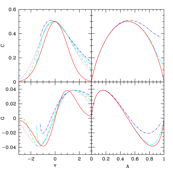
Figure 4: The Global Minkowski functionals $C$ and $G$ for the quadratic model parameterized by the level $v$ are shown in the left hand side panel. the parameterization by the area of the excursion set $A$ is shown in the right hand side panels. The amplitudes are as in the left hand side panel of Fig. 3: ${\alpha}=0.25,0.18,0.1$ and $0.05$ corresponding to the dot-dashed, long dashed, short dashed, and dotted lines. The solid lines show the Gaussian Minkowski functionals .

References

- [ 2001] Aghanim N., Forni O. & Bouchet F.R., 2001, A&A , 365, 341
- [ 1989] Balian R. & Schaeffer R., 1989, A&A , 220, 1
- [ 2000] Banday A.J., Zaroubi S. & Górski K.R., 2000, ApJ , 533, 575
- [ 1983] Bardeen J.M., Steinhardt P.L. & Turner M.S., 1983, Phys. Rev. D, 28, 697
- [ 2000] Barreiro R.b., Hobson M.P., Lasenby A.N., Banday A.J., Górski K.R., & Hinshaw G., 2000, MNRAS , 318, 475
- [ 1998] Bond J.R., Jaffe A.H., 1998, in Proc. XVI Rencontre de Moriond, Microwave Background Anisotropies, ed. F. R. Bouchet (Paris: Editions Fronti res), 197
- [1999] Bromley B. & Tegmark M., 1999, ApJL, 524, L79
- [ 1996] Colley W.N., Gott J.R. & Park, C., 1996, MNRAS , 281, L82
- [ 1988] Coles P., 1988, MNRAS , 234, 509
- [ 1987] Coles P. & Barrow J.D., 1987, MNRAS , 228, 407
- [ 2000] Coles P. & Chiang L-Y., 2000, astro-ph/0010521
- [ 1999] Croft R.A.C., Weinberg, D.H., Pettini M., Hernquist L., & Katz N., 1999, ApJ, 520, 1
- [ 1970] Doroshkevich A.G., 1970, Astrophysics, 6, 320
- [ 1993] Falk T., Rangarajan R. & Srednicki M. 1993, ApJ , ,, 403,L1
- [ 1998] Ferreira P.G., Magueijo J. & Górski K.M., 1998, ApJ , 503, L1
- [ 1994] Gangui A., Lucchin F., Matarrese S., & Mollerach S., 1994, Apj, 430, 447
- [ 1986] Gott III J.R., Melott A.L. & Dickinson M., 1986, ApJ, 306, 341
- [ 1990] Gott III J.R., Park C., Juszkiewicz R., Bies W.E. Bennett D.P., Bouchet R.R., & Stebbins A., 1990, ApJ, 352, 1
- [ 1982] Guth, A.H. & Pi, S.-Y., 1982, Phys. Rev. Lett. , 49, 1110
- [ 1957] Hadwiger H., 1957, Vorlesungen über Inhalt, Oberfläche und Isoperimetrie (Berlin: Springer)
- [ 1982] Hawking A.W., 1982, Phys. Lett. B, 115, 295
- [ 1999] Kerscher M., 1999, astro-ph/9912329
- [ 1993] Klypin A. & Shandarin S.F., 1993, ApJ, 413, 48
- [ 1996] Kogut A., Banday A.J., Górski K.M., Hinshaw G., Smoot G.F., & Wright E.L., 1996, ApJ , 464, L29
- [ 1957] Longuet-Higgins M.S., 1957, Phil. Trans.Roy.Soc.London, A, 249, 321
- [ 1994] Luo X., 1994, ApJ, 427, L71
- [ 1993] Luo X., Schramm D.N., 1993, ApJ, 408, 33
- [ 2000] Magueijo J., 2000, ApJ , 528, L57
- [ 2000] Matarrese S., Verde L. & Jimenez R., 2000, ApJ, 541, 10
- [ 1994] Mecke K.R., Buchert T. & Wagner H., 1994, A&A, 288, 697
- [ 1903] Minkowski H., 1903, Math. Ann., 57, 447
- [ 2000] Mukherjee P., Hobson M.P. & Lasenby A.N., 2000, MNRAS , 318, 1157
- [ 1999] Novikov D.I., Feldman H. & Shandarin S.F., 1999, Int. J.Mod. Phys. D8, 291
- [ 2000] Novikov D., Schmalzing J. & Mukhanov V.F., 2000, astro-ph/0006097
- [ 1998] Pando J., Valls-Gabaud D, Fang L.-Z., 1998, Phys. Rev. Lett. , 81, 4568
- [ 2001] Park C-G., Park C., Ratra B., & Tegmark M., 2001, astro-ph/0102246
- [ 2001] Phillips N.G. & Kogut A., 2001, ApJ , 548, 540
- [ 1999] Schmalzing J., 1999, Ph.D. thesis, Ludwig-Maxmilians-Universität München
- [ 1997] Schmalzing J. & Buchert T., 1997, ApJ, 482, L1
- [ 1998] Schmalzing J. & Górski K.M., 1998, MNRAS, 297, 355
- [ 1983] Shandarin S.F., 1983, Soviet Astron. Lett., 9, 104
- [ 1983] Shandarin S.F. & Zel’dovich Ya.B., 1983, Comments Astrophys. 10, 33
- [ 1984] Shandarin S.F. & Zel’dovich Ya.B., 1984, Phys. Rev. Lett. 52, 1488
- [ 2001] Shandarin S.F., Feldman H.A., Xu Y., & Tegmark M., 2002, ApJS, 141 to be published (astro-ph/0107136)
- [ 1982] Starobinski A.A., 1982, Phys. Lett. B, 117, 175
- [ 2000] Szapudi I., Prunet S., Pogosyan D., Szalay A.S., Bond R., 2000, astro-ph/0010256
- [ 1997] Tegmark M., 1997, Phys. Rev. D, 55, 5895
- [ 1990] Tomita H. 1990, in Formation, Dynamics and Statistics of Patterns, eds. K. Kawasaki, M. Suzuki, & A. Onuki, World Scientific, Singapore, New Jersey, London, Hong Kong, p.113.
- [1997] Turner M.S., 1997, in Generation of Cosmological Large-Scale Structure, eds. D.N. Schramm and P. Galeotti, Kluwer Academic Publishers, Dordrecht/Boston/London, p. 153
- [1994] Vilenkin A. & Shellard P., 1994, Cosmic Strings and other Topological Defects. Cambridge University Press, Cambridge.
- [ 2001] Verde L., 2001, astro-ph/0004341
- [ 2000] Verde L., Wang L., Heavens A.F., & Kamionkowski M., 2000, MNRAS, 313, 141
- [ 2001] Verde L., Jimenez R., Kamionkowski M., & Matarrese S., 2001, astro-ph/0011180
- [ 1994] Worsley K., 1994, Adv. Appl. Prob. 26, 13
- [ 1979] White S.D.M., 1979, MNRAS , 186, 145
- [ 1997] Winitzki S. & Kosowsky A., 1997, New Astronomy, 3, 75
- [ 2001] Wu J-H. P., 2001, astro-ph/0104246
- [2001] Wu J-H. P., Babul A., Borrill J., Ferreira P.G., Hanany S., Jaffe A.H. Lee A.T., Rabii B., Richards P.L., Smoot G.F., Stompor R., & Winant C.D., 2001, astro-ph/0104248
- [ 1996] Yess C. & Shandarin S.F.,1996, ApJ, 465, 2
- [ 1992] Weinberg D.H., 1992, MNRAS, 254, 315
- [ 1982] Zel’dovich Ya. B., 1982, Soviet Astron. Lett., 8, 102