Numerical Methods for the Simulation of Dynamical Mass Transfer in Binaries

Abstract

We describe computational tools that have been developed to simulate dynamical mass transfer in semi-detached, polytropic binaries that are initially executing synchronous rotation upon circular orbits. Initial equilibrium models are generated with a self-consistent field algorithm; models are then evolved in time with a parallel, explicit, Eulerian hydrodynamics code with no assumptions made about the symmetry of the system. Poisson’s equation is solved along with the equations of ideal fluid mechanics to allow us to treat the nonlinear tidal distortion of the components in a fully self-consistent manner. We present results from several standard numerical experiments that have been conducted to assess the general viability and validity of our tools, and from benchmark simulations that follow the evolution of two detached systems through five full orbits (up to approximately 90 stellar dynamical times). These benchmark runs allow us to gauge the level of quantitative accuracy with which simulations of semi-detached systems can be performed using presently available computing resources. We find that we should be able to resolve mass transfer at levels $\dot{M}/{M}>\mathrm{few}\times 10^{-5}$ per orbit through approximately 20 orbits with each orbit taking about 30 hours of computing time on parallel computing platforms.

1 Introduction

Over half of all stars in the sky are actually multiple star systems and, of the binaries, about half again are close enough to one another for mass to be exchanged between the components at some point in their evolution (Trimble, 1983). There is a subset of these close binary systems in which periodic or aperiodic variations in luminosity and spectral features can be explained by on-going mass-transfer events and instabilities in the accretion flow. For example, long term stable mass transfer in which the accretor is either a white dwarf, a neutron star, or a black hole is widely recognized as the mechanism powering cataclysmic variables (Warner, 1995) and X-ray sources (Lewin, van Paradijs & van den Heuvel, 1995). In Algol–type systems an evolved star transfers mass via Roche lobe overflow to a near main–sequence accretor (Batten, 1989; Vesper, Honeycutt & Hunt, 2001). Each of these systems evolves on a (secular) time scale that is long compared to the orbital period of the system, with the mass-transfer rate determined by angular momentum losses from the binary, and thermal relaxation and nuclear evolution of the donor star. In these systems, the fraction of the donor’s mass that is transferred during one orbit is typically $\sim 10^{-12}$ to $10^{-9}$, many orders of magnitude less than what current numerical 3-D hydrocodes can resolve. All of the above systems must have descended from binaries in which the accretor of today was initially the more massive component who evolved first off the main–sequence. The mass transfer in these progenitor systems was in many instances dynamically unstable, yielding mass–transfer rates many orders of magnitude above the currently observed rates and leading in some cases to a common envelope phase (see e.g. Warner 1995; Verbunt & van den Heuvel 1995; Nelson & Eggleton 2001)

In addition, there is a wide class of binary star systems not presently undergoing mass-transfer for which the astrophysical scenarios that have been proposed to explain their origin or ultimate fate involve dynamical or thermal mass-transfer in a close binary, sometimes leading to a common envelope phase of evolution. Examples of such systems are millisecond pulsars (Bhattacharya, 1995), some central stars of planetary nebulae (Iben & Livio, 1993), double degenerate white dwarf binaries, perhaps leading to supernovae of type Ia through a merger (Iben & Tutukov, 1984), or subdwarf sd0, sdB stars (Iben, 1990), and double neutron star binaries, perhaps yielding $\gamma$-ray bursts in a fireball when the neutron stars coalesce (Paczyński, 1986; Ruffert et al, 1997; Mészáros, 2001). The evolutionary scenarios that are drawn upon to explain the existence of some of these systems call for events in which $10\%$ or more of the donor’s mass can be transferred during a single orbit.

If we are to fully understand these rich classes of astrophysically interesting systems — their origin, present evolutionary state, and ultimate fate — it seems clear that we will have to develop numerical algorithms that can accurately simulate mass-transfer events in binary systems under a wide range of physical conditions (for example, systems having a wide range of total masses, mass ratios, and ages) over both short and long evolutionary time scales. The astrophysics community as a whole is far from achieving this ultimate goal, but progress is being made as various groups are methodically tackling small pieces of this very large and imposing problem. Examples of recent progress in the numerical simulation of interacting binaries include two-dimensional simulation of mass transfer in Algol (Blondin, Richards & Malinowski, 1995), three-dimensional evolutions of Roche Lobe overflow in LMC X-4 (Boroson et al, 2001) and the accretion stream in $\beta$ Lyrae (Bisikalo et al, 2000), simulations of the common envelope phase and merger of a point-mass white dwarf with a red giant star (Sandquist et al, 1998), neutron star binary and black hole-neutron star binary mergers in the context of $\gamma$-ray bursts (Janka et al, 1999) and the dispersal of the secondary star’s material in type Ia supernovae (Marietta, Burrows & Fryxell, 2000).

Building on our experience simulating the nonlinear development of dynamical instabilities in self-gravitating systems — such as protostellar gas clouds (Cazes & Tohline, 2000), stellar cores (New, Centrella & Tohline, 2000), and young neutron stars (Lindblom, Tohline & Vallisneri, 2001) — and on our experience in studying mass-transfer in close binaries through analytical and semi-analytical techniques (King et al, 1997; Frank, King & Raine, 2001) we are developing a hydrodynamical tool to study relatively rapid phases of mass-transfer in binary systems. Our immediate aim is to be able to follow the dynamical redistribution of material through $\sim 10-30$ orbits after the onset of a mass-transfer instability, in binary systems having a wide range of initial mass ratios with either star initially selected to be in contact with its Roche lobe and thereby become the “donor”. Our simulation tool treats both stars as self-gravitating fluids; they are embedded in the computational grid in such a way that their internal structures are both fully resolved; and the system as a whole is evolved forward in time through an explicit integration of the standard fluid equations, coupled with the Poisson equation so that the Newtonian gravitational field changes along with the mass distribution in a fully self-consistent way. Initially we will examine structures that can be well-represented by relatively simple barotropic (and adiabatic) equations of state, but this constraint can easily be lifted in the future. We will be restricted to studies of relatively rapid phases of mass-transfer because we are integrating the equations of motion forward in time via an explicit integration scheme.

While this simulation tool will not permit us to model stable flows with low mass-transfer rates — such as the observed flows in CVs and X-ray binaries — it should be capable of a wide range of astrophysical applications including: A determination of the conditions required to become unstable toward dynamical mass-transfer in all kinds of close binaries with normal and degenerate components; the ability to follow dynamical phases of mass transfer through to completion, which may mean a return to stability at a new system mass ratio, the formation of a massive disk or a common envelope with or without rapid mass loss from the system, or a merger of the two objects into one; and an investigation of the steady-state structure of secularly stable binaries. Through such investigations we will be able to place on much firmer footing a variety of theoretical scenarios (as alluded to above) that have been proposed to explain the evolution and fate of close binary systems.

With the commissioning of gravitational wave interferometers such as TAMA, LIGO, and VIRGO, there has been a growing interest in understanding the detailed behavior of, especially, neutron star inspirals and mergers. As has been reviewed by Swesty, Wang and Calder (2000; hereafter SWC), a number of different groups have developed hydrodynamical codes to simulate the late stages of inspiral and merger of such compact objects. Indeed, as has been described by New & Tohline (1997) and reviewed by SWC, an earlier version of our own simulation tool has been used to study the dynamical merger of equal-mass systems in which the stellar components were modeled with polytropic, white dwarf, and neutron star equations of state. Generally speaking, however, the last phase of a neutron star inspiral can be modeled with a hydrodynamical code that is less sensitive to initial conditions and more tolerant of errors in the algorithm that integrates the fluid equations forward in time than a hydrodynamical code that is designed to study more generic mass-transfer events in close binary systems. This is because general relativistic effects will necessarily drive a binary neutron star system to smaller separation, guaranteeing that the system will merge; and, even in the absence of relativistic effects, it appears as though a tidal instability that disrupts one or both stars will be encountered before either fills its Roche lobe and encounters a classic mass-transfer instability (Lai, Rasio & Shapiro, 1994).

Building on the work of New & Tohline (1997), we now have a simulation tool that can hydrodynamically follow the orbital evolution of binary stars with high precision. In developing this tool we have made a number of improvements to the hydrodynamics algorithm that was used in this earlier work only to study the tidal merger problem. We also have implemented a self-consistent-field algorithm that can construct very accurate initial equilibrium models of unequal-mass binaries in circular orbits, have paid special attention to the manner in which initial models are introduced into the hydrodynamics code, and have taken full advantage of continuing improvements in high-performance computers. With this tool in hand, we should be able to accurately model the evolution of a much broader class of close binary systems, specifically, systems in which the components initially have unequal mass and/or radii and in which a mass-transfer instability rather than a tidal instability sets in. With the inclusion of appropriate relativistic corrections, this simulation tool should in principle also be able to simulate the merger of equal or unequal mass neutron star binaries, but our intention is not to focus so narrowly on this particular class of systems.

In §2 of this paper, we collect results from theoretical investigations of the linear stability of mass transfer in close binaries and discuss the approximations that have been required to arrive at these results. In §3 we present the self-consistent field method we use for the construction of initial, equilibrium models. We then describe our implementation of a parallel hydrodynamics code for the solution of the ideal fluid equations and Poisson’s equation for an isolated mass distribution in §4. In §5 we compare results from the hydrodynamics code with known solutions for a set of test problems and in §6 we present the results from the evolution of two benchmark detached binaries. These simulations demonstrate our ability to faithfully represent the forces acting on the fluid and allow us to estimate the mass transfer rate we will be able to resolve and the computational expense required to evolve a given system through an interesting number of orbits. We conclude in §7 by summarizing the limits we have been able to attain at practical simulation resolutions and discuss the future application of the tool set to systems of interest.

2 Theoretical Description of Dynamical Mass Transfer

In this section we will argue that Roche lobe overflow in a binary system approximated by two polytropic components can result in mass transfer on a dynamical time scale for a certain range of polytropic indices. A spherical polytrope with uniform entropy in mechanical equilibrium obeys the following mass radius relation (c.f., Chandrasekhar, 1939),

$$R\propto M^{\frac{1-n}{3-n}},$$ (1)

which implies,

$$\frac{\dot{R}}{R}=\left(\frac{1-n}{3-n}\right)\frac{\dot{M}}{M}\equiv\xi_{\mathrm{S}}\frac{\dot{M}}{M}.$$ (2)

Hence, the body will expand upon mass loss for polytropic indices satisfying $1<n<3$.

Consider Paczyński’s (1971) approximation for the effective Roche lobe radius $R^{\mathrm{RL}}_{2}$ of a donor star, taken to be the secondary, with mass $M_{2}$ in a point mass binary of total mass $M$ and separation $a$,

$$\frac{R^{\mathrm{RL}}_{2}}{a}=0.462\left(\frac{M_{2}}{M}\right)^{\frac{1}{3}}.$$ (3)

From this, one obtains the following relation for the logarithmic change in the donor’s Roche lobe radius,

$$\frac{\dot{R}^{\mathrm{RL}}_{2}}{R^{\mathrm{RL}}_{2}}=\frac{\dot{a}}{a}+\frac{1}{3}\frac{\dot{M}_{2}}{M_{2}}-\frac{1}{3}\frac{\dot{M}}{M}.$$ (4)

Upon eliminating the separation in favor of the system’s orbital angular momentum $J$, one arrives at

$$\frac{\dot{R}^{\mathrm{RL}}_{2}}{R^{\mathrm{RL}}_{2}}=2\frac{\dot{J}}{J}-\frac{5}{3}\frac{\dot{M}_{2}}{M_{2}}+\frac{2}{3}\frac{\dot{M}}{M}-2\frac{\dot{M}_{1}}{M_{1}},$$ (5)

where $M_{1}$ is the mass of the accreting star, taken to be the primary. If we further assume that the mass transfer is conservative with respect to the total mass and orbital angular momentum we deduce that,

$$\frac{\dot{R}^{\mathrm{RL}}_{2}}{R^{\mathrm{RL}}_{2}}=\left(2\frac{M_{2}}{M_{1}}-\frac{5}{3}\right)\frac{\dot{M}_{2}}{M_{2}}\equiv\xi_{\mathrm{R}}\frac{\dot{M}_{2}}{M_{2}}.$$ (6)

Comparing equation (2) with equation (6), the condition for stable mass transfer, $\dot{R}_{2}\leq\dot{R}^{\mathrm{RL}}_{2}$ can be expressed as,

$$\xi_{\mathrm{S}}-\xi_{\mathrm{R}}>0,$$ (7)

which, for a given polytropic index, implies a stable mass ratio

$$q\equiv\frac{M_{2}}{M_{1}}=q_{\mathrm{stable}}\equiv\frac{9-4n}{3\left(3-n\right)}.$$ (8)

For a polytropic binary with $n=3/2$ and mass ratio $q>q_{\mathrm{stable}}=2/3$, mass transfer must occur on a dynamical time scale as the donor will readjust its structure within a few sound crossing times to its new mass. Note that if the donor is initially the less massive star (i.e.  $q<1$), the binary separation is expected to steadily increase during the mass transfer event. But, if the donor is initially the more massive component (i.e.  $q>1$), conservation of orbital angular momentum implies that the separation must decrease and that the donor’s Roche lobe radius will contract thus increasing the degree of overflow. The resulting mass transfer rate is expected in this case to be quite substantial.

The dependence of the mass transfer rate on the degree of over-contact can be estimated from the product of the volume swept out by the flow near the inner Lagrange point, $L_{\mathrm{1}}$, in unit time and the local value of the density. The cross section of the flow near $L_{\mathrm{1}}$ will scale as the square of the local sound speed, and the flow velocity is approximately equal to the sound speed. The volume of material transferred in unit time then scales as the cube of the sound speed. The density near the edge of a spherical polytrope of index $n$, radius $R_{2}$, mass $M_{2}$, and polytropic constant $\kappa$ can be found by integrating the equation of hydrostatic equilibrium to obtain,

$$\rho\left(r\right)\approx\left[\frac{GM_{2}}{\kappa\left(n+1\right)}\frac{\left(R_{2}-r\right)}{R^{2}_{2}}\right]^{n}.$$ (9)

If we change variables to $\Delta R_{2}\equiv R_{2}-r$, the width of a spherical shell near the edge of the star, we obtain

$$\rho\left(\Delta R_{2}\right)\propto\left(\Delta R_{2}\right)^{n}.$$ (10)

The sound speed, $c$ in turn obeys,

$$c\propto\rho^{\frac{1}{2n}},$$ (11)

so that

$$\frac{dM_{2}}{dt}\propto\rho^{1+\frac{3}{2n}}\propto\left(\Delta R_{2}\right)^{n+\frac{3}{2}}.$$ (12)

Taking the radius, $r$, to be the effective Roche lobe radius of the donor, $\Delta R_{2}$ is the degree of over-contact. The mass transfer rate is then expected to scale with the degree of over-contact as

$$\frac{dM_{2}}{dt}\propto\frac{M_{2}}{P}\left(\frac{\Delta R_{2}}{R_{2}}\right)^{n+\frac{3}{2}},$$ (13)

where $P$ is the orbital period. This agrees with the calculation of Jedrzjec as presented in Paczyński and Sienkiewicz (1972). For a polytropic index of $n=3/2$, eq. (13) indicates that the mass transfer rate will scale as the cube of the degree of over-contact. While the actual mass transfer rate observed in a fully self-consistent, three-dimensional evolution may differ substantially from the estimate given in (13), it nevertheless indicates that for unstable binaries mass-transfer events will evolve on a dynamical time scale once the donor reaches contact with its Roche lobe.

All the results presented in this section have relied on a great many simplifying assumptions including the disregard of internal angular momentum (spin) in each star, the use of the Roche model, neglecting the intrinsically nonspherical geometry of the components, and assuming that the mass transfer event is, in fact, conservative. To proceed beyond this point one must deal with extended distributions for the density and velocity in some approximation. We would argue further that it is advantageous to use a potential derived from the matter distribution in a self-consistent manner. With these additional complications, the task is well beyond the regime of analytical mechanics, but is tractable if we employ three-dimensional computational fluid dynamical techniques. To investigate short time-scale mass transfer events numerically, we have developed a set of tools for both constructing equilibrium polytropic binaries and a hydrodynamics code to evolve systems of interest in time. These tools are described below.

3 Construction of Equilibrium Models

The iterative method that we have used to generate equilibrium, polytropic binaries is very closely related to the self-consistent field (SCF) technique developed by Hachisu (1986; see also Hachisu, Eriguchi & Nomoto 1986). This technique previously has been used to construct initial models of equal-mass binary systems for dynamical studies of the binary merger problem (see New & Tohline 1997 and SWC). Here we employ a more generalized version of the technique to construct unequal-mass binaries. In the following discussion we use $\mathbf{r}$ to refer to an arbitrary point in space. The vector $\mathbf{R}$ is the cylindrical radius vector which can be expressed as $\mathbf{R}=x\,\hat{\mathbf{x}}+y\,\hat{\mathbf{y}}$. The axis of rotation is always taken to be parallel to, but not necessarily coincident with, the $z$-axis.

The numerical results presented here are in a system of units where the gravitational constant, the radial extent of our numerical grid and the maximum density of one binary component are all taken to be unity. As we are treating polytropic models exclusively in the present work, these models can be scaled to represent different physical systems by choosing a total system mass or orbital separation for example. We would like to emphasize that the polytropic models could represent binaries consisting of neutron stars, white dwarfs or normal stellar components.

Assuming synchronous rotation so that the bodies are stationary in a corotating reference frame, the equations of hydrostatic equilibrium reduce to the following single vector equation,

$$\mathbf{\nabla}\left(H+\Phi-\frac{1}{2}\Omega^{2}\left|\mathbf{R}-\mathbf{R}_{\mathrm{com}}\right|^{2}\right)=0.$$ (14)

Here $\Phi$ is the gravitational potential, $\Omega$ is the angular velocity of the reference frame in which the fluid is stationary, H is the enthalpy, and $\mathbf{R}_{\mathrm{com}}$ is the cylindrical radius vector of the system’s center of mass so that $\left|\mathbf{R}-\mathbf{R}_{\mathrm{com}}\right|$ is each fluid element’s distance from the axis of rotation. For a polytrope of index $n$, $H$ is given to within an arbitrary constant by

$$H=\int\frac{dp}{\rho}=\left(n+1\right)\frac{p}{\rho}=\left(n+1\right)\kappa\rho^{\frac{1}{n}},$$ (15)

where $p$ and $\rho$ are the pressure and density of the fluid, respectively. Equation (14) in turn implies that,

$$H+\Phi-\frac{1}{2}\Omega^{2}\left|\mathbf{R}-\mathbf{R}_{\mathrm{com}}\right|^{2}=C,$$ (16)

for some constant $C$, which in general will be different for each binary component. Hereafter we denote these two integration constants as $C_{\mathrm{1}}$ and $C_{\mathrm{2}}$.

Using equation (16) one can construct an iterative scheme as follows. An initial guess at the density field is constructed. Poisson’s equation is solved to obtain the gravitational potential arising from the chosen mass distribution. This is, by far, the most computationally intensive part of the algorithm. For our work, we have chosen a cylindrical coordinate grid and utilized subroutines from the FISHPACK Fortran subroutine set for the solution of elliptic partial differential equations (Schwarztrauber & Sweet, 1975; Schwarztrauber et al, 2001) with the boundary potential being calculated via a spherical harmonic expansion of the density field utilizing harmonic moments through $\ell=10$.

With the gravitational potential in hand we can use algebraic relations at three boundary points where the density field is forced to vanish in order to set the integration constants $C_{\mathrm{1}}$ and $C_{\mathrm{2}}$, and the value of the angular velocity $\Omega$. The boundary points all lie along the line of centers. They correspond to the inner and outer boundary points for one star, and the inner boundary point for the companion as illustrated in Fig.  1. The values of the gravitational potential at the three boundary points, $\mathbf{r}_{\mathrm{A}}$, $\mathbf{r}_{\mathrm{B}}$ and $\mathbf{r}_{\mathrm{C}}$ are used to solve for the set of constants $\Omega$, $C_{1}$ and $C_{2}$ as follows:

$$\Omega^{2}=\frac{\Phi\left(\mathbf{r}_{\mathrm{A}}\right)-\Phi\left(\mathbf{r}_{\mathrm{B}}\right)}{\frac{1}{2}\left(\left|\mathbf{R}_{\mathrm{A}}-\mathbf{R}_{\mathrm{com}}\right|^{2}-\left|\mathbf{R}_{\mathrm{B}}-\mathbf{R}_{\mathrm{com}}\right|^{2}\right)},$$ (17)

$$C_{1}=\Phi\left(\mathbf{r}_{\mathrm{B}}\right)-\frac{1}{2}\Omega^{2}\left|\mathbf{R}_{\mathrm{B}}-\mathbf{R}_{\mathrm{com}}\right|^{2},$$ (18)

$$C_{2}=\Phi\left(\mathbf{r}_{\mathrm{C}}\right)-\frac{1}{2}\Omega^{2}\left|\mathbf{R}_{\mathrm{C}}-\mathbf{R}_{\mathrm{com}}\right|^{2}.$$ (19)

Equation (16) can then be used to construct the enthalpy throughout the computational domain and, from it, an improved density distribution can be constructed using the relation,

$$\rho=\left\{\begin{array}[]{lr}\rho_{\mathrm{max},i}\left(\frac{H}{H_{\mathrm{max},i}}\right)^{n}&H>0\\ 0&\mathrm{otherwise}\\ \end{array}\right.,$$ (20)

where $i=1,2$ labels the two stellar components. As Hachisu (1986) has explained, it is best to hold the values of $\rho_{\mathrm{max},1}$ and $\rho_{\mathrm{max},2}$ fixed throughout the iteration cycles.

Figure 1: Position of the three boundary points in the equatorial plane for a SCF binary model. At the three boundary points (denoted by asterisks and labeled A, B, and C) the density is forced to vanish. The contours represent density levels for the converged model.

The iteration cycle is then repeated using the improved density distribution until the relative change from iteration to iteration in $C_{\mathrm{1}}$, $C_{\mathrm{2}}$, $\Omega$, and $H_{\mathrm{max},i}$ are all smaller than some prescribed convergence criterion, $\delta$. For a grid resolution of 128 radial points by 128 vertical points by 256 points in azimuth, we typically use a tolerance $\delta=1\times 10^{-4}$.

Unfortunately the self-consistent field method does not allow one to specify physically meaningful parameters such as the binary mass ratio or separation a priori. Instead, as already described, it is best to specify the three boundary points and the maximum density for each body. Nevertheless, the method described above remains, to our knowledge, the most effective means of generating fully self-consistent models of synchronously rotating, equilibrium binary systems with unequal masses and/or radii.

We gauge the quality of a converged solution by the degree to which it satisfies the scalar virial equation. Specifically, we define the following dimensionless virial error

$$\mathrm{VE}\equiv\frac{\left(2K+W+3\Pi\right)}{\left|W\right|},$$ (21)

where the terms appearing in equation (21) are defined by the following integral quantities:

$$K\equiv\frac{1}{2}\int\rho\,\mathbf{v}\cdot\mathbf{v}\,dV,$$ (22)

$$W\equiv\int\rho\,\Phi\,dV,$$ (23)

$$\Pi\equiv\int p\,dV,$$ (24)

where $\mathbf{v}$ is the velocity field as measured in the inertial frame of reference. As applied in the SCF technique, the velocity is entirely due to the rotation of the frame, that is

$$\mathbf{v}=\mathbf{\Omega}\times\left(\mathbf{R}-\mathbf{R}_{com}\right).$$ (25)

In Fig.  2 we plot density contours in the meridional plane for one contact binary system, three semi-detached systems, and two detached systems that we have constructed using the SCF technique. The more massive component always appears on the left of the plots. Figure 3 shows contours in the equatorial plane for the same six systems. The solid lines are at mass density levels of $10^{-5}$, $10^{-4}$, $10^{-3}$, $10^{-2}$ and $10^{-1}$, where the density has been normalized to the maximum density for each model, and the dashed line follows the self-consistently determined critical Roche surface for the system. The binaries all have a polytropic index $n=3/2$; other key parameters for these models are listed in Table 1. Throughout this work we take the secondary component (denoted by a ‘2’) to be the component closest to contact (closest to being the donor). The values of $q=M_{2}/M_{1}$ shown in Table 1 (as well as in Figs. 2 and 3) give the ratio of the mass of the secondary to the primary; the stellar radii ($R_{1}$ and $R_{2}$) and Roche lobe radii ($R^{\mathrm{RL}}_{1}$ and $R^{\mathrm{RL}}_{2}$) have all been normalized to the orbital separation. The stellar radii and Roche lobe radii are the radii of spheres that have a volume equal to the star or critical Roche surface, respectively. For Model 4, the Roche lobe of the primary extends beyond the computational grid so the effective radius of its Roche lobe is only a lower limit. All six of these models were constructed on a cylindrical grid of 128 radial and vertical zones by 256 azimuthal zones.

Table 1: Initial Equilibrium Binary Models

Model	$q$	$\rho_{1}^{\mathrm{max}}$	$R_{1}$	$R^{\mathrm{RL}}_{1}$	$\rho_{2}^{\mathrm{max}}$	$R_{2}$	$R^{\mathrm{RL}}_{2}$	VE
1	1.0000	1.00	0.3720	0.3723	1.00	0.3720	0.3723	$1.5\times 10^{-4}$
2	1.2111	1.00	0.3056	0.3580	0.60	0.3893	0.3915	$1.4\times 10^{-4}$
3	0.4801	1.20	0.3727	0.4401	1.00	0.3126	0.3129	$3.4\times 10^{-4}$
4	0.1999	1.00	0.3817	$>$ 0.5194	0.77	0.2476	0.2478	$2.8\times 10^{-4}$
5 (EB)	1.0000	1.00	0.2984	0.3778	1.00	0.2984	0.3778	$2.0\times 10^{-4}$
6 (UB)	0.8436	1.20	0.3180	0.3919	1.00	0.3200	0.3620	$2.2\times 10^{-4}$

Figure 2: Slice through the meridional plane for six example SCF binaries. Detailed parameters for these models are provided in Table 1. The solid contours are in the logarithm of the normalized density at levels of $10^{-5}$, $10^{-4}$, $10^{-3}$, $10^{-2}$, and $10^{-1}$. The dashed curve traces the critical surface for the self-consistent Roche potential. The density of the stellar components falls rapidly near the surface and on the scale used for these figures, the lowest two contours of the density coincide with one another.

Figure 3: Slice through the equatorial plane for the same six binaries shown in Fig.  2. The solid contours are in the logarithm of the normalized density at levels of $10^{-5}$, $10^{-4}$, $10^{-3}$, $10^{-2}$ and $10^{-1}$. The dashed curve traces the critical surface for the self-consistent Roche potential.

Table 2 lists the resulting virial error for the contact system (Model 1 from Table 1) constructed on grids of differing resolutions. As the convergence criterion, $\delta$, is decreased, the number of required iterations increases. For fixed resolution, the overall quality of the solution does not significantly improve beyond some limiting value of $\delta$, regardless of the number of iterations taken. As the resolution is increased, the virial error decreases roughly in proportion to the square root of the number of grid points.

Table 2: Convergence for SCF Method

R	z	$\phi$	$\delta$	VE
64	64	128	$1.0\times 10^{-3}$	$1.0\times 10^{-3}$
			$1.0\times 10^{-4}$	$6.0\times 10^{-4}$
			$1.0\times 10^{-5}$	$5.5\times 10^{-4}$
			$1.0\times 10^{-6}$	$5.5\times 10^{-4}$
128	128	256	$1.0\times 10^{-3}$	$6.9\times 10^{-4}$
			$1.0\times 10^{-4}$	$2.0\times 10^{-4}$
			$1.0\times 10^{-5}$	$1.5\times 10^{-4}$
			$1.0\times 10^{-6}$	$1.4\times 10^{-4}$
256	256	512	$1.0\times 10^{-3}$	$6.3\times 10^{-4}$
			$1.0\times 10^{-4}$	$1.0\times 10^{-4}$
			$1.0\times 10^{-5}$	$5.2\times 10^{-5}$
			$1.0\times 10^{-6}$	$4.7\times 10^{-5}$
			$1.0\times 10^{-7}$	$4.7\times 10^{-5}$

Due to the symmetry of these initial models about the equatorial plane, we only calculate the models in the half space of $z\geq 0$. Assuming the line of centers coincides with the $x$ axis, the tidal distortion of each star also is symmetric about the $y=0$ plane. Hence, further computational efficiency could be obtained with this technique by limiting the computational grid to only extend from 0 to $\pi$ in azimuth. To date, we have not enforced this additional symmetry constraint, although in practice the converged models display this symmetry.

The SCF method is insensitive to the functional form for the initial guess of the density distribution. For uniform spheres and spherically symmetric Gaussian density distributions one can obtain the same converged model to machine accuracy. We also note that we have found that more rapid convergence for models with soft equations of state (e.g., $n\geq 3/2$) can be achieved by using an even mixture of the current and previous potentials during the iteration. For more rigid equations of state, where there is more mass at the boundary points and hence a greater coupling between the solution near the boundary points and the global solution, such mixing is not necessary and the solution converges rapidly.

4 Hydrodynamics Implementation

4.1 Continuum Mechanics Formalism

We have developed an explicit, conservative, finite-volume, Eulerian hydrodynamics code that is second-order accurate in both time and space to evolve the equilibrium binaries. The program is similar to the ZEUS code developed by Stone & Norman (1992). The integration scheme is designed to evolve five primary variables that are densities of conserved quantities: the mass density, $\rho$, the angular momentum density, $A$, the radial momentum density, $S$, the vertical momentum density, $T$, and an entropy tracer, $\tau$. The entropy tracer,

$$\tau\equiv\left(\epsilon\rho\right)^{\frac{1}{\gamma}},$$ (26)

where $\epsilon$ is the internal energy per unit mass and $\gamma$ is the selected ratio of specific heats of the gas. It is related to the entropy of the fluid through the relation,

$$s=c_{\mathrm{p}}\ln{\frac{\tau}{\rho}},$$ (27)

where $c_{\mathrm{p}}$ is the specific heat at constant pressure. Using the entropy tracer in lieu of the internal energy per unit mass or the total energy density allows us to avoid the finite difference representation of the divergence of the velocity field that must otherwise be used to express the work done by pressure on the fluid.

For the evolutions presented in this paper we have set $\gamma=1+1/n$. We note, however, that by allowing the compressible fluid system to evolve with an adiabatic exponent that differs from this value, the stars will not be homentropic. For example, by selecting an appropriate value of $\gamma>1+1/n$ we can effectively model stars that are convectively stable and that obey a mass-radius relation quite different from the normal polytropic one specified by eq. (2), that is, different from $\xi_{\mathrm{S}}=(1-n)/(3-n)$. By doing this, we expect to be able to closely approximate the mass-radius relationship of main sequence stars. A more detailed discussion of this idea is beyond the scope of this paper.

The set of differential equations that we solve is based on the conservation laws for these five conserved densities. Mass conservation is governed by the continuity equation,

$$\frac{\partial\rho}{\partial t}+\mathbf{\nabla}\cdot\left(\rho\,\mathbf{v}\right)=0,$$ (28)

where $\mathbf{v}$ is the velocity field. The velocity vector is expressed in terms of its components in a cylindrical coordinate system as $\mathbf{v}=u\,\hat{\mathbf{e}}_{R}+v\,\hat{\mathbf{e}}_{\phi}+w\,\hat{\mathbf{e}}_{z}$. The three components of Euler’s equation govern changes in the momentum densities. We express these equations in a frame of reference rotating with a constant angular velocity, $\Omega$, as follows:

$$\frac{\partial S}{\partial t}+\mathbf{\nabla}\cdot\left(S\mathbf{v}\right)=-\rho\frac{\partial\Phi^{\mathrm{eff}}}{\partial R}+\frac{A^{2}}{\rho R^{3}}+2\Omega\frac{A}{R},$$ (29)

$$\frac{\partial T}{\partial t}+\mathbf{\nabla}\cdot\left(T\mathbf{v}\right)=-\rho\frac{\partial\Phi^{\mathrm{eff}}}{\partial z},$$ (30)

$$\frac{\partial A}{\partial t}+\mathbf{\nabla}\cdot\left(A\mathbf{v}\right)=-\rho\frac{\partial\Phi^{\mathrm{eff}}}{\partial\phi}-2\Omega SR,$$ (31)

where,

$$\Phi^{\mathrm{eff}}\equiv H+\Phi-\frac{1}{2}\Omega^{2}R^{2}.$$ (32)

The second and third terms appearing on the right-hand side of eq. (29) represent the curvature of cylindrical coordinates and the radial component of the Coriolis force, respectively. Likewise, the last term appearing on the right-hand side of eq.  (31) represents the azimuthal component of the Coriolis force.

From the first law of thermodynamics we know that in the most general case, the entropy tracer obeys the expression,

$$\frac{\partial\tau}{\partial t}+\mathbf{\nabla}\cdot\left(\tau\mathbf{v}\right)=\frac{\tau}{c_{\mathrm{p}}}\frac{ds}{dt}.$$ (33)

Here we will be considering only adiabatic flows, in which case $ds/dt=0$, so the entropy tracer obeys an advection equation of precisely the same form as the continuity equation, namely,

$$\frac{\partial\tau}{\partial t}+\mathbf{\nabla}\cdot\left(\tau\mathbf{v}\right)=0.$$ (34)

Even though we are performing adiabatic evolutions we can not simply use an adiabatic equation of state ($p=\kappa\rho^{\gamma}$) and disregard the first law of thermodynamics because the polytropic constant is, in general, different for each binary component.

Finally, we solve Poisson’s equation once every integration timestep in order to calculate the force of gravity arising from the instantaneous mass distribution,

$$\nabla^{2}\Phi=4\pi G\rho;$$ (35)

and we use the ideal gas law as the equation of state to close the system of equations, namely,

$$p=\left(\gamma-1\right)\tau^{\gamma}=\left(\gamma-1\right)\rho\epsilon.$$ (36)

It may be argued that our treatment of the thermodynamics of the system as the purely adiabatic flow of an ideal fluid is overly simplified. However, we believe that the self-consistent treatment of both binary components in the presence of the full nonlinear tidal forces is sufficiently complex and novel to warrant the use of a simple equation of state at the present time. This will allow us to establish the qualitative behavior of systems in this limiting case before additional complications leading to nonadiabatic heat transport are introduced into the simulations.

4.2 Finite Volume Representation

Before proceeding with the discussion of the hydrodynamics algorithm that we have implemented to solve the equations presented in §4.1 we first describe the discretization that has been used to represent the exact partial differential equations when they are expressed as approximate algebraic relations between discrete points in the computational grid. As in the ZEUS code, all scalar variables and the diagonal components of tensors are defined at cell centers. The components of vectors are defined at the corresponding faces of the cell. A volume element and the relative positions of the variables within each cell is illustrated in Fig. 4. The cell extends from $R_{i}$ to $R_{i+1}$ in radius, from $z_{j}$ to $z_{j+1}$ in the vertical coordinate, and from $\phi_{k}$ to $\phi_{k+1}$ in the azimuthal coordinate. We represent the staggered variables in the computational mesh with a half-index notation; the coordinates of the center of a grid cell are given by $R_{i+1/2}$, $z_{j+1/2}$, $\phi_{k+1/2}$, for example. A complete listing of the variables and their centering is given in Table 3.

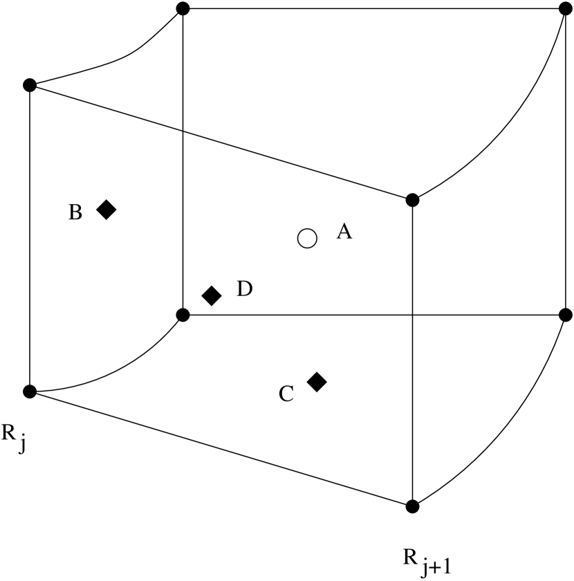
Figure 4: Volume element for a cell-centered quantity (defined at the open circle labeled A) in our cylindrical coordinate mesh. Radial, vertical and azimuthal face-centered quantities are defined at points B, C, and D, respectively. Table 3 lists all of the variables used in the hydrodynamics code along with their centering according to this diagram.

Table 3: Hydrodynamic Variables and their Centering

Centering	Variable	Description
A	$R_{i+1/2}$	Cylindrical Radius Coordinate
	$z_{j+1/2}$	Vertical Coordinate
	$\phi_{k+1/2}$	Azimuthal Coordinate
	$\rho_{i+1/2,j+1/2,k+1/2}$	Mass Density
	$\tau_{i+1/2,j+1/2,k+1/2}$	Entropy Tracer
	$p_{i+1/2,j+1/2,k+1/2}$	Pressure
	$H_{i+1/2,j+1/2,k+1/2}$	Enthalpy
	$\Phi_{i+1/2,j+1/2,k+1/2}$	Gravitational Potential
	$Q^{ll}_{i+1/2,j+1/2,k+1/2}$	Diagonal Components of Artificial Viscosity
B	$S_{i,j+1/2,k+1/2}$	Radial Momentum Density
	$u_{i,j+1/2,k+1/2}$	Radial Velocity
C	$T_{i+1/2,j,k+1/2}$	Vertical Momentum Density
	$w_{i+1/2,j,k+1/2}$	Vertical Velocity
D	$A_{i+1/2,j+1/2,k}$	Angular Momentum Density
	$v_{i+1/2,j+1/2,k}$	Azimuthal Velocity

4.3 Treatment of Advection Terms

Through the method of operator splitting, one can construct a numerical scheme that groups terms of the same physical character together. Again, following along the lines of the ZEUS code we implement a splitting scheme that separates updates of the fluid state due to Eulerian transport (advection) from updates due to the source terms. In this section we describe our treatment of the advection terms.

Given the density $\lambda$ of any conserved quantity $\Lambda$ that satisfies a generic conservation law of the form,

$$\frac{\partial\lambda}{\partial t}+\mathbf{\nabla}\cdot\left(\lambda\,\mathbf{v}\right)=0,$$ (37)

we can replace the differential equation (37) with an equivalent integral equation,

$$\frac{\partial}{\partial t}\int_{V}\lambda\,dV=-\int_{V}\mathbf{\nabla}\cdot\left(\lambda\,\mathbf{v}\right)dV=-\int_{S\left(V\right)}\lambda\,\mathbf{v}\cdot\mathbf{dS}.$$ (38)

Equation (38) must hold for any volume. In particular, it must hold for every volume element within the computational grid. The exact integral relation is then expressible in the following finite volume form for each grid cell:

$$\frac{\lambda^{\left(n+\mathrm{advection}\right)}-\lambda^{\left(n\right)}}{\Delta t}=-\frac{1}{\Delta V}\sum_{i=1}^{6}\lambda_{i}^{\ast}\mathbf{v}\cdot\mathbf{\Delta S_{i}},$$ (39)

where the summation is over all six faces on the surface of the three-dimensional cell. The surface elements, $\mathbf{\Delta S_{i}}$, are naturally face-centered with respect to the control volume in question, so averages must be taken to obtain the advection velocity components necessary to perform the dot product for the momentum densities as shown in eq. (39). We use second-order accurate, linear averages to construct the advection velocities in this case. The amount of $\Lambda$ advected through each face is given by an upwind biased, linear interpolation of the distribution of $\lambda$ to give $\lambda^{\ast}$ as described by van Leer (1979). By construction, the amount of $\Lambda$ that is transported out of one cell immediately flows into the neighboring cell; thus ensuring the conservative nature of the advection scheme.

Unlike the ZEUS code, we do not use operator splitting along the three separate dimensions during the advection step. Instead, we perform the updates due to advection in all three dimensions simultaneously. We thus avoid concerns about bias that may be introduced by using an unsymmetrized ordering of the advection sweeps. A discussion of how we obtain second-order accuracy in time for the advection step through time centering of the terms appearing in eq.  (39) is presented in §4.6.

Our advection scheme automatically reverts to a first-order accurate (upwind) scheme at local extrema in the primary fluid variables. In addition, it is necessary to introduce an artificial viscosity to stabilize the scheme in the presence of shocks. The artificial viscosity prescription we have implemented is detailed in §4.5.

4.4 Treatment of Source Terms

The Lagrangian source terms for the momenta that are shown on the right-hand sides of eqs. (29)-(31) arise from the forces of pressure and gravity, as well as from the differentiation of the curvilinear basis vectors and the rotation of the reference frame. We have found it advantageous to combine the pressure gradient with the gradient of the gravitational potential, which results in a gradient of the sum of $H$ and $\Phi$. Since the centrifugal force can also be expressed as the gradient of a potential, it is included as well to form an effective potential as defined in eq. (32). As explained in §3, our initial models have the property that $\Phi^{\mathrm{eff}}=\mathrm{constant}$ everywhere, hence to reasonably high precision $\mathbf{\nabla}\Phi^{\mathrm{eff}}=0$ throughout both stars initially.

The expressions we have used for the source term updates of the momentum densities are given here by expressions (4.4)-(4.4). As with the advection step, we do not use an operator splitting technique to evaluate the source terms along the three separate coordinate dimensions; instead, at each cell location, all updates due to Lagrangian source terms are performed simultaneously.

$$\frac{S^{\left(n+\mathrm{source}\right)}_{i,j+1/2,k+1/2}-S^{\left(n\right)}_{i,j+1/2,k+1/2}}{\Delta t}=$$

$$- \frac{\hat{\rho}_{i,j+1/2,k+1/2}}{\Delta R}\left[\Phi^{\mathrm{eff}}_{i+1/2,j+1/2,k+1/2}-\Phi^{\mathrm{eff}}_{i-1/2,j+1/2,k+1/2}\right]$$

$$+ \frac{\left(\hat{A}_{i,j+1/2,k+1/2}\right)^{2}}{\hat{\rho}_{i,j+1/2,k+1/2}R^{3}_{i}}+\frac{2\Omega\hat{A}_{i,j+1/2,k+1/2}}{R_{i}};$$

$$\frac{T^{\left(n+\mathrm{source}\right)}_{i+1/2,j,k+1/2}-T^{\left(n\right)}_{i+1/2,j,k+1/2}}{\Delta t}=$$

$$- \frac{\hat{\rho}_{i+1/2,j,k+1/2}}{\Delta z}\left[\Phi^{\mathrm{eff}}_{i+1/2,j+1/2,k+1/2}-\Phi^{\mathrm{eff}}_{i+1/2,j-1/2,k+1/2}\right];$$

$$\frac{A^{\left(n+\mathrm{source}\right)}_{i+1/2,j+1/2,k}-A^{\left(n\right)}_{i+1/2,j+1/2,k}}{\Delta t}=$$

$$- \frac{\hat{\rho}_{i+1/2,j+1/2,k}}{\Delta\phi}\left[\Phi^{\mathrm{eff}}_{i+1/2,j+1/2,k+1/2}-\Phi^{\mathrm{eff}}_{i+1/2,j+1/2,k-1/2}\right]$$

$$- 2\Omega\hat{S}_{i+1/2,j+1/2,k}R_{i+1/2}.$$

Note that a caret identifies a variable whose value has been interpolated to a spatial location that is different from the variable’s primary definition point as shown in Fig. 4. These variables are given by volume-weighted averages as follows:

$$\hat{A}_{i,j+1/2,k+1/2}=\frac{1}{4R_{i}}$$ (43)

$$\left[\left(A_{i+1/2,j+1/2,k}+A_{i+1/2,j+1/2,k+1}\right)\right.$$

$$\left(R_{i}+\frac{1}{4}\Delta R\right)$$

$$+\left(A_{i-1/2,j+1/2,k}+A_{i-1/2,j+1/2,k+1}\right)$$

$$\left.\left(R_{i}-\frac{1}{4}\Delta R\right)\right],$$

$$\hat{S}_{i+1/2,j+1/2,k}=\frac{1}{4R_{i+1/2}}$$ (44)

$$\left[\left(S_{i+1,j+1/2,k+1/2}+S_{i+1,j+1/2k-1/2}\right)\right.$$

$$\left(R_{i+1/2}+\frac{1}{4}\Delta R_{i+1/2}\right)$$

$$+\left(S_{i,j+1/2,k+1/2}+S_{i,j+1/2,k-1/2}\right)$$

$$\left.\left(R_{i+1/2}-\frac{1}{4}\Delta R\right)\right],$$

$$\hat{\rho}_{i,j+1/2,k+1/2}=\frac{1}{2R_{i}}$$ (45)

$$\left[\rho_{i+1/2,j+1/2,k+1/2}\left(R_{i}+\frac{1}{4}\Delta R\right)\right.$$

$$+\,\left.\rho_{i-1/2,j+1/2,k+1/2}\left(R_{i}-\frac{1}{4}\Delta R\right)\right],$$

$$\hat{\rho}_{i+1/2,j,k+1/2}=\frac{1}{2}\left(\rho_{i+1/2,j+1/2,k+1/2}\right.$$ (46)

$$+\left.\rho_{i+1/2,j-1/2,k+1/2}\right),$$

$$\hat{\rho}_{i+1/2,j+1/2,k}=\frac{1}{2}\left(\rho_{i+1/2,j+1/2,k+1/2}\right.$$ (47)

$$+\left.\rho_{i+1/2,j+1/2,k-1/2}\right).$$

4.5 Artificial Viscosity

To stabilize the scheme in the presence of shocks, we employ a planar, von Neumann artificial viscosity that is active only for zones that are undergoing compression. (See Stone & Norman 1992 or Bowers & Wilson 1991, pg. 311 for more detailed discussions of artificial viscosity in Eulerian hydrodynamics.) The momentum densities are updated from the following finite-difference equations,

$$\frac{S^{\left(n+\mathrm{viscosity}\right)}_{i,j+1/2,k+1/2}-S^{\left(n\right)}_{i,j+1/2,k+1/2}}{\Delta t}=\frac{1}{\Delta R}$$ (48)

$$\left(Q^{RR}_{i+1/2,j+1/2,k+1/2}-Q^{RR}_{i-1/2,j+1/2,k+1/2}\right),$$

$$\frac{T^{\left(n+\mathrm{viscosity}\right)}_{i+1/2,j,k+1/2}-T^{\left(n\right)}_{i+1/2,j,k+1/2}}{\Delta t}=\frac{1}{\Delta z}$$ (49)

$$\left(Q^{zz}_{i+1/2,j+1/2,k+1/2}-Q^{zz}_{i+1/2,j-1/2,k+1/2}\right),$$

$$\frac{A^{\left(n+\mathrm{viscosity}\right)}_{i+1/2,j+1/2,k}-A^{\left(n\right)}_{i+1/2,j+1/2.k}}{\Delta t}=\frac{1}{\Delta\phi}$$ (50)

$$\left(Q^{\phi\phi}_{i+1/2,j+1/2,k+1/2}-Q^{\phi\phi}_{i+1/2,j+1/2,k-1/2}\right),$$

where the diagonal components of the artificial viscosity are given by,

$$Q^{RR}_{i+1/2,j+1/2,k+1/2} = \nu\rho_{i+1/2,j+1/2,k+1/2}$$

$$\left(u_{i+1,j+1/2,k+1/2}-u_{i,j+1/2,k+1/2}\right)^{2},$$

$$Q^{zz}_{i+1/2,j+1/2,k+1/2} = \nu\rho_{i+1/2,j+1/2,k+1/2}$$

$$\left(w_{i+1/2,j+1,k+1/2}-w_{i+1/2,j,k+1/2}\right)^{2},$$

$$Q^{\phi\phi}_{i+1/2,j+1/2,k+1/2} = \nu\rho_{i+1/2,j+1/2,k+1/2}$$

$$\left(v_{i+1/2,j+1/2,k+1}-v_{i+1/2,j+1/2,k}\right)^{2},$$

if the velocity difference is negative; otherwise the components of $Q$ are zero. Note that we neglect the shear components of viscosity. The factor $\nu$ is a parameter that roughly dictates the number of zones across which shock structures will be spread. A value of $\nu=2$ is typically sufficient. In keeping with our overall adiabatic treatment of the flow (see §4.1), we neglect the generation of entropy by shock compression.

In a binary system that is undergoing mass transfer, the accretion stream will necessarily undergo a shock transition as it is decelerated upon impact with the accreting star, or when it intersects itself if the stream has sufficient angular momentum to orbit the accretor. In addition, even for a detached binary simulation there will be weak standing shock fronts (as viewed in the corotating frame of reference) at or near the surface of the stars arising from the rapid deceleration of material falling onto the stars. We have found that even these weak shocks can have a noticeable impact on the quality of the solution in long time evolutions of detached systems unless artificial viscosity is used to damp the resulting oscillations.

4.6 Time Centering

The timestep cycle is split between the application of source, advection and viscosity operators. First, the source terms are applied for one half of a timestep. Next, all updates due to advection are performed for a full timestep and the viscosity updates are applied to the momentum densities. Finally, the second half of the source operators are applied. The source and advection steps are thereby staggered in time when viewed over several iteration cycles for a constant value of the timestep.

The advection is time-centered by first performing half a timestep of fictitious advection in order to obtain “time-centered” velocities for constructing the face-centered advection velocity components that appear in eq. (39). The full timestep of advection is then performed. The components of the viscosity tensor are constructed from the velocity and density estimates at the midpoint of the timestep as well.

Since the momentum densities themselves also appear in the source terms of eqs. (29) and (31), similar care must be taken with their centering in time. The source operators are applied in a fictitious source step to obtain the angular and radial momentum densities at a point half a timestep in the future. These values are then used to update the momentum densities through a full timestep. As the timestep value changes from iteration to iteration, this algorithm for time centering the source terms is not formally accurate to second order. However, in real computations the character of the flow and, hence, the maximal signal velocity do not change rapidly over the course of a timestep cycle so that one may expect the resulting inaccuracies in the time centering of the source terms to be small. The other terms that appear in the source operators, including the gravitational potential, are all calculated at the approximate midpoint in time between the source steps.

4.7 Timestep Formulation and Boundary Conditions

Since we explicitly integrate the fluid equations in time, the timestep is limited in size by the familiar Courant-Friedrichs-Lewy (CFL) stability criterion which ensures the time increment is small enough so that no characteristic can cross a cell in a single timestep. Specifically,

$$\Delta t=\mathrm{min}\left[\frac{\Delta R}{c+\left|u\right|},\frac{\Delta Z}{c+\left|w\right|},\frac{R\Delta\phi}{c+\left|v\right|}\right],$$ (54)

where $c$ is the speed of sound. In practice we limit the timestep to a half the CFL time. Since we have introduced the diffusion terms associated with artificial viscosity, the timestep must also satisfy the condition, (see p.270 of Bowers & Wilson 1991),

$$\Delta t\leq\frac{1}{4}\mathrm{min}\left[\frac{\rho\Delta R}{Q^{RR}},\frac{\rho\Delta Z}{Q^{ZZ}},\frac{\rho R\Delta\phi}{Q^{\phi\phi}}\right]^{1/2}.$$ (55)

The boundary conditions for the fluid variables at the external boundaries are to allow the fluid to flow freely off the grid but to not allow material to flow back from the outermost layer of boundary cells. The central annulus of cells that has an inner radius at the coordinate axis is treated as a single azimuthally averaged cell for each layer in the vertical direction.

4.8 Parallelization of Hydrodynamics Algorithm

As it is our intention to perform high resolution simulations, it is imperative that the work load within the simulation be distributed amongst many processors so that the simulations may be conducted in a reasonable amount of time and not exceed the available memory of a single node. The fluid dynamics equations, being hyperbolic partial differential equations, are ideally suited to a simple domain decomposition or single program multiple data (SPMD) parallelization model. Each computational task performs the same operations on their own block of the global data arrays with communication only being necessary between nearest neighbor tasks that share a boundary of ghost zones that is one-cell thick (this ghost zone thickness is dictated by the order of our advection and finite-difference operators). We have written the program in Fortran90 with explicit message passing being performed with MPI (Message Passing Interface) subroutine calls. The resulting parallel code performance scales linearly with the number of processors for 4 to 128 processors on the Cray T3E. Similar behavior is also seen on the IBM SP platform.

4.9 Solution of Poisson’s Equation

We are seeking to solve Poisson’s equation for an isolated distribution of mass. The correct boundary condition in this instance is that the potential goes to zero at infinity. As we only construct the solution on a finite domain we must specify the gravitational potential (or its gradient) on some boundary that encloses all the mass in the simulation. We construct the boundary potential using a novel technique based on a compact representation of the cylindrical Greens function in terms of half-integer degree Legendre functions of the second kind as described by Cohl & Tohline (1999). The boundary potential is then simply given by the convolution of the appropriate Greens function with the density distribution. This method is capable of generating the exact solution for a discretized mass distribution and has the attractive feature that it can be applied to very flattened bodies without suffering penalties in either performance or accuracy.

In order to obtain the interior solution for the gravitational potential, Poisson’s equation is first Fourier transformed in the azimuthal direction, then the resulting set of two-dimensional partial differential equations (Helmholtz equations) for the decoupled Fourier amplitudes are solved using an alternating direction implicit (ADI) scheme (c.f., Peaceman & Rachford, 1955; Black & Bodenheimer, 1975). The solution is then transformed back to real space.

The solution of Poisson’s equation requires special care in the context of parallel computing because the solution necessarily involves global communication as the character of the underlying physical law is action at a distance. The algorithms we have implemented for computing the gravitational potential are well suited to a cylindrical geometry and very efficient in a distributed computing environment. Parallel communications are used to transpose the data so that all the data in a given dimension are in local memory at one time. When operations are to be performed along a different dimension, the data are transposed again. This allows us to send a relatively few number of large messages. Further details regarding our solution of Poisson’s equation in a parallel computing environment can be found in Cohl, Sun & Tohline (1997).

5 Test Cases

Here we present results from three different types of tests that we have used to evaluate and quantify the accuracy of our computational tools. In all tests we compare a known, although not necessarily analytical, solution with the calculated numerical solution.

5.1 Riemann Shock Tube Test

As a check of the stability of our code in the presence of, ideally, discontinuous jumps in the fluid variables we have solved Sod’s shock tube problem (Sod, 1978) with the initial discontinuity lying along a plane of constant $z=z_{0}$. Sod’s shock tube problem presents a useful hydrodynamic test because the solution is known analytically and contains the three simple waves that can occur in ideal fluid flow. Of these simple waves, it is the shock wave that concerns us most. Our goal is not to resolve the details of the shock structure but rather to ensure that our algorithm is well behaved (numerically stable and yields an acceptable solution) in the presence of shocks.

The initial conditions for Sod’s shock tube problem are that the velocity, $\mathbf{v}$, is zero everywhere; for $z\leq z_{0}$, the pressure, density and internal energy per unit mass take on the values $P_{l}=1.0$, $\rho_{l}=1.0$, $\epsilon_{l}=2.5$; for $z>z_{0}$, $P_{u}=0.1$, $\rho_{u}=0.125$, $\epsilon_{u}=2.0$. The fluid flow is characterized by an adiabatic exponent, $\gamma=1.4$.

The computed solution for the vertical velocity, $w$, pressure, $p$, mass density $\rho$, and the quantity, $\tau/\rho$ (which is proportional to the polytropic constant and, hence, the entropy; see eq. 27) is plotted along with the analytical solution at time $t=0.247$ in Fig. 5. The computed points are not average values but are instead the values for a random column of cells at constant radius and azimuth within the three-dimensional grid. The calculation was performed with a coefficient for the artificial viscosity of $\nu=2.0$ and with 130 vertical zones. The initial discontinuity was placed at $z_{0}=-0.1$ and the grid extended from $-1/2$ to $1/2$ in the vertical direction.

Figure 5: Clockwise from the upper left panel, the vertical velocity, pressure, the ratio of the entropy tracer to the mass density and the mass density are shown as a function of position $z$ at time $t=0.247$ for Sod’s shock tube problem. The initial discontinuity was placed at $z=-0.1$. The computed solution for a randomly chosen column of cells at constant radius and azimuth is plotted as crosses; the solid curves are the analytic solution.

The results from this simulation compare favorably to the results produced by other second-order accurate, Eulerian hydrodynamics programs with artificial viscosity (c.f., Hawley, Wlison & Smarr, 1984; Stone & Norman, 1992; Lufkin & Hawley, 1993). The shock front is spread out over approximately three zones, and there is no indication of numerical instability in the solution for the shocked gas. The contact discontinuity is likewise spread out over about three zones due to the numerical diffusion inherent in a second-order accurate Eulerian scheme. There is some disagreement between the computed and analytical solution at the tail of the rarefaction wave. This phenomenon has been investigated by Norman & Winkler (1983) and results from an inconsistent representation of the analytic viscous equations in finite difference form. Finally, immediately behind the shock, the analytical solution for ${\tau}/{\rho}$ disagrees slightly with the computed solution for the shocked gas. This is because the analytical solution includes a small increase in the entropy of the fluid that passes through the shock whereas, as discussed in §4.5, we have elected to treat all of the flow as through it is adiabatic, that is, by setting $ds/dt=0$ in eq. (33). [Agreement with the analytical result could readily have been achieved by constructing an appropriate expression for $ds/dt$ in terms of the artificial viscosity in order to account for dissipation in the shock, as shown for example in eqs. (11) and (37) of Stone & Norman 1992.] In effect, we have assumed that each fluid element that passes through the shock is immediately able to cool back down to a temperature that places it back on its original pre-shock adiabat.

We note that we have used the gradient of the pressure as opposed to the density times the gradient of the enthalpy for the solution of Sod’s problem. Due to the pathological nature of the discontinuous initial conditions, a correct solution cannot be obtained if the enthalpy term is used with our chosen centering of the fluid variables.

5.2 Test of Poisson Solver

Cohl & Tohline (1999) have published exhaustive tests showing the accuracy with which we are able to evaluate the gravitational potential on the boundary of our cylindrical coordinate grid. In order to ascertain the accuracy with which we are able to determine the force of gravity arising from the fluid everywhere inside the grid, we have calculated the potential and its derivatives for a uniform-density sphere of radius $R_{\ast}$ and density $\rho_{\ast}$, centered at an arbitrary position on the grid, $\mathbf{r}_{0}$. The analytical potential is

$$\Phi\left(\mathbf{r}\right)=\left\{\begin{array}[]{ll}-2\pi G\rho_{\ast}\left(R^{2}_{\ast}-\displaystyle{\frac{d^{2}}{3}}\right)&d<R_{\ast}\\ -\displaystyle{\frac{4\pi}{3}}G\rho_{\ast}\displaystyle{\frac{R^{3}_{\ast}}{d}}&d>R_{\ast},\end{array}\right.$$ (56)

where $d=\left|\mathbf{r}-\mathbf{r}_{0}\right|$. The corresponding derivatives appearing in the gravitational force are:

$$\frac{\partial\Phi}{\partial R} = \frac{4\pi G\rho_{\ast}}{3}\left[\left(R\cos{\phi}-x_{0}\right)\cos{\phi}\right.$$

$$+ \left.\left(R\sin{\phi}-y_{0}\right)\sin{\phi}\right],$$

$$\frac{\partial\Phi}{\partial z} = \frac{4\pi G\rho_{\ast}}{3}\left(z-z_{0}\right),$$ (57)

$$\frac{\partial\Phi}{\partial\phi} = \frac{4\pi G\rho_{\ast}}{3}\left[-R\left(R\cos{\phi}-x_{0}\right)\sin{\phi}\right.$$

$$+ \left.R\left(R\sin{\phi}-y_{0}\right)\cos{\phi}\right],$$

for $d<R_{\ast}$, and

$$\frac{\partial\Phi}{\partial R} = \frac{4\pi G\rho_{\ast}}{3}\frac{R^{3}_{\ast}}{d^{3}}\left[\left(R\cos{\phi}-x_{0}\right)\cos{\phi}\right.$$

$$+ \left.\left(R\sin{\phi}-y_{0}\right)\sin{\phi}\right],$$

$$\frac{\partial\Phi}{\partial z} = \frac{4\pi G\rho_{\ast}}{3}\frac{R^{3}_{\ast}}{d^{3}}\left(z-z_{0}\right),$$ (58)

$$\frac{\partial\Phi}{\partial\phi} = \frac{4\pi G\rho_{\ast}}{3}\frac{R^{3}_{\ast}}{d^{3}}\left[-R\left(R\cos{\phi}-x_{0}\right)\sin{\phi}\right.$$

$$+ \left.R\left(R\sin{\phi}-y_{0}\right)\cos{\phi}\right],$$

for $d>R_{\ast}$.

In Table 4 we present the average relative error in the potential and the average absolute error in the three derivatives for a uniform density sphere ($\rho_{\ast}=1$) of radius $R_{\ast}=1/3$ placed at the origin and at $x_{0}=1/2$ for a representative set of grid resolutions. The grid extends from $0$ to $1$ in radius and from $-1/2$ to $1/2$ in the vertical direction. Similarly, in Table 5 we present the maximum errors for the same quantities.

Table 4: Average Error for Gravitational Potential and Force

Origin	R	z	$\phi$	$\Phi$	$\partial_{R}\Phi$	$\partial_{z}\Phi$	$\partial_{\phi}\Phi$
0	66	66	64	$1.0\times 10^{-2}$	$3.4\times 10^{-3}$	$2.7\times 10^{-3}$	$4.0\times 10^{-18}$
	66	66	128	$1.0\times 10^{-2}$	$3.4\times 10^{-3}$	$2.7\times 10^{-3}$	$4.0\times 10^{-18}$
	130	130	128	$3.1\times 10^{-3}$	$1.1\times 10^{-3}$	$9.7\times 10^{-4}$	$4.2\times 10^{-18}$
	130	130	256	$3.1\times 10^{-3}$	$1.1\times 10^{-3}$	$9.7\times 10^{-4}$	$4.2\times 10^{-18}$
$0.5\hat{\mathbf{x}}$	66	66	64	$3.3\times 10^{-3}$	$9.5\times 10^{-4}$	$7.3\times 10^{-4}$	$3.3\times 10^{-4}$
	66	66	128	$2.6\times 10^{-4}$	$3.6\times 10^{-4}$	$3.6\times 10^{-4}$	$1.4\times 10^{-4}$
	130	130	128	$2.3\times 10^{-4}$	$2.3\times 10^{-4}$	$1.8\times 10^{-4}$	$7.0\times 10^{-5}$
	130	130	256	$9.9\times 10^{-5}$	$8.6\times 10^{-5}$	$7.1\times 10^{-5}$	$3.6\times 10^{-5}$

Table 5: Maximum Error for Gravitational Potential and Force

Origin	R	z	$\phi$	$\Phi$	$\partial_{R}\Phi$	$\partial_{z}\Phi$	$\partial_{\phi}\Phi$
0	66	66	64	$1.3\times 10^{-2}$	$4.7\times 10^{-2}$	$4.8\times 10^{-2}$	$8.3\times 10^{-17}$
	66	66	128	$1.3\times 10^{-2}$	$4.7\times 10^{-2}$	$4.8\times 10^{-2}$	$7.7\times 10^{-17}$
	130	130	128	$4.6\times 10^{-3}$	$2.3\times 10^{-2}$	$2.1\times 10^{-2}$	$6.4\times 10^{-17}$
	130	130	256	$4.6\times 10^{-3}$	$2.3\times 10^{-2}$	$2.1\times 10^{-2}$	$7.3\times 10^{-17}$
$0.5\hat{\mathbf{x}}$	66	66	64	$8.8\times 10^{-3}$	$1.2\times 10^{-1}$	$1.1\times 10^{-1}$	$2.4\times 10^{-2}$
	66	66	128	$3.7\times 10^{-3}$	$5.0\times 10^{-2}$	$5.2\times 10^{-2}$	$2.2\times 10^{-2}$
	130	130	128	$3.4\times 10^{-3}$	$6.0\times 10^{-2}$	$4.7\times 10^{-2}$	$1.3\times 10^{-2}$
	130	130	256	$1.0\times 10^{-3}$	$3.3\times 10^{-2}$	$3.2\times 10^{-2}$	$1.8\times 10^{-2}$

The region near the surface of the sphere contains the largest errors in the potential solution (c.f., Stone & Norman, 1992). At the surface, the density falls discontinuously to zero and the slope of the solution changes abruptly. When placed at the origin, this high error region is resolved by a larger number of smaller-volume cells than when the sphere is placed off-axis in the grid. This results in a worse average error for the potential and its radial and vertical derivatives for the axisymmetric solution despite the fact that the maximal errors are generally smaller in this instance.

For the case where the sphere is centered on the origin of the computational grid, the resulting potential is axisymmetric to machine accuracy. The average relative error in the potential and the average absolute error in the radial and vertical derivatives all decrease by a factor of about three as the radial and vertical resolutions are doubled. As expected for an axisymmetric mass distribution the quality of the solution is independent of the number of azimuthal zones. The maximum values of the relative error in the potential decrease by a factor of about three as well and the maximum value in the absolute error of the radial and vertical derivatives has been cut in half as the number of radial and vertical zones doubles.

When the sphere is placed off axis, the convergence pattern is much more difficult to recognize. For the off-axis test at the highest resolution (the same radial and azimuthal resolution that we currently use for binary evolutions), we are able to obtain a solution that is accurate to one part in $10^{4}$, on average, for the potential. Similarly, the finite-difference and analytical components of the derivatives of the potential agree to better than 4 decimal places on average.

5.3 Test of Hydrostatic Equilibrium

A stringent test of our coupled solution of Poisson’s equation and the fluid dynamical equations — and one that may seem trivial at first mention — is how well we are able to maintain hydrostatic equilibrium for a simple system such as a spherical polytrope that is placed off axis in the grid. While our hydrodynamics implementation is conservative with respect to the advection of the fluid, there is no guarantee that the total momentum is conserved once the action of the Lagrangian source terms are included. Throughout a mass-transfer simulation, the bulk of the fluid should remain near hydrostatic equilibrium and the correct response of both components to their changing mass can be limited by the accuracy to which force balance is maintained.

To perform this test, we have placed a spherical, $n=3/2$ polytrope of radius $R=0.38$ in a cylindrical grid of total radius 1.0, but with a variety of different resolutions. The polytrope is centered at $x\approx 0.58$. In each case, the initial density distribution was generated with our SCF code (with only one star present and no frame rotation), and the initial velocities were zero everywhere. Using our full gravitational hydrodynamics code, we then permitted the fluid system to evolve in time.

Over the course of the evolutions, each isolated star drifts outwards as if acted on by a constant force. This drift is shown in Fig. 6 where we have plotted the location of the center of mass of the star as a function of time for grids of varying resolution. We have normalized the evolution time to the dynamical time as given by, for example, Chandrasekhar (1939). Specifically, $t_{\mathrm{dynamical}}=\sqrt{\left(3\pi\right)/\left(16G\bar{\rho}\right)}$, and for an $n=3/2$ polytrope with central density of unity the average density is $\bar{\rho}=0.1669$. The size and rate of the drift decreases as the azimuthal resolution increases.

Figure 6: Distance from origin to the center of mass as a function of time (measured in dynamical times) for the off-axis spherical polytrope described in §5.3. The different curves correspond to calculations performed at the indicated resolution, in terms of the number of radial by vertical by azimuthal zones. The curves representing the simulations at resolutions of $66\times 66\times 128$ and $130\times 130\times 128$ lie on top of one another.

As another measure of the quality of the steady state equilibrium from these spherical polytropes we show a modified virial error,

$$VE=\frac{\left(W+3\Pi\right)}{|W|},$$ (59)

in Fig. 7. This differs from the definition given in eq. (21) in that we have neglected the kinetic energy term, $K$. As can be seen in Fig. 8 where we show the log of $|W|$, $\Pi$ and $K$ normalized to the initial value of $|W|$ for the highest resolution simulation (computed with 130 radial and vertical zones by 256 azimuthal zones), some peaks in kinetic energy, which are noise, are of approximately the same size as the sum of $W$ and $3\Pi$ in spite of the fact that the kinetic energy is insignificant compared to either the thermal or gravitational energies. Overall, the virial error decreases by a factor of approximately 6 from the lowest to highest resolution simulation. At the highest resolution presented the virial error is $0.05\%$ and the polytrope oscillates with amplitude of approximately $0.02\%$ for 30 dynamical times. This shows that the isolated star remains in hydrostatic equilibrium to a very high degree of accuracy, even when placed off-axis in our computational grid.

Figure 7: The virial error, as given by eq.  (59) ( the virial error with the kinetic energy term omitted) is plotted as a function of the number of dynamical times for the off-axis spherical polytrope described in §5.3. The meaning of the different curves is the same as in Fig.  6.

Figure 8: The logarithm of the three components to the virial error as given in eqs. (22)–(24) normalized to the initial value of the gravitational potential energy is plotted as a function of time for the off-axis spherical polytrope evolved in a grid of resolution $130\times 130\times 256$.

There is no significant improvement in the drift of the system center of mass when only the radial and vertical resolutions are increased. (In Fig. 6, compare the curves for the simulations at resolutions of 66 radial, 66 vertical by 128 azimuthal zones and 130 radial, 130 vertical by 128 azimuthal zones.) But there is an improvement in the virial error between these two simulations. This suggests that there are two limiting numerical effects in play. One dictates the resolution of the equilibrium state itself; the other causes a displacement of that equilibrium state. The former effect converges with the finite-difference size isotropically, while the latter depends only on the azimuthal resolution. When trying to resolve a highly nonaxisymmetric object, such as an off-axis sphere, within a uniform cylindrical coordinate grid, different parts of the star are resolved to varying degrees and it is not surprising that the convergence of the numerical solution is not describable in simple terms.

6 Benchmark Simulations

In this section we present results from two simulations of detached binaries that we have performed to ascertain the precision with which we can expect to carry out future simulations of semi-detached binary systems (systems undergoing mass transfer). One binary is an equal mass system with identical components (see Model 5 in Table 1 and Figs. 2–3; hereafter referred to as the EB system) and the other system has a mass ratio $q=0.8436$ (see Model 6 in Table 1 and Figs. 2– 3; hereafter referred to as unequal binary or UB system). The EB system was constructed to resemble the single star used for the test of hydrostatic equilibrium in §5.3. This enables us to compare the systematic errors in the case of a binary system given the errors observed when only gravity, pressure and the curvature force came into play. Each component of the EB system differs from the isolated, spherical star in that each is flattened by the synchronous rotation of the system and tidally distorted by its companion, but the components have a comparable size, in terms of grid cells, and the same central density and polytropic index as the isolated sphere.

Previous simulations of equal-mass barotropic stars have shown that it is important to conduct the evolutions in a frame of reference that renders the binary as close to static as possible in order to minimize the effects of numerical diffusion arising from the finite accuracy of Eulerian advection schemes (New & Tohline 1997; SWC). With this in mind, our EB and UB simulations have been conducted in a frame of reference rotating with the orbital angular velocity $\Omega$ of the system, as obtained by our SCF technique.

In dealing with unequal-mass systems we have discovered another subtle, but important issue that should be addressed with care when “transporting” an initial hydrostatic model from the grid of the SCF code into the grid of the hydrodynamics code. During each SCF iteration, the system’s center of mass is not fixed to any location beyond the fact that, by symmetry, it must lie along the line of centers. In general, then, we must translate the density field as we introduce it into the hydrocode so that the system center of mass coincides with the $z$-axis, which is taken to be the rotation axis for the hydrodynamic evolution. If we could perform this translation perfectly, all initial fluid velocities would be identically zero relative to the hydrodynamic reference frame. Because of the inherent symmetry of an equal-mass binary system, this was in fact the case for our EB system by construction. For the UB system, however, the center of mass of our converged SCF model was displaced by a small distance from the rotation axis. Specifically, $\mathbf{R_{com}}=2.842\times 10^{-6}\mathbf{\hat{x}}$, which corresponded to only $4\times 10^{-4}\Delta R$, where $\Delta R$ is the radial extent of each grid cell. As we introduced the SCF model into the hydrodynamical grid, we therefore also ascribed nonzero velocities as initial conditions according to the relation,

$$\mathbf{v}=-\mathbf{\Omega}\times\mathbf{R_{com}}.$$ (60)

Because the displacement $\mathbf{R_{com}}$ was quite small for our UB system, the initial velocities prescribed through eq. (60) were also very small. Nevertheless, it was necessary to include them in order to achieve the best possible steady-state configurations corresponding to the stars following circular orbits. This implies a uniform initial velocity for the system (see further discussion below).

After the binary models were introduced into the hydrodynamics code, both were evolved through more than five orbits. (See the first row of Table 6, where the total evolution time for both simulations is tabulated in units of each system’s orbital period P.) As is recorded in the last three rows of Table 6, the EB system was run on 64 nodes of a Cray T3E 600 for a total of 173 wall-clock hours (that is, the simulation required on average 2409 processor-hours per orbit) and the UB system was run on 8 dual processor nodes of an IBM SP 3 for a total of 265 wall-clock hours (that is, the simulation required on average 819 processor-hours per orbit). Many different diagnostic parameters were followed throughout both evolutions in order to assess the quality of the initial SCF models and to determine with what accuracy the hydrodynamical equations were being integrated forward in time. In the following paragraphs, we present the time-evolutionary behavior of a number of these key physical parameters.

Table 6: Quantities of Interest for Benchmark Simulations

Quantity	Equal Mass Binary (EB)	Unequal Mass Binary (UB)
$\frac{t}{P}$	5.314	5.178
$\frac{\Delta M_{\mathrm{1}}}{M}$	$-9.0\times 10^{-6}$	$-3.0\times 10^{-5}$
$\frac{\Delta M_{\mathrm{2}}}{M}$	$-1.0\times 10^{-5}$	$-1.1\times 10^{-6}$
$\frac{\Delta M}{M}$	$-1.9\times 10^{-5}$	$-1.4\times 10^{-5}$
$\left(\frac{\Delta a}{a}\right)_{\mathrm{secular}}$	$-2.9\times 10^{-4}$	$-1.9\times 10^{-4}$
$\left(\frac{\Delta a}{a}\right)_{\mathrm{epicyclic}}$	$5.0\times 10^{-4}$	$2.2\times 10^{-4}$
$\frac{\Delta J_{z}}{J_{z}}$	$+1.1\times 10^{-4}$	$+1.5\times 10^{-4}$
Machine	Cray T3E 600	IBM SP3
Processors	64	16
$T_{\mathrm{WallClock}}$	173 hours	265 hours

6.1 Stars in Hydrostatic Balance

Throughout both evolutions, the individual stellar components were largely static and remained well within their respective Roche lobes. In an effort to illustrate this, Fig. 9 shows as a function of time the computed Roche lobe volume (dashed curve) and the volumes (solid curves) occupied by material more dense than $10^{-1}$, $10^{-2}$, $10^{-3}$, $10^{-4}$, and $10^{-5}$ for one component of the EB system. (For reference, the initial SCF density fields have values of a few times $10^{-5}$ at the edge of the stars; see the isodensity contours drawn in Figs. 2 and 3.) The same information is plotted in Figs.  10 and 11 for the secondary and primary components, respectively, of the UB system. These figures illustrate that the rotationally flattened and tidally distorted models generated by our SCF code exhibit excellent detailed force balance throughout their three-dimensional structures, and that there is an excellent match between the algorithmic expressions that determine an equilibrium state in the SCF code and force balance in the hydrodynamics code.

Figure 9: The Roche volume (dashed curve) and volume occupied by material more dense than $10^{-1}$, $10^{-2}$, $10^{-3}$, $10^{-4}$ and $10^{-5}$ (solid curves from bottom to top) are plotted as a function of the orbital time for one component of the EB system.

Figure 10: The Roche volume (dashed curve) and volume occupied by material more dense than $10^{-1}$, $10^{-2}$, $10^{-3}$, $10^{-4}$ and $10^{-5}$ (solid curves from bottom to top) as a function of the orbital time for the secondary component of the UB system.

Figure 11: The Roche volume (dashed curve) and volume occupied by material more dense than $10^{-5}$, $10^{-4}$, $10^{-3}$, $10^{-2}$ and $10^{-1}$ (solid curves from bottom to top) as a function of the orbital time for the primary component of the UB system.

6.2 Mass Conservation

In an effort to determine how well mass is conserved throughout an evolution for each star, individually, as well as for the system as a whole, we tracked three separate volume integrals over the mass density: $M_{1}$, defined as the mass bound to the primary; $M_{2}$, defined as the mass bound to the secondary; and $M_{\rm envelope}$, defined as the mass that lies outside of both stars but inside the boundaries of the computational grid. As is illustrated by frames 5 and 6 of Figs. 2 and 3, in the initial state it is easy to evaluate these three integrals because the edges of the two stars are well-defined. Specifically, when normalized to each system’s total mass, $M_{1}=(1+q)^{-1}$, $M_{2}=q(1+q)^{-1}$, and $M_{\rm envelope}=0$, where $q$ is the system mass ratio given it Table 1. But because the stars are being modeled on a discrete computational mesh that does not conform precisely to their shape, and because the acceleration of each fluid element in the computational mesh is being determined by finite-difference (rather than continuous differential) representations of gradients in the pressure and gravitational fields, as each system evolves hydrodynamically the surfaces of the stars become less sharply defined and some spreading of material inevitably occurs. (In these benchmark evolutions, this is evidenced for example by the very small, but finite oscillations in the “volumes” occupied by the stars that are displayed in Figs.  9 - 11.) In practice, then, during each evolution we determine whether material in each grid cell belongs to either star or the “envelope” by comparing the binding energy of the fluid in each cell to the average binding energy of the layer of cells at the surface of each star. In this context, we define the surface of each star to be the layer of cells where the mass density falls below $10^{-5}$ in our normalized units, which corresponds to the lowest density level attained in the initial SCF models. The mass of the envelope is dominated by material from the surface of the stars even though there is a minimum “vacuum” density level of $1.0\times 10^{-10}$ enforced by the code to maintain numerical stability. The total mass of the vacuum material is over a million times smaller than the mass of either stellar component and does not impact the physics of these simulations.

Four curves are drawn (each at two quite different scales) in Figs. 12 and 13 to document how well mass is conserved in the EB and UB simulations, respectively. The masses have all been normalized to the total system mass, so in Fig. 12 the mass of both the primary ($M_{1}$) and the secondary ($M_{2}$) stars is initially exactly $0.5$; the total binary mass is initially exactly $1$; and the “envelope” mass is initially exactly $0$. In Fig. 13, the total mass and the “envelope” mass also are initially $1$ and $0$, respectively, but the mass of the primary initially is $(1+q)^{-1}=0.5424$ and the mass of the secondary initially is $q(1+q)^{-1}=0.4576$. Plotted on a normal, linear scale, all four of these curves are perfectly flat in both figures. This demonstrates that the mass of both stars, as well as the aggregate system mass, is conserved to very high precision throughout the EB and UB simulations. Again, this is evidence that the initial models were in excellent detailed force balance and the hydrodynamics code is evolving the systems forward in time in a physically realistic manner.

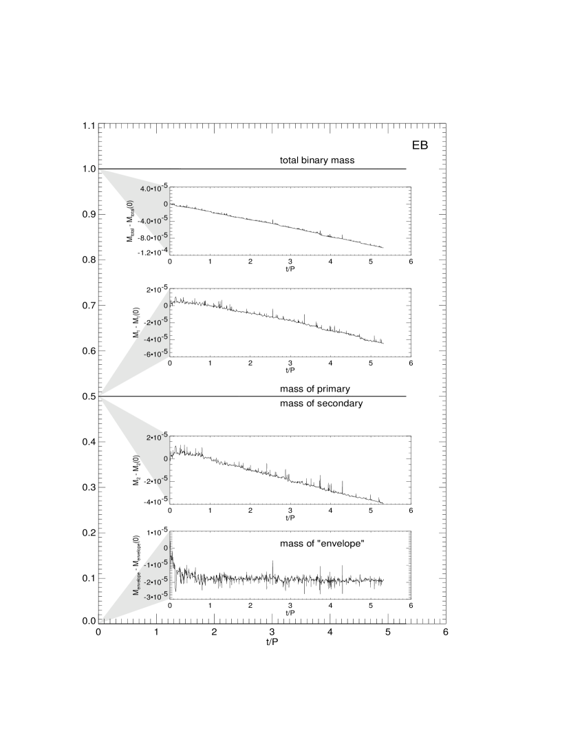
Figure 12: Masses, normalized to the total system mass, plotted as a function of time, in units of the orbital period, for the EB simulation. Top curve: Total binary mass ($M$). Middle two curves: Mass of the primary ($M_{1}$) and secondary ($M_{2}$) stars. Bottom curve (essentially at zero): Mass of the “envelope,” as defined in §6.2. Inset plots show the difference between the indicated mass component and its initial value in units of the initial total mass.

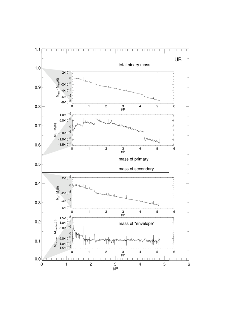
Figure 13: Masses, normalized to the total system mass, plotted as a function of time, in units of the orbital period, for the UB simulation. Top curve: Total binary mass ($M$). Middle two curves: Mass of the primary ($M_{1}$) and secondary ($M_{2}$) stars. Bottom curve (essentially at zero): Mass of the “envelope,” as defined in §6.2. Inset plots show the difference between the indicated mass component and its initial value in units of the initial total mass.

Although mass is conserved to very high precision, it is not absolutely constant throughout the evolutions. In the four insets of Figs. 12 and 13, we have magnified the vertical mass scale by roughly four orders of magnitude in order to show that there is a very tiny, but measurable, secular decrease in the total system mass and in the mass of both stellar components over the course of the simulations. In each inset, we plot the relevant mass minus its value in the initial state (time $t=0$), normalized to the total system mass. These inset plots show that the system mass decreases by approximately one part in $10^{4}$ over five orbits — that is, about $0.002\%$ per orbit — with the mass loss from each star accounting for roughly half this total. In rows $2-4$ of Table 6 we have recorded for both evolutions more precise values of the fractional mass that is lost, on average, each orbit from the primary ($M_{1}$), the secondary ($M_{2}$), and the system as a whole ($M$). We have determined that this mass is very slowly lost as a result of the development of a small, but nonzero flow of low-density material off of the stars, through the envelope and, ultimately, off of the grid. (After an initial drop, the envelope mass remains approximately constant, suggesting that this outward flow has settled into a nearly steady state.) As is discussed more fully in §7, below, this small but detectable rate of mass loss from detached equilibrium binaries imposes a straightforward limit on the mass-transfer rates that we will be able to reliably model in future simulations that involve dynamical mass transfer.

6.3 Minimal Center-of-Mass Motion

During both simulations we also tracked as a function of time the position of the center of mass of each binary component and the position of the center of mass of the system as a whole. The equatorial-plane trajectories of these three centers of mass for the EB and UB evolutions are shown, respectively, in Figs. 14 and 15, as viewed from our computational reference frame — that is, from a frame rotating with the orbital angular velocity of the system, as determined for the initial state by the SCF code. In the uppermost plot of each figure, which has been drawn at a scale ($-1<x<+1$; $-1<y<+1$) to include the entire mass of the system, the three separate center of mass trajectories appear to be small dots with little or no discernible structure. (When plotted in the inertial reference frame on this scale the trajectories of the two stars are indistinguishable from circles.) This illustrates that, even after five orbits, the centers of mass of the two stars and of the system as a whole essentially have not moved from their initial positions. This provides additional strong confirmation that our SCF code produces excellent initial states and that the hydrodynamical equations are being integrated forward in time in a physically realistic manner.

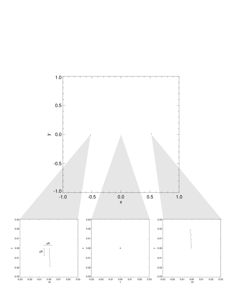
Figure 14: From the EB simulation, equatorial-plane trajectories are plotted for the center of mass of the system and the centers of mass of both stellar components through just over $5$ orbits in the corotating frame of reference. Insets (from left to right) show magnified views of the trajectories for the secondary star, the system as a whole, and the primary star. We have subtracted off the initial coordinates for the inset plots and have, for reference, indicated the size of one grid cell.

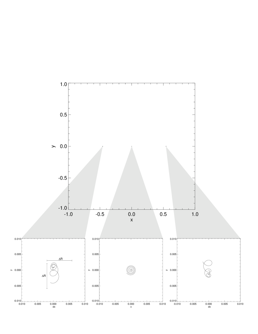
Figure 15: From the UB simulation, equatorial-plane trajectories are plotted for the center of mass of the system and the centers of mass of both stellar components through just over $5$ orbits in the corotating frame of reference. Insets (from left to right) show magnified views of the trajectories for the secondary star, the system as a whole, and the primary star. We have subtracted off the initial coordinates for the inset plots and have, for reference, indicated the size of one grid cell.

In the bottom three plots of Figs. 14 and 15, we have magnified a small region around each of the center of mass trajectories — expanding the linear scale of the uppermost plot in each figure by a approximately a factor of $15$ and $45$, respectively. These magnified views reveal that, although it is very small, there is measurable motion of the centers of mass in both evolutions. In the bottom, lefthand plot we also have shown the size of our radial grid spacing, $\Delta R=7.87\times 10^{-3}$. This indicates the characteristic size of our discretization and emphasizes how small the motion of each center of mass is. In the UB evolution, for example, the motion of all three centers has been confined within a single grid cell through five full orbits. Furthermore, the smooth spiral trajectory of the UB system center of mass (bottom, middle plot in Fig. 15) has an understandable, physical origin. As viewed in the inertial frame, this particular trajectory appears as a straight line whose direction and magnitude is consistent with the overall system velocity prescribed as initial conditions from eq. (60). In the EB evolution, due to the symmetry of the initial model, the drift of the system center of mass is extremely small, remaining unnoticable even on the magnified plot. In the magnified plots, the trajectory of the center of mass of each individual star shows both a gradual drift in the $y$-direction, and a small oscillatory motion in the $x$-direction. The vertical drift is mostly an indication that the binary’s actual orbital frequency is slightly different from the value (given by the SCF code) that we used for the rotation frequency of the computational grid. The oscillations in $x$ represent epicyclic motion and indicate that the binary orbit is not precisely circular. Since both the drift and the epicyclic motion can be understood in physical terms, their small amplitudes tell us more about the quality of the initial model than about the limiting accuracy of our finite-difference scheme.

Unlike in the single star case presented in §5.3, there is no evidence of a systematic outwards force on either star in the UB or EB systems, despite the fact that the systems have evolved for the equivalent of approximately 90 dynamical times. It appears as though the introduction of a rotating frame of reference and the associated centrifugal potential and Coriolis force has provided a feedback mechanism that acts to limit the systematic imbalance discussed previously.

6.4 Binary Separation

Figure 16: The orbital separation, normalized to its initial value, as a function of orbital time for the EB system.

Figure 17: The orbital separation, normalized to its initial value, as a function of orbital time for the UB system.

A plot of the binary separation $a$ as a function of time, as shown in Figs. 16 and 17 for the EB and UB evolutions, respectively, provides another way to assess the global behavior of these systems. Here, the separation $a$ is defined as the distance between the centers of mass of the two stars. Notice that, on a linear scale that extends from $0$ to $1$ (in units normalized to the each system’s initial separation), the plot of $a(t)$ is indistinguishable from a perfectly horizontal line. This illustrates that, to a very high degree of accuracy, these benchmark simulations of detached binary systems produce stable, circular orbits.

Again, though, if we examine these plots in finer detail, we see that both evolutions exhibit a very small but quantifiable departure from perfect circular orbital motion. For example, in the insets to Figs. 16 and 17, we have reploted $a(t)$ with the vertical scale magnified by roughly a factor of $400$. These insets show that in both evolutions there is a very slow, secular decrease in the orbital separation and, in addition, $a(t)$ displays low-amplitude oscillations having a period approximately equal to one orbital period. The oscillations in $a$ arise from the same epicyclic motion that was seen in the plots (Figs. 14 and 15) of the center of mass motion of the individual stars, but the amplitude of this motion is easier to measure here. In units of the initial orbital separation, the EB system has an epicyclic amplitude $(\Delta a/a)_{\rm epicyclic}\approx 5\times 10^{-4}$; the UB system exhibits an epicyclic amplitude about half this size. The slow, secular decay of the orbits occurs at a rate $({\Delta a}/{a})_{\rm secular}\approx 2.9\times 10^{-4}$ per orbit in the EB system, and at a rate ${\Delta a}/{a}\approx 1.9\times 10^{-4}$ per orbit in the UB system. These orbital decay rates and epicyclic amplitudes have been recorded in the fifth and sixth rows of Table 6.

6.5 Angular Momentum Conservation

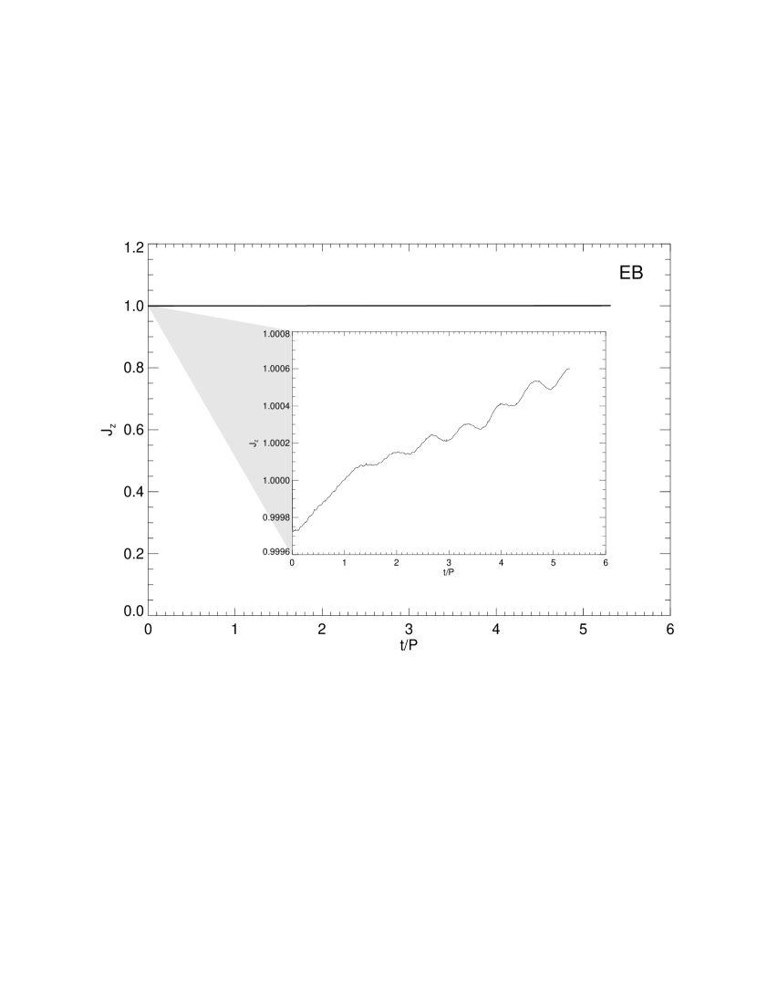
Figure 18: The z component of total angular momentum, normalized to its initial value, as a function of time for the EB system.

Figure 19: The z component of total angular momentum, normalized to its initial value, as a function of time for the UB system.

Finally, in Figs. 18 and 19 we show the behavior as a function of time of the $z$-component of each system’s total angular momentum. As was true with our plots of the orbital separation, on a linear scale that extends from $0$ to $1$ (in units normalized to the each system’s initial total angular momentum), the plot of $J_{z}(t)$ is indistinguishable from a perfectly horizontal line. This illustrates that these benchmark simulations globally conserve angular momentum to a very high degree of accuracy. When we magnify the vertical scale by approximately a factor of $1000$, as has been done to produce the insets to Figs. 18 and 19, we see that angular momentum is not, in fact, perfectly conserved. Evidently both systems gain angular momentum at a very slow rate; in the EB simulation, ${\Delta J_{z}}/{J_{z}}\approx 1.1\times 10^{-4}$ per orbit, and in the UB simulation ${\Delta J_{z}}/{J_{z}}\approx 1.5\times 10^{-4}$ per orbit. These rates have been recorded in the seventh row of Table 6 and will be referred to again in §7, below, when we summarize the limiting accuracy with which we expect to be able to model physical mass-transfer events using our simulation tools.

6.6 Overview

We should emphasize that the hydrodynamics code as described in §4 and utilized in these benchmark simulations has evolved through many stages from the version of the code that was used several years ago by New & Tohline (1997) to investigate the equal-mass, binary merger problem. A number of improvements were made in the code in order to bring it to its present level of performance. Figure 20 is presented here in an effort to illustrate how certain key modifications in the code affected its performance. Each row of frames in this figure shows results from an evolution of the same unequal-mass (UB) binary system that was used in our benchmark simulation, but as produced by four separate versions of the code. The curves drawn in the four frames on the left-hand side of Fig. 20 show the same type of information as has been presented in Fig. 10 for the benchmark UB evolution: Four separate volumes for the secondary star (solid curves) and its Roche volume (dashed curve) are plotted as a function of time, in units of the orbital period. The four frames on the right-hand side of Fig. 20 show the same type of information as has been presented in the top-most frame of Fig. 15: Center-of-mass trajectories of the two stars and of the system as a whole, as viewed from the rotating frame of reference. (The bottom-most frames are taken from the benchmark UB simulation and therefore are drawn directly from Figs. 10 and 15.)

Figure 20: Each of the four pairs of plots shown here has been derived from the UB simulation as modeled with one of four separate versions of our hydrodynamic code. In each pair, the plot on the left is directly analogous to Fig. 10, showing as a function of time the Roche volume (dashed curve) and four interior volumes (solid curves) for the secondary star; the plot on the right is directly analogous to the unmagnified plot in Fig. 15, showing the trajectories of the center of mass of the secondary (left), system as a whole (center), and primary (right). The pairs of plots are shown chronologically from the top to the bottom, with significant improvements in the code being made between each recorded UB simulation. See §6.6 for a description of these various code improvements.

The results shown in the top-most frames of Fig. 20 come from an early version of the code in which we replaced the gradient of the pressure with the gradient of the enthalpy. This ensured that the initial structure of each star, as determined by the SCF code, was in good force balance after being introduced into the hydrocode. However, as the two figures from this evolution illustrate, we still observed a slow expansion of the secondary star; the orbit itself developed a significant epicyclic amplitude; and after about three orbits, the Roche lobe was encroaching on the surface of the secondary. The second row of frames comes from a simulation in which the number of azimuthal zones was doubled — from 128 to 256 zones over the full $2\pi$ radians. This modification improved somewhat the mean motion of the centers of mass (although it did not significantly reduce the amplitude of the epicyclic motion). Most significantly, however, doubling the angular grid size improved the resolution and, hence, the determination of force balance in each star. As a result, expansion of the secondary star was noticeably reduced. The third row of frames shows that motion of the centers of mass was drastically reduced when we modified our algorithm to make the integration scheme more properly time-centered. This change did not noticeably reduce the rate of expansion of the secondary, but it did significantly reduce the amplitude of oscillations in the Roche lobe volume. Finally, by introducing artificial viscosity into the equations of motion in order to mediate the weak shocks at the surface of the stars (which also involved a re-centering of all momentum densities to the cell locations specified in Table 3), the entire structure of both stars became much more robust. In particular, as the left-hand frame of the last row shows (see also Fig. 10), this code modification completely eliminated the short timescale wiggles in the volumes of the secondary; overall expansion of the secondary also was reduced to an imperceptible level. Simultaneously, for the first time, we ascribed a small nonzero velocity to the initial state as given by eq. (60). This change further reduced the motion of the centers of mass — to the level illustrated by Fig. 15.

It is reasonable to ask whether the three principal spurious effects that remain in our benchmark simulations — the slow decay of the orbits, the slow gain of angular momentum, and the slow loss of mass from the stars — are at least mutually consistent on physical grounds. For centrally condensed binaries, a point mass approximation (the Roche approximation) is usually sufficient to discuss the orbital evolution. This approximation predicts a simple relationship between the changes of mass, angular momentum and binary separation, namely

$$\frac{\Delta J_{\rm com}}{J_{\rm com}}=\frac{1}{2}\frac{\Delta a}{a}+\frac{\Delta M_{1}}{M_{1}}+\frac{\Delta M_{2}}{M_{2}}-\frac{1}{2}\frac{\Delta M}{M}\,,$$ (61)

where $J_{\rm com}=M_{1}M_{2}\sqrt{Ga/M}$ is the total center–of–mass angular momentum in the point mass approximation. Numerical values for each of the terms in this expression can be obtained from the data shown in Table 6. In particular, we see that in both benchmark simulations the three mass terms approximately cancel each other out. But while the magnitude of $(\Delta a/a)_{\rm secular}$ is roughly the same as the magnitude of $\Delta J_{z}/J_{z}$, their signs are different. That is, the angular momentum of the system is slowly increasing while the binary separation is slowly decreasing. This is clearly inconsistent with the expectations of the simple Roche model. A more accurate expression for the total angular momentum of the binary would be

$$J_{\rm bin}=J_{\rm com}+I_{1}\Omega_{1}+I_{2}\Omega_{2}\,,$$ (62)

where $I_{i}$ and $\Omega_{i}$ are the moments of inertia and inertial frame angular velocities of the binary components, assuming they all rotate around the same $z$-axis. Even if one takes into account the contributions of spin angular momenta, the changes observed remain inconsistent and must therefore be attributed to spurious numerical effects at a level of $10^{-4}$ per orbit arising from the inevitable error terms present in our finite-difference representation of the fluid equations. What we have attempted to do here is quantitatively document the magnitude of these numerical effects in the highest practical resolution possible at the present day for simulations of detached binaries where the character of the ideal solution is well understood beforehand. Furthermore, we can not accurately predict the evolution of mass transferring binaries where the mass transfer rate, ${\Delta M}/{M}$ per orbit is $\lesssim{\rm few}\times 10^{-5}$ using simulations at the resolution presented here. There are however a wide variety of systems (the initial mass transfer event in an Algol progenitor, or the onset of common envelope evolution in the progenitors of many types of binaries, or the formation of Type Ia supernovae for example) that are expected to exceed our threshold resolution limit for mass transfer. At a sufficiently high mass-transfer rate, the mass transfer itself will drive the evolution of the orbital parameters and Roche geometry at a rate higher than the numerical limits demonstrated here.

7 Conclusions

In this paper we have presented a practical SCF algorithm for constructing self-consistent polytropic binaries with unequal masses that satisfy the condition of hydrostatic equilibrium to a high degree of accuracy. This three-dimensional SCF algorithm is based largely on the technique first described by Hachisu (1986), but to our knowledge this is the first time the technique has been used to generate unequal mass binary systems as input for a hydrodynamical simulation. Our two benchmark simulations (described in §6) clearly indicate that this SCF algorithm can provide superb initial states for investigations into the dynamical stability of close binary systems. We emphasize that, in addition to generating models of close binary systems that are detached — like the EB and UB systems constructed for our two benchmark simulations — as shown above in Figs. 2 and 3 this technique also can be used to generate close binary systems that are semi-detached or, in the limit of identical components, in contact.

We have also detailed our gravitational hydrodynamics code and presented results from key tests of the stability and accuracy of the hydrodynamics algorithm, the solution of Poisson’s equation, and the coupled solution required to evolve an isolated, spherical polytrope that is placed off-axis in a cylindrical grid. From these test cases it is apparent that a number of subtle numerical issues arise when a highly nonaxisymmetric body is evolved via an explicit integration of finite-difference equations on a cylindrical computational grid. It also appears however, that these effects can be made manageably small by increasing the resolution used to treat the system of interest.

We have evolved two detached binary systems (one with a mass ratio $q=1$, the other with a mass ratio $q=0.8436$) through more than five orbits in order to benchmark in detail the capabilities of our simulation tools. Even though the individual stellar components generated by our SCF code are significantly rotationally flattened (due to the synchronous rotation of the initial states) and tidally distorted (by their close binary companion), these benchmark simulations show that the stars are in almost perfect hydrostatic equilibrium. Throughout each binary evolution, our hydrodynamics code conserves mass and angular momentum to a very high degree of precision; as viewed from a frame of reference that is rotating with the initial orbital frequency of the binary, the centers of mass of the two stellar components and of the system as a whole remain virtually stationary; and a plot of the binary separation as a function of time shows that the stellar orbits are almost indistinguishable from circles. This gives us considerable confidence that these numerical tools can be used to examine the stability of close binary systems against both tidal and mass-transfer instabilities, and to begin to accurately model mass transfer in semi-detached systems.

As has been summarized in Table 6, from our benchmark evolutions we have been able to determine in quantitative terms the level of accuracy with which our hydrodynamical code conserves mass, conserves angular momentum, and is able to represent and maintain a circular binary orbit. Mass is conserved to roughly $0.002\%$ per orbit; angular momentum is conserved to a level of $0.01$ - $0.02\%$ per orbit; the binary separation remains constant to a few parts in $10^{4}$ per orbit; and each orbit exhibits an epicyclic amplitude (measured relative to the orbital separation) of $.02$-$.05\%$.

We are unaware of any other group that is attempting to study the onset of mass-transfer instabilities in unequal-mass binaries with a gravitational hydrodynamics code, like ours, that fully resolves both stellar components. Hence, there are no published numbers against which to compare ours for the UB evolution. However, we can fairly compare the results of our EB evolution against the recent study published by SWC of equal-mass close binary systems. Their Fig. 10 illustrates that, after following one stable binary system through approximately $6$ orbits (we assume, based on the SWC discussion, that $P=1.7-2\ {\rm ms}$), they have been able to conserve angular momentum to a level of about $0.2\%$ per orbit. And their Fig. 14 shows four stable orbits with epicyclic amplitudes (measured relative to the binary separation) $\sim 0.3-1\%$. We conclude that, at least in these two respects, our simulations improve on the SWC models by roughly one order of magnitude. SWC do not comment on their level of mass conservation; and, because of the visible epicyclic motions in their Fig. 14, it is difficult to ascertain to what degree the binary separation either decreases or increases with time over the course of their evolutions. In both of our evolutions, however, the center-of-mass motion of our stars appears to be significantly less than the center-of-mass motion depicted for SWC’s preferred integration scheme in the top-left panel of their Fig. 7.

The small, but measurable changes in mass, angular momentum, and binary separation documented here in Table 6 set limits on the types of mass-transfer events that we will be able to model with confidence using our present simulation tools. For example, if we were to try to model an instability that leads to a flow through the binary’s L1 Lagrange point with a mass-transfer rate lower than one part in $10^{6}$ per orbit, the physical exchange of material between the binary components would be swamped by the unphysical process that is causing our stars to lose mass to the “envelope” at a rate of one to two parts in $10^{5}$ per orbit. If the depth of contact between the Roche lobe and the surface of the donor star is not sufficient, epicyclic motion in the orbit will tend to shut off the mass-transfer during part of each orbit. Also, a drift in the center of mass of the system can impose a limit on the length of time that the binary can be evolved before the motion of the binary through the grid becomes problematic. We will have to contend with all of these issues as we move to the next level of our investigation and introduce a semi-detached system from our SCF code into our hydrodynamical code. We expect nevertheless to find a wide range of interesting binary systems whose dynamical evolution can be simulated in a fully self-consistent fashion through a reasonably large number of orbits using the tools that have been described in this paper.

As we have documented in Table 6, the calculation of one orbit takes about 33 wall-clock hours when utilizing 64 processors of the Cray T3E 600, and using 16 processors of the newer IBM SP-3, the calculation of one orbit takes about 51 hours. The computational workload of a mass-transfer simulation is therefore within the reach of current, state of the art, parallel computers given the linear scaling of our gravitational hydrodynamics code with the number of processors even at a resolution greater than presented here. We note that the amount of work performed can be reduced significantly if need be by, for example, freezing the gravitational potential until the mass distribution has changed significantly as done by Stone & Norman (1992). The solution of Poisson’s equation represents about a quarter of the total execution time.

We have been able to estimate the mass transfer rate required to bring the simulation above the level of the noise observed in our benchmark simulations. We find that this value is $\sim\mathrm{few}\times 10^{-5}$ of the donor’s initial mass over an orbital period. As discussed in §2, the mass transfer rate should scale as a high power of the degree of over-contact (as the cube for an $n=3/2$ polytrope); furthermore, for a case where $q>1$, that is, the donor is initially the more massive star, the degree of over-contact will naturally increase with time as the star expands and its Roche lobe shrinks. Provided that such a binary system can begin mass-transfer, the amplitude of the mass transfer rate should inevitably reach values higher than indicated above. Since motion of the center of mass of the binary system has been confined to a region well within a single computational grid cell even after $5$ orbits, we are confident that future evolutions can be followed with confidence through at least $20-30$ orbits, given sufficient computing resources. As discussed in the introduction of this paper, we understand that the mass transfer rates considered here are much larger than those found in what are considered typical examples of interacting binaries. The methods presented here are not applicable to the stable mass transfer observed in cataclysmic variables or other long lived systems, but should serve very well to investigate stages of evolution of their progenitors and transient events such as the onset of dynamical mass transfer and its stability.

References

- Batten (1989) Batten, A. H. 1989, Proc. IAU Coll. Nr. 107, Algols (Dordrecht:Kluwer Academic Publishers)
- Bhattacharya (1995) Bhattacharya, D. 1995, in X-Ray Binaries, ed. W. H. G. Lewin, J. van Paradijs, & E. P. J. van den Heuvel (Cambridge: Cambridge University Press), 233
- Bisikalo et al (2000) Bisikalo, D. V., Harmanec, P., Boyarchuk, A. A., Kuznetov, O. A., & Hadrava, P. 2000, A&A, 353, 1009
- Black & Bodenheimer (1975) Black, D. C., & Bodenheimer, P. 1975, ApJ, 199, 619
- Blondin, Richards & Malinowski (1995) Blondin, J. M., Richards, M. T., & Malinowski, M. L. 1995, ApJ, 445, 939
- Boroson et al (2001) Boroson, B., Kallman, T., Blondin, J. M., & Owen, M. P. 2001, ApJ, 550, 919
- Bowers & Wilson (1991) Bowers, R. L., & Wilson, J. R. 1991, Numerical Modeling in Applied Physics and Astrophysics (Boston:Jones and Bartlett)
- Cazes & Tohline (2000) Cazes, J. E., & Tohline, J. E. 2000, ApJ, 532, 1051
- Chandrasekhar (1939) Chandrasekhar, S. 1939, An Introduction to the Study of Stellar Structure (Chicago: University of Chicago Press)
- Cohl, Sun & Tohline (1997) Cohl, H. S., Sun, X.-H., & Tohline, J. E. 1997, in Proceedings of the 8th SIAM conference on Parallel Processing for Scientific Computing, ed. M. Heath, V. Torczon, G. Asffalk, P. E. Bjørstad, A. H. Karp, C. H. Koebel, V. Kumar, R. F. Lucas, L. T. Watson, & D. E. Womble (Philadelphia: SIAM)
- Cohl & Tohline (1999) Cohl, H. S., & Tohline, J. E. 1999, ApJ, 527, 86
- Frank, King & Raine (2001) Frank, J., King, A. R., & Raine D. J. 2001, Accretion Power in Astrophysics, (3rd ed:Cambridge: Cambridge University Press), in press
- Hachisu (1986) Hachisu, I. 1986, ApJS, 62, 461
- Hachisu, Eriguchi & Nomoto (1986) Hachisu, I., Eriguchi, Y., & Nomoto, K. 1986, ApJ, 311, 214
- Hawley, Wlison & Smarr (1984) Hawley, J. F., Wilson, J. R., & Smarr, L. L. 1984, ApJS, 55, 211
- Iben & Livio (1993) Iben, I., Jr., & Livio, M. 1993, PASP, 105, 1373
- Iben & Tutukov (1984) Iben, I., Jr., & Tutukov, A. V. 1984, ApJS, 54, 335
- Iben (1990) Iben, I., Jr. 1990, ApJ, 353, 215
- Janka et al (1999) Janka, H.-T., Eberl, T. Ruffert, M. & Fryer, C. L. 1999 ApJ, 527, L39
- King et al (1997) King, A. R. Frank, J. Kolb, U. & Ritter, H. 1997, ApJ, 482, 919
- Lai, Rasio & Shapiro (1994) Lai, D. Rasio, F. A. & Shapiro, S. L. 1994, ApJ, 423, 344
- Lewin, van Paradijs & van den Heuvel (1995) Lewin, W. H. G. van Paradijs, J. & van den Heuvel, E. P. J. 1995 X-Ray Binaries, (Cambridge: Cambridge University Press)
- Lindblom, Tohline & Vallisneri (2001) Lindblom, L. Tohline, J. E. & Vallisneri, M. 2001, Phys. Rev. Lett., 86, 1152L
- Lufkin & Hawley (1993) Lufkin, E. A. & Hawley, J. F. 1993, ApJS, 88, 569
- Marietta, Burrows & Fryxell (2000) Marietta, E. Burrows, A. & Fryxell, B. 2000, ApJS, 128, 615
- Mészáros (2001) Mészáros, P. 2001, Science, 291, 79
- Nelson & Eggleton (2001) Nelson, C. A. & Eggleton, P. P. 2001, ApJ, 552, 664
- New & Tohline (1997) New, K. C. B. & Tohline, J. E. 1997, ApJ, 490, 311
- New, Centrella & Tohline (2000) New, K. C. B. Centrella, J. M. & Tohline, J. E. 2000, Phys. Rev. D, 620, 13
- Norman & Winkler (1983) Norman, M. L., & Winkler, K.-H. 1983, in Astrophysical Radiation Hydrodynamics, ed. K.-H. Winkler and M. L. Norman (Dordrecht:Reidel), 449
- Paczyński (1971) Paczyński, B. 1971, ARA&A, 9, 183
- Paczyński (1986) Paczyński, B. 1986, ApJ308, L43
- Paczyński and Sienkiewicz (1972) Paczyński, B. & Sienkiewicz, R. 1972, Acta Astronomica, 22, 74
- Peaceman & Rachford (1955) Peaceman, D. & Rachford, H. 1955, J. Soc. Indust. Appl. Math., 3, 28
- Ruffert et al (1997) Ruffert, M., Janka, H.-T., Takahashi, K., & Schaefer, G. 1997, A&A, 319, 122
- Sandquist et al (1998) Sandquist, E. L., Taam, R. E., Xingming, C., Bodenheimer, P., & Burkert, A. 1998, ApJ, 500, 909
- Schwarztrauber & Sweet (1975) Schwarztrauber, P., & Sweet R. 1975, in Efficient FORTRAN Subroutines for the Solution of Elliptic Partial Differential Equations, NCAR Technical Note - TN/IA-109
- Schwarztrauber et al (2001) Schwarztrauber, P., Sweet, R., & Adams, J. http://www.scd.ucar.edu/css/software/fishpack
- Stone & Norman (1992) Stone, J. M., & Norman, M. L. 1992, ApJS, 80, 753
- Sod (1978) Sod, G. 1978, J. Comput. Phys., 27, 1
- Swesty et al (2000) Swesty, F. D., Wang, E. Y. M., & Calder, A. C. 2000, ApJ, 541 937 (SWC)
- Trimble (1983) Trimble, V. 1983, Nature, 303, 137
- van Leer (1979) van Leer, B. 1979, J. Comput. Phys., 32, 101
- Verbunt & van den Heuvel (1995) Verbunt, F., & van den Heuvel, E. P. J. 1995, in X-ray Binaries, ed. W. H. G. Lewin, J. van Paradijs, & E. P. J. van den Heuvel (Cambridge: Cambridge University Press), 457
- Vesper, Honeycutt & Hunt (2001) Vesper, D., Honeycutt, K., & Hunt, T. 2001, AJ, 121, 2723
- Warner (1995) Warner, B. 1995, Cataclysmic Variable Stars, (Cambrdige: Cambridge University Press)