Twenty Years of Timing SS433

Abstract

We present observations of the optical “moving lines” in spectra of the Galactic relativistic jet source SS433 spread over a twenty year baseline from 1979 to 1999. The red/blue-shifts of the lines reveal the apparent precession of the jet axis in SS433, and we present a new determination of the precession parameters based on these data. We investigate the amplitude and nature of time- and phase-dependent deviations from the kinematic model for the jet precession, including an upper limit on any precessional period derivative of $\dot{P}<5\times 10^{-5}$. We also dicuss the implications of these results for the origins of the relativistic jets in SS433.

1 Introduction

SS433 is the first known example of a Galactic relativistic jet source, and thus the forerunner of modern microquasar astrophysics. The optical spectrum of this object shows a number of strong, broad emission lines of the Balmer and HeI series, as well as several lines at unusual wavelengths. These latter have been identified as red/blue-shifted Balmer and HeI emission from collimated jets with intrinsic velocities of $v\simeq 0.26c$ (Abell & Margon, 1979). Furthermore, the Doppler shifts of these features change with time in a cosinusoidal manner, leading to the label of “moving lines”. This behavior is now widely accepted to be a symptom of precession of the jet axis in SS433 on a timescale of $\sim 164$ days (Margon, 1984).

Early studies of the precession in SS433 indicated possible instabilities or drifts in the precessional clock (Anderson et al., 1983), which could give considerable insight into the accretion processes which must provide the precessional torque. However, Margon & Anderson (1989) reviewed ten years of SS433 timing data and concluded that while significant deviations from cosinusoidal behavior exist in SS433, the evidence for systematic long-term drifts (e.g. precessional period derivative, $\dot{P}$) remained inconclusive.

In this paper, we take the data set considered by Margon & Anderson (1989) and add to it more than 50 Doppler shift measurements spread over 10 years, including 9 Doppler shifts measured in 1999. Combined, these observations span more than 20 years, and thus provide an excellent data set for constraining long-term drifts in SS433’s precessional clock. We discuss the observations in Section 2. In Section 3, we present analyses of the entire data set in the context of the “kinematic model” for SS433’s precessing jets. In Section 4, we discuss the results of these analyses, and in Section 5 we present our conclusions.

2 Observations

The primary observations used here are optical spectroscopic observations of SS433, from a wide range of telescopes and instruments (see Margon & Anderson (1989) and references therein for details). The net result of these observations, spread over the period from June 1978 to July 1992, is the measurement of 433 Doppler shifts for the “receding jet” ($z_{1}$) and 482 Doppler shifts for the “approaching jet” ($z_{2}$) for the optical moving lines in SS433.

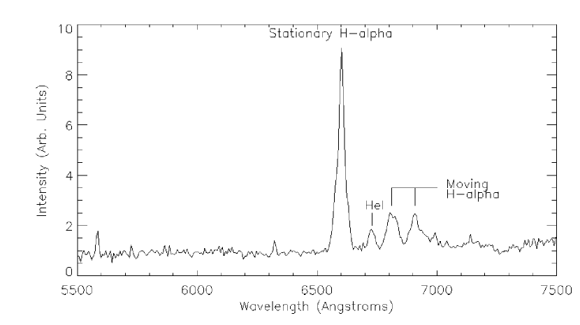
Figure 1: Typical spectrum of SS433 taken from the Hartung-Boothroyd Observatory 24-inch telescope. Note the clear appearance of the moving Balmer lines from the jets.

We obtained further spectra of SS433 in July, 1999 using the Hartung-Boothroyd Observatory (HBO) 24-inch telescope and optical CCD spectrograph. We used a 600 lines/mm grating and $6\arcsec$ slit providing a resolution of $R\sim 800$ ($6\ {\rm\AA/pix}$). We present a typical spectrum in Figure 1.

We determined the Doppler shift of each HBO spectrum using only the moving $H\alpha$ lines, and we did so by fitting a Gaussian profile to the red and blue components separately. Note that the profiles of the moving lines are broad, time-variable, and often asymmetric. This is due to the time overlap of multiple discrete emission components, commonly referred to as “bullets” (Vermeulen et al., 1993), with typical lifetimes of $\sim 3$ days. These systematic deviations introduce a relatively large uncertainty in the Doppler shift determination. Based upon examination of many spectra, we find that the typical full-width at half-maximum (FWHM) is $\Delta z\sim 0.003$, and we adopt this as our uncertainty in the Doppler shift determination $\sigma_{z}$.

3 Analysis

3.1 The Kinematic Model

Throughout our analysis of these data, we adopt the “kinematic model” for the moving lines, which assumes that the changing Doppler shifts arise from the precession of the jet axis in SS433. The simplest form of the kinematic model takes into account five components: the jet velocity $\beta={v\over{c}}$; the jet angle from the precessional axis $\theta$, the inclination angle of the system with respect to the observer’s line of sight $i$, the precession period $P$, and the epoch of zero precessional phase $t_{0}$. The period and zero-phase epoch combine to give the precessional phase $\phi={{t-t_{0}}\over{P}}$. The resulting Doppler shifts obey the equation

$$z_{1,2}=1-\gamma[1\pm\ \beta\ \sin\theta\ \sin i\ \cos\phi\ \pm\ \beta\ \cos\theta\ \cos i]$$

where $\gamma=(1-\beta^{2})^{-1/2}$. SS433 exhibits “nodding” of the jets on a $\sim 6.5$-day period (Katz et al., 1982) due to the $\sim 13$-day binary motion of SS433 (Crampton et al., 1980), which are not accounted for in this model. However, the effects of this nodding are essentially negligible for long timescale studies of the jets such as ours. We further mitigate the impact of nodding by applying a 7-day boxcar smoothing filter to the individual Doppler shifts determined above. We then used chi-squared minimization to find the best-fit parameters for the kinematic model (Table 1). The resulting model fit is plotted versus time along with the data and residuals in Figures 2-3 for $z_{1}$ and $z_{2}$. We plot the same model fit, data, and residuals versus precessional phase in Figure 4.

The resulting fit has a chi-squared residual per degree of freedom of $\chi^{2}_{\nu}=8.9$, indicating the presence of statistically significant residuals. However, we can still use this fit to estimate uncertainties in the kinematic model parameters as follows. First, we scale all of the $\sigma_{z}$ values by $\sqrt{8.9}$, so that the residuals have $\chi^{2}_{\nu-fix}=1.0$, essentially by fiat. We then take the uncertainties to be the range of a model parameter which introduces a total change of $\Delta\chi^{2}_{fix}=1.0$. We also report these values in Table 1. This rescaling approach for deriving the model parameter uncertainties is statistically valid in a strict sense only if the residuals are consistent with Gaussian noise and are not correlated with any model parameters in a systamtic way. If so, then the residuals would simply indicate that we have ignored one or more sources of noise in the system when estimating the uncertainties in the individual Doppler shifts. As we show below, this is largely true, though we see some evidence of small (but statistically-significant) systematic deviations from the kinematic model. Thus, the uncertainties in the model parameters in Table 1 are likely to be good, but not perfect, statistical estimates. For the remainder of the paper, we adopt the best-fit model parameters presented in Table 1.

3.2 Doppler Shift Residuals

One obvious feature of Figures 2-4 is that the residuals to the model fit greatly exceed the uncertainties in the Doppler shift determinations (as also shown by the large value of $\chi^{2}_{\nu}$ above). We also notice no obvious trend in the residuals versus time as would be expected for systematic timing effects, such as a constant precessional period time derivative $\dot{P}$. Such large, apparently random residuals have been noticed in previous timing studies of SS433 (Anderson et al. (1983); Margon & Anderson (1989)).

3.2.1 Correlations in Residuals

Previous studies have also noticed that the velocity residuals in SS433 show a pattern of correlation between $z_{1}$ and $z_{2}$ (Margon & Anderson, 1989). Specifically, when we plot the residuals of $z_{1}(obs)-z_{1}(mod)$ versus $z_{2}(obs)-z_{2}(mod)$, we find that most of the points lie in the second and fourth quadrants (Figure 5). In other words, when the absolute value of $z_{1}$ is greater than expected, the absolute vlaue of $z_{2}$ is also greater than expected, and vice versa. The number of data points with $z_{1}$ and $z_{2}$ residuals in quadrants 2 and 4 is $271\pm 16$, while in quadrants 1 and 3 the number is $110\pm 10$ – a $>8\sigma$ difference.

The linear correlation coefficient between the residuals is $r=-0.69\pm 0.02$. We estimate the uncertainty from a Monte Carlo simulation as follows. We take the 381 pairs of $z_{1}$ and $z_{2}$ residuals and add to each a random number drawn from a Gaussian distribution with mean of zero and a standard deviation of 0.003 – the typical uncertainty in the Doppler shift measurements. We then calculate the correlation coefficient of the resulting simulated distribution. We repeat this procedure 1000 times and then take the standard deviation in the correlation coefficient as the uncertainty above, $\sigma_{r}=\pm 0.02$.

This correlation pattern could have several physical sources. The effect considered most commonly in previous studies (e.g. Margon & Anderson (1989)) is that of phase noise in the precessional motion, with strict symmetry between $z_{1}$ and $z_{2}$. As the jet precessional phase either lags or leads the model ephemeris, the projected velocity amplitudes of the jets on the observers line of sight will either exceed or fall short of the model prediction. Another possible physical explanation is modulation of the velocity amplitude – “$\beta$-noise” – in a system which otherwise follows the 5-parameter kinematic model ideally (e.g. Milgrom et al. (1982)).

3.2.2 Phase-Dependence of Residuals

Another factor which could impact the $z_{1}/z_{2}$ residual correlation are phase-dependent residuals to the kinematic model. Margon & Anderson (1989) found no evidence for such phase-dependence in their data. In analyzing this data set, we divided the data into 10 evenly-spaced phase intervals and calculated the average and standard deviation of the residual Doppler shifts in each bin (Table 2). None of the average residuals from the kinematic model is as large as the rms deviation for residuals in that phase bin, indicating that phase-dependent deviations from the kinematic model do not dominate the residuals. Furthermore, if we compare the average residuals of the individual phase bins to the rms scatter of all the phase bins, none of them are more than $2\sigma$ outliers. Thus, the amplitude of any average deviation from the model velocity does not seem to be phase-dependent.

However, when we calculate the uncertainty in the average residual for each phase bin, equal to the standard deviation in the residuals divided by the square-root of the number of points, we find that the deviations are in fact statistically significant (Table 2). That is, while the scatter around the kinematic model in any given phase bin is not dominated by systematic deviations from the model, such deviations are present in the data set. The nature of these systematic deviations are not clearly determined. Figures 2-3 show that the velocity residuals show some correlation on timescales of weeks or months. Thus, sparse sampling of the velocities combined with such correlations in the residuals could be one explanation for the apparent systematic deviations.

We used the average residuals from the kinematic model as correction factors for the quadrant analysis presented above and in Figure 5, taking the observations and subtracting both the kinematic model and the average deviation for all points within $\Delta\phi=\pm 0.05$ cycles of each data point. As a result, the number of $z_{1}$,$z_{2}$ residual pairs in quadrants 2 and 4 does decrease, but only to 261 (with 120 pairs in quadrants 1 and 3). Thus the correlation between $z_{1}$ and $z_{2}$ residuals remains highly statistically significant even after correction for the systematic deviations.

We also note that the relative phase-independence of the residuals raises questions regarding the nature of the residuals. As can be seen from the equation for Doppler shifts in the kinematic model, every parameter which could be time-variable ($\beta,P,i,\theta,$) either feeds directly into the phase $\phi$ or is multiplied by $\cos\phi$. Thus, noise in these terms or in $\phi$ itself should result in a cosinusoidal modulation in the RMS of the Doppler shift residuals with $\phi$.

3.2.3 The Phase Noise Model

As mentioned above, the most commonly-invoked physical model for the velocity residuals in SS433 is “phase jitter” in the jet precession. Since the precession phase affects both jets similarly, it naturally explains the correlation between the $z_{1}$ and $z_{2}$ residuals. If such jitter can occur over timescales of weeks or months, it can also explain the long-term residual correlations evident in Figures 2-3.

We analyzed this SS433 data set following the example of Margon & Anderson (1989), determining phase errors from the velocity residuals above. We simply defined the phase error to be the phase difference between the actual phase of the observation given its epoch and the kinematic model parameters in Table 2 and the closest model point with the same observed velocity. As can be seen in Figure 4, some observed velocity amplitudes exceed the maximum model velocity amplitude, and such points were dropped from this analysis. We then divided the data set into 10-day intervals and calculated the average and standard deviation of the phase errors from all phase measurements doing that interval (including both $z_{1}$ and $z_{2}$). For 10-day intervals with only 1 phase measurement we have no estimate of the standard deviation, and thus dropped such intervals from the analysis. We plot the resulting phase noise measurements in Figure 6. We repeated this same analysis using a 30-day interval for averaging, with the results shown in Figure 7.

We note that while there are occasional trends in the residuals on timescales of several hundred days, no obvious trend is apparent over the full time span in either panel of Figure 7. The 1999 data are marginally inconsistent with zero phase residual (at the $2.8\sigma$ level for one of the two data points in Figure 6b). However, it is clear that this phase residual is less than many prior apprently secular deviations from the kinematic model in Figures 6-7. If we assume that some period derivative is present in SS433 over the span of our observations, these secular deviations could mask its effects up to $\Delta\phi\sim 0.05$ cycles. Given the span of our observations, this corresponds to an upper limit on the period derivative of $\dot{P}<5\times 10^{-5}$.

3.2.4 The Velocity Amplitude Noise Model

As mentioned above, an alternate physical explanation for the velocity residuals in Figures 2-4 is noise in the intrinsic velocity of the jets. To investigate this possibility further, we calculated the intrinsic jet velocity necessary to match each observed Doppler shift, given $\theta,\ i,\ t_{0},\ {\rm and}\ p$ from the best-fit parameter set in Table 1. We plot the corresponding values for $\beta={v\over{c}}$ versus time in Figure 8 and versus precessional phase in Figure 9.

The average value of $\beta$ we find is 0.254 with a standard deviation of $0.024$. Given 507 independent measurements of $\beta$ in this way, we arrive at an average value of $\beta_{ave}=0.254\pm 0.0011$. While this value is only $\sim 4\%$ lower than the value given in Table 1, the difference is statistically significant at the $7.9\sigma$ level. This may indicate that “noise” in the Doppler shifts may in fact be impacting the parameter estimates for the kinematic model in a systematic way, as discussed in Section 3.1.

4 Discussion

4.1 Phase Noise

As noted above, the upper limit on precessional period derivative of $\dot{P}<5\times 10^{-5}$ shows that there is no large long-term drift in the precessional timing properties of SS433. The presence of jitter in the system implies some “torque noise” in the process driving the precession, according to the phase noise model. However, if this were the case, that noise must average out over timescales of $\sim 20$ years. We can also see from Figure 7 that there are fairly large phase deviations of $\Delta\phi\sim 0.1$ cycles over timescales as short as $\sim 10$ days. This implies that the torque noise $\Delta\tau$ has a maximum relative amplitude of at least

$${\Delta\tau_{max}\over{\tau}}\simeq{{(\Delta\phi/\Delta t)}\over{(\partial\phi/\partial t)}}$$

$$\simeq 1.6$$

Thus, the variation in torque can in fact exceed the time-averaged torque driving the precession. This may be a problem for certain physical models of the precession and timing noise in SS433.

Finally, we note that the phase noise model is incapable of producing the observed Doppler shifts which exceed the maximum amplitude predicted by the kinematic model. We have considered the possibility that the phase noise itself causes the $\chi$-squared fitting procedure used to determine the model parameters to systematically underestimate the true jet velocity, and thus “undershoot” the maxima. However, Monte Carlo simulations of data sets with higher true velocities and phase noise identical to that observed here fail to produce such undershooting. Therefore, we conclude that phase noise model cannot reproduce the observed Doppler shift residuals near the maximum projected velocities.

4.2 Velocity Noise

The alternate “$\beta$-noise” model, on the other hand, can clearly explain the excess velocity at the extrema (and any other precessional phase) by the changing jet velocity amplitude. Such a model also has a physical basis, given recent advances in the modeling of relativistic jet production. Meier et al. (2001) dicuss a scenario where such jets are launched by a magnetic accretion disk instability around a black hole (or other compact object). Variations in the accretion flow onto the compact object (i.e. $\dot{M}$, intrinsic magnetic field, etc.) can alter the radius at which the magnetic field saturates and the jet is launched, and thus the jet velocity. The relation between jet velocity and launch radius for a non-rotating black hole follows:

$$\beta(R)=\sqrt{{2R_{g}\over{R}}}$$

where $\beta={v\over{c}}$, and $R_{g}$ is the gravitational radius of the black hole (one-half of the Schwarzschild radius).

4.3 Jitter models and phase-dependence of residuals

It is also interesting to view these model in light of the apparent lack of phase-dependence in the Doppler shift residuals noted above. By differentiating the equation for Doppler shifts in the kinematic model (eqn. 1) with respect to the potentially time-varying model components ($\beta$, $i$, $\theta$, and $\phi$) we can see the relative phase-dependence of Doppler shift residuals on deviations in each term. In the phase noise model, we would expect the following dependence:

$$\Delta z=(\gamma\ \beta\ \sin\theta\ \sin i\ \sin\phi)\ \Delta\phi$$

$$\simeq 0.1\sin\phi\ \Delta\phi$$

Thus, we would expect the amplitude of the Doppler shift residuals to be sinusoidally modulated with phase, in apparent contradiction with our analyses above.

For the “$\beta$-noise” model, we have:

$$\Delta z=(\gamma\ \sin\theta\ \sin i\ \cos\phi\ -\ \gamma\ \cos\theta\ \cos i)\ \Delta\beta$$

$$\simeq(0.35\cos\phi\ -\ 0.2)\ \Delta\beta$$

(with the approximation that $\partial\gamma/\partial\beta\simeq 0$). Again, we have a modulation of the Doppler shift residual amplitude dominated by a term varying cosinusoidally with respect to phase.

For variations in the angle between the jet axis and the precessional axis, $\theta$, we have:

$$\Delta z=(\gamma\ \beta\ \cos\theta\ \sin i\ \cos\phi\ +\ \gamma\ \beta\ \sin\theta\ \cos i)\ \Delta\theta$$

$$\simeq(0.24\cos\phi\ +\ 0.09)\ \Delta{\theta}$$

again dominated by a $\cos\phi$ term.

Finally, for variations in the system inclination angle, $i$, we have:

$$\Delta z=(\gamma\ \beta\ \sin\theta\ \cos i\ \cos\phi\ +\ \gamma\ \beta\ \cos\theta\ \sin i)\ \Delta i$$

$$\simeq(0.02\cos\phi\ +\ 0.24)\ \Delta i$$

Interestingly, the Doppler shift residual amplitudes for “$i$-noise” would be dominated by a constant term, with only a small dependence on phase. Thus, this is the only parameter in the kinematic model for which variations causing the Doppler shift residuals are consistent with their observed phase-independence. Unfortunately, we know of no physical model for such variability at this time. Furthermore, based on the mass estimates for the compact object and companion star ($\sim 10M_{\odot}$ total), the known 13.5-day binary period, and the presence of deviations as large as 0.01 rad/day in inclination angle, the change in rotational energy would require average powers of $\dot{E}\sim 10^{3}\ L_{Edd}$, which seems implausible.

One other possible explanation is that the Doppler shift residuals are due to variations in both precessional phase and one (or more) of the other model parameters. In that case, the residual amplitude would depend on a sum of $\cos\phi$ and $\sin\phi$ terms which could potentially smooth out any phase-dependence in the residuals.

5 Conclusions

We have presented observations of the Doppler-shifted optical moving lines in SS433 spanning over 20 years. We draw the following conclusions based on the data:

• We find parameters for the kinematic model for the jet precession which are similar to those found by previous authors (e.g. Margon & Anderson (1989)).

• We find a strong correlation between residuals to the models fits for the two jets $z_{1}$ and $z_{2}$, with a linear correlation coefficient of $r=-0.69\pm 0.02$.

• We find that the residuals to the kinematic model fit are not dominated by systematic phase-dependent deviations from the model. However, systematic phase-dependent deviations from the kinematic model are seen in the data set at a low level.

• If we adopt a “phase noise” model for the velocity residuals, we find correlated deviations over timescales of months to years, but no long-term trend over the full data set. We place a limit on the precessional period derivative of $\dot{P}<5\times 10^{-5}$.

• Noise in any single parameter of the kinematic model seems unable to explain the observed phase-independence of the velocity residuals in SS433. However, variations in both phase and one of the other parameters would vary as the weighted sum of $\cos\phi$ and $\sin\phi$ terms, which could smooth out any phase-dependence of the Doppler shift residuals.

Table 1: Best-fit parameters for the kinematic jet precession model

Parameter	$\beta$	$\theta$	$i$	$P$	$t_{0}$
		(deg)	(deg)	(days)	(TJD)
Value	0.2647	20.92	78.05	162.375	3563.23
Uncertainty	$\pm 0.0008$	$\pm 0.08$	$\pm 0.05$	$\pm 0.011$	$\pm 0.11$

Table 2: Average residuals in Doppler shift versus phase

Phase Interval	$<\Delta z_{1}>$	$\Delta z_{1}$	$\Delta z_{1}$	$<\Delta z_{2}>$	$\Delta z_{2}$	$\Delta z_{2}$
(cycles)		RMS	Uncert.		RMS	Uncert.
0.0-0.1	-0.0035	0.0074	0.0010	0.0040	0.0067	0.0008
0.1-0.2	0.0017	0.0082	0.0011	-0.0024	0.0083	0.0010
0.2-0.3	-0.0005	0.0101	0.0014	-0.0016	0.0093	0.0014
0.3-0.4	0.0035	0.0076	0.0011	0.0003	0.0028	0.0004
0.4-0.5	-0.0011	0.0130	0.0032	-0.0008	0.0067	0.0013
0.5-0.6	-0.0052	0.0116	0.0016	0.0031	0.0083	0.0010
0.6-0.7	0.0039	0.0152	0.0028	-0.0008	0.0135	0.0025
0.7-0.8	0.0015	0.0092	0.0013	-0.0001	0.0077	0.0010
0.8-0.9	0.0026	0.0104	0.0013	-0.0018	0.0079	0.0010
0.9-1.0	-0.0035	0.0088	0.0013	0.0007	0.0063	0.0008

Figure 2: Doppler shift data, model fit, and residuals versus time based on the best-fit parameters in Table 1 for $z_{1}$, the “receding jet”. The vertical extent of the plotting symbols shows the typical $\pm 1\sigma$ uncertainty in the Doppler shift.

Figure 3: Doppler shift data, model fit, and residuals versus time based on the best-fit parameters in Table 1 for $z_{2}$, the “approaching jet”. The vertical extent of the plotting symbols shows the typical $\pm 1\sigma$ uncertainty in the Doppler shift.

Figure 4: Doppler shift data, model fit, and residuals versus precessional phase based on the best-fit parameters in Table 1 for: (top) $z_{1}$, the “receding jet”; (bottom) $z_{2}$, the “approaching” jet. The vertical extent of the plotting symbols shows the typical $\pm 1\sigma$ uncertainty in the Doppler shifts.

Figure 5: Doppler shift residuals from the kinematic model. Note the clear anti-correlation between $z_{1}$ and $z_{2}$ residuals.

Figure 6: Phase residuals deduced from velocity residuals to the kinematic model, averaged over 10-day intervals.

Figure 7: Phase residuals deduced from velocity residuals to the kinematic model, averaged over 30-day intervals.

Figure 8: Jet velocity amplitude required to match the observed Doppler shifts as a function of time.

Figure 9: Jet velocity amplitude required to match the observed Doppler shifts as a function of precessional phase.

References

- Abell & Margon (1979) Abell, G.O. & Margon, B. 1979, Nature, 279, 701
- Anderson et al. (1983) Anderson, S.F., Margon, B., Grandi, S.A. 1983, ApJ, 273, 697
- Crampton et al. (1980) Crampton, D., Cowley, A.P., Hutchings, J.B. 1980, ApJ, 235, L131
- Katz et al. (1982) Katz, J.I., Anderson, S.F., Margon, B., Grandi, S.A. 1982, ApJ, 260, 780
- Margon (1984) Margon, B. 1984, ARA&A, 22, 507
- Margon & Anderson (1989) Margon, B. & Anderson, S.F. 1989, ApJ, 347, 448
- Milgrom et al. (1982) Milgrom, M. et al. 1982, ApJ, 256 222
- Meier et al. (2001) Meier, D.L., Koide, S., Uchida, Y. 2001, Science, 291, 84
- Vermeulen et al. (1993) Vermeulen, R.C., et al. 1993, A&A, 270, 204