THE INFLUENCE OF $\Omega_{\rm baryon}$ ON HIGH-REDSHIFT STRUCTURE

Abstract

We analyze high-redshift structure in three hydrodynamic simulations that have identical initial conditions and cosmological parameters and differ only in the value of the baryon density parameter, $\Omega_{b}=0.02$, 0.05, 0.125. Increasing $\Omega_{b}$ does not change the fraction of baryons in the diffuse (unshocked) phase of the intergalactic medium, but it increases cooling rates and therefore transfers some baryons from the shocked intergalactic phase to the condensed phase associated with galaxies. Predictions of Lyman-alpha forest absorption are almost unaffected by changes of $\Omega_{b}$ provided that the UV background intensity is adjusted so that the mean opacity of the forest matches the observed value. The required UV background intensity scales as $\Omega_{b}^{1.7}$, and the higher photoionization rate increases the gas temperature in low density regions. Damped Lyman-alpha absorption and Lyman limit absorption both increase with increasing $\Omega_{b}$, though the impact is stronger for damped absorption and is weaker at $z=4$ than at $z=2-3$. The mass of cold gas and stars in high-redshift galaxies increases faster than $\Omega_{b}$ but slower than $\Omega_{b}^{2}$, and the global star formation rate scales approximately as $\Omega_{b}^{1.5}$. In the higher $\Omega_{b}$ models, the fraction of baryonic material within the virial radius of dark matter halos is usually higher than the universal fraction, indicating that gas dynamics and cooling can lead to over-representation of baryons in virialized systems. On the whole, our results imply a fairly intuitive picture of the influence of $\Omega_{b}$ on high-redshift structure, and we provide scalings that can be used to estimate the impact of $\Omega_{b}$ uncertainties on the predictions of hydrodynamic simulations.

1 Introduction

In the past half decade, estimates of the cosmic baryon density parameter $\Omega_{b}$ have ranged from as low as $0.005h^{-2}$ to as high as $0.030h^{-2}$, driven mainly by studies of the deuterium abundance in high-redshift Ly$\alpha$ absorbers and by measurements of anisotropy in the cosmic microwave background (CMB). The primordial deuterium abundance, combined with the theory of big bang nucleosynthesis, should in principle yield a tight constraint on the quantity $\Omega_{b}h^{2}$. However, estimates of the deuterium abundance in Ly$\alpha$ absorbers have ranged widely (e.g. Songaila, Cowie, Hogan & Rugers, 1994; Rugers & Hogan, 1996; Webb et al., 1997; Burles & Tytler, 1998ab; Pettini & Bowen, 2001; D’Odorico et al., 2001; O’Meara et al., 2001), with a recent consensus emerging in favor of $D/H\approx 2-3\times 10^{-5}$ and a corresponding $\Omega_{b}h^{2}\approx 0.02-0.025$. The first analyses of the BOOMERANG and MAXIMA experiments implied a low second peak in the CMB power spectrum, which could be explained by a higher baryon density $\Omega_{b}h^{2}\approx 0.03$ (Lange et al., 2000; Jaffe et al., 2001; Padmanabhan & Sethi, 2000). Results from the more recent analysis of BOOMERANG (including more of the data) and from the DASI experiment show a stronger second peak that is consistent with the $\Omega_{b}h^{2}$ values inferred from the deuterium abundance (Netterfield et al., 2001; Pryke et al., 2001). It is tempting to conclude, therefore, that the baryon density is now known to be $\Omega_{b}=0.022h^{-2}$ with an uncertainty $\sim 10\%$. However, recent history suggests that we should remain somewhat cautious about this conclusion until it has stood for a longer period of time, especially since there are still discrepancies between this value of $\Omega_{b}h^{2}$ and most estimates of the ⁴He abundance within the framework of standard big bang nucleosynthesis (Tytler et al., 2000; Kurki-Suonio & Sihvola, 2001).

Given the remaining uncertainties, it is important to understand the impact of $\Omega_{b}$ on the predicted properties of cosmic structure. We investigate this issue using hydrodynamic simulations that have identical cosmological and numerical parameters and differ only in the value of $\Omega_{b}$. Even if one believes that the value of $\Omega_{b}$ is well constrained by observations, an investigation that isolates the effect of the baryon density can give insight into the physics that governs the processes of galaxy formation and the state of the intergalactic medium.

We have previously used simulations like the ones carried out here to predict the evolution of different phases of the intergalactic medium (Davé et al. 1999), the properties of the Ly$\alpha$ forest (Hernquist et al. 1996), the properties of damped Ly$\alpha$ and Lyman Limit systems (Gardner et al. 2001, hereafter GKHW, and references therein), and the masses and star formation rates of high-redshift galaxies (Weinberg, Katz, & Hernquist 2001). These are the quantitative predictions that we focus on here, restricting our attention to high-redshift structure purely for reasons of computational practicality: it takes much less computer time to evolve three simulations to $z=2$ than to $z=0$. Although the qualitative effects of changing $\Omega_{b}$ are usually easy to guess, the scaling of quantities with $\Omega_{b}$ is not obvious and turns out in some cases to be non-intuitive. These scalings give guidance to the theoretical uncertainties associated with uncertainties in $\Omega_{b}$ and a better understanding of the role of gas physics and radiative processes in determining the properties of high-redshift structure.

2 Simulation and Methods

In this paper we present the results of three simulations of the “standard” cold dark matter model ($\Omega_{m}=1$, $h\equiv H_{0}/100$ km s^-1 Mpc${}^{-1}=0.5$, $\sigma_{8}=0.7$) identical in every respect except the baryonic mass fraction $\Omega_{b}$, which is set to $0.02,0.05$ and $0.125$. All three runs are performed in a manner similar to that described by GKHW and Katz, Weinberg, & Hernquist (1999), wherein a periodic cube whose edges measure 11.11$h^{-1}$Mpc in comoving units is drawn randomly from a CDM universe and evolved to a redshift $z=2$. The simulations employ $64^{3}$ gas and $64^{3}$ dark matter particles, with a gravitational softening length of 5$h^{-1}$ comoving kpc (3$h^{-1}$ comoving kpc equivalent Plummer softening, $1h^{-1}$ physical kpc at $z=2$). The dark matter particle mass is $2.8\times 10^{9}M_{\odot}$ and the gas particle masses are $5.8\times 10^{7}$, $1.5\times 10^{8}$, and $3.6\times 10^{8}M_{\odot}$ for $\Omega_{b}=0.02,0.05$, and 0.125 respectively. This yields baryonic mass resolutions (defined by a 64-particle threshold) of $3.7\times 10^{9}$, $9.6\times 10^{9}$, and $2.3\times 10^{10}M_{\odot}$ for the respective $\Omega_{b}$’s.

Detailed descriptions of the simulation code and the radiation physics can be found in Hernquist & Katz (1989) and Katz, Weinberg, & Hernquist (1996; hereafter KWH), and we only summarize the techniques here. We perform our simulations using TreeSPH (Hernquist & Katz 1989), a code that unites smoothed particle hydrodynamics (SPH; Lucy 1977; Gingold & Monaghan 1977) with a hierarchical tree method for computing gravitational forces (Barnes & Hut 1986; Hernquist 1987). Dark matter, stars, and gas are all represented by particles; collisionless material is influenced only by gravity, while gas is subject to gravitational forces, pressure gradients, and shocks. We include the effects of radiative cooling, assuming primordial abundances, and Compton cooling. Ionization and heat input from a UV radiation background are incorporated in the simulation. We adopt the UV background spectrum of Haardt & Madau (1996), although it is reduced in intensity by a factor of two at all redshifts for the $\Omega_{b}=0.02$ and 0.05 simulations so that the mean flux decrement of the Ly$\alpha$  forest (LAF hereafter) is closer to the observed value given our assumed baryon density (Croft et al. 1997). We apply further adjustments to the background intensity during the analysis stage to match the Press, Rybicki, & Schneider (1993) measurements of the mean decrement, as discussed further in §3.2 below. We use a simple prescription to turn cold, dense gas into collisionless “star” particles and return the resulting supernova feedback energy to the surrounding medium as heat. The prescription and its computational implementation are described in detail by KWH. Details of the numerical parameters can be found in Katz et al. (1999).

2.1 Halo and Galaxy Identification

¿From the simulation outputs at $z=4,$ 3, and 2, we identify dark matter halos and the individual concentrations of cold, collapsed gas that they contain. We identify the halos by applying a friends-of-friends algorithm (FOF) to the combined distribution of dark matter and SPH particles, with a linking length equal to the mean interparticle separation on an isodensity contour of an isothermal sphere with an enclosed average overdensity of 178, the virial overdensity. In an isothermal sphere, the local density at the virial radius is simply one third the virial overdensity. The dark matter particles in FOF-identified groups correspond to the dark matter halo of a galaxy or cluster. For all of the analyses in this paper, we impose a cutoff of 64 dark matter particles, corresponding to a halo mass $M_{res}=1.9\times 10^{11}M_{\odot}$, to eliminate incompleteness effects at smaller, marginally resolved masses.

To detect galaxies within the dark matter halos, we search for discrete regions of cold collapsed gas and stars (CCGS) by applying the algorithm Spline Kernel Interpolative DENMAX (“SKID”) of Stadel et al. (2000; see also KWH and http://www-hpcc.astro.washington.edu/tools/skid.html) to the distribution of baryonic particles. SKID identifies gravitationally bound groups of gas and star particles that are associated with a common density maximum. Gas particles are only considered as potential members of a SKID group if they have temperature $T<30,000$ K and smoothed density $\rho_{g}/\bar{\rho}_{g}>1000$. We discard SKID groups with fewer than eight members. As in GKHW, we find that all of the gas concentrations found by this method reside within the larger dark matter halos identified by FOF. The particles identified to be part of the remaining SKID groups are labeled CCGS (Cold Collapsed Gas and Stars), and we consider each SKID group to be a galaxy. The total CCGS mass of a halo is calculated by summing the mass of particles in SKID groups within a given FOF group.

3 Results

We present results spanning a wide range of baryonic temperatures and densities. First we discuss global thermal and density distributions of the baryonic matter, including implications for the Ly$\alpha$ forest and the mean opacity of the Universe. We then concentrate on baryons resident within collapsed objects, examining the effects of $\Omega_{b}$ on damped Ly$\alpha$ absorber and Lyman limit incidences, halo baryon and CCGS fraction, and star formation.

3.1 Global Baryonic Behavior

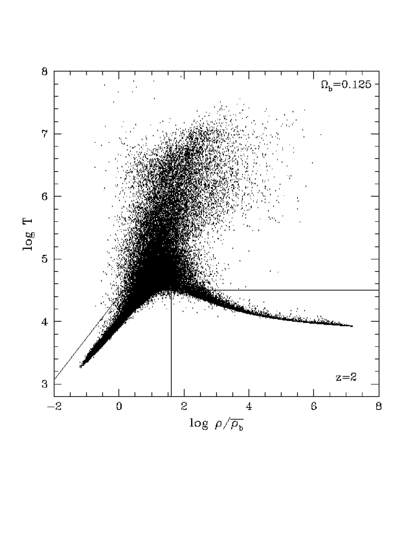
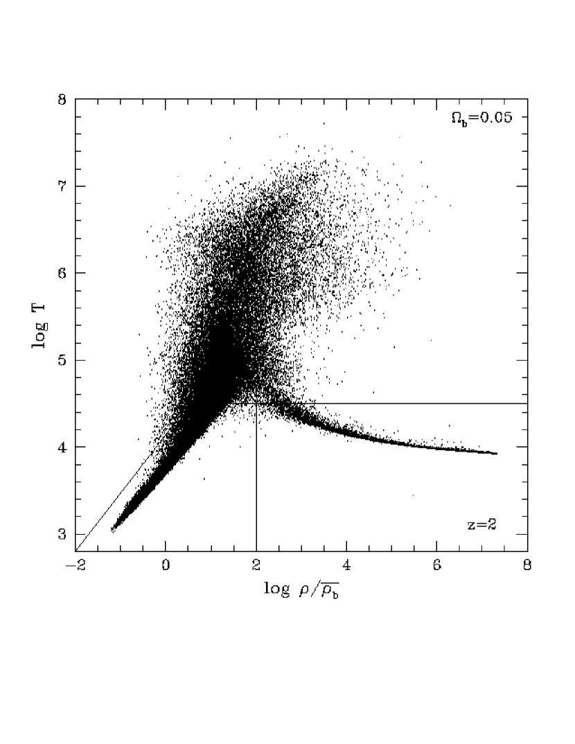
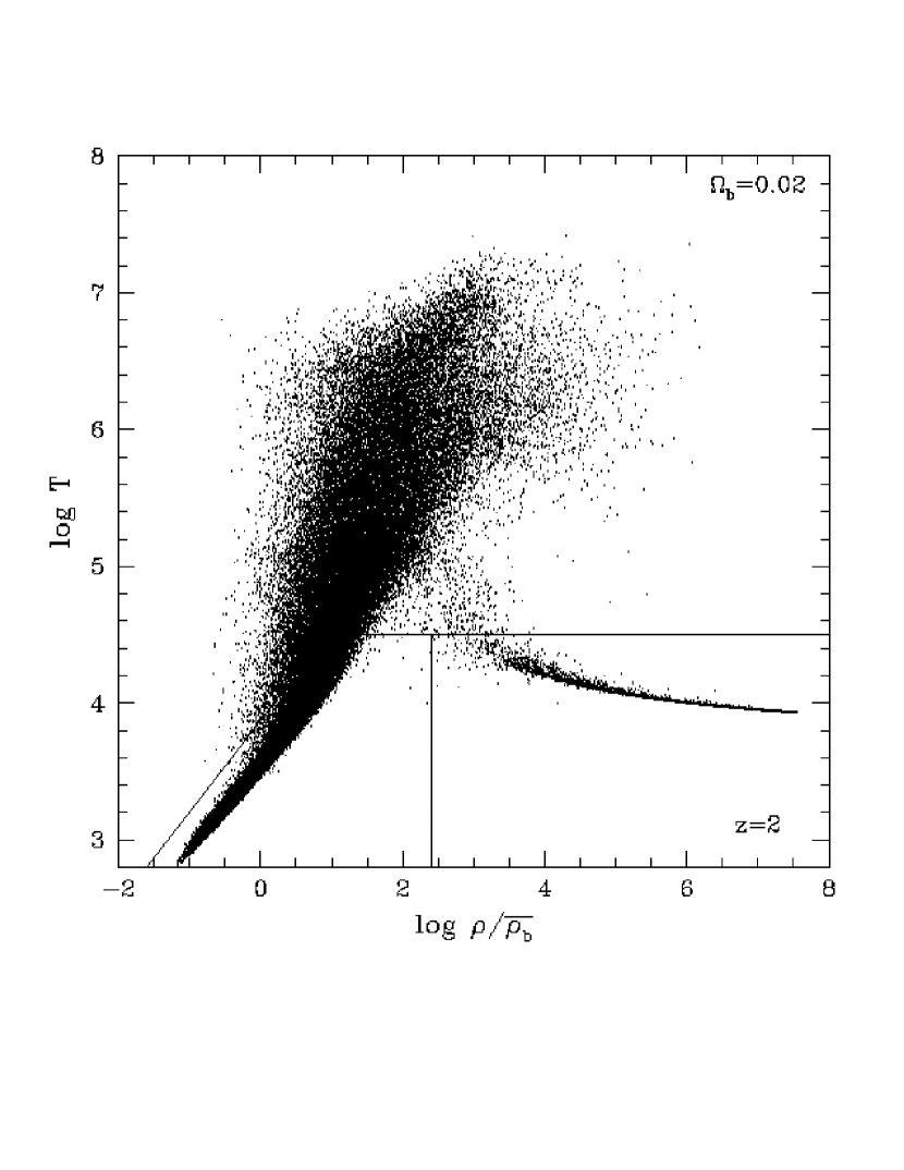
Figure 1: Gas particle density $\rho$ in units of the mean baryon density $\bar{\rho}_{b}$ vs. temperature $T$. The solid lines indicate the borders for gas particles to be considered cool, photoionized, diffuse IGM (lower left box); condensed gas (lower right box); and shocked IGM (upper remainder of panel).

Figure 1 shows the temperature-density distribution for $10^{5}$ randomly selected gas particles in each simulation. We divide $\rho-T$ space into the three major populations according to the prescription in Davé et al. (1999), using the same cutoffs in temperature and physical density:

1. Condensed: ($\log T<4.5$ and $\log\rho/\bar{\rho}_{b}>2$) cold, dense gas associated with galaxies.

2. Diffuse: ($\log T<4.5$ and $\log\rho/\bar{\rho}_{b}<2$ and $\log T<2/3(\log\rho/\bar{\rho}_{b}+2)+2.8$) cool, ionized, diffuse IGM heated by photoionization but able to cool adiabatically.

3. Shocked: (remainder) shocked IGM in the form of shock-heated gas in filaments and halos.

We adopt the term “condensed” to denote gas classified simply by this $\rho-T$ cut to differentiate it from “cold collapsed gas” — part of the cold collapsed gas and stars (CCGS) component presented later on — which is gas that is part of a SKID-identified group (and hence gravitationally self-bound).

Figure 2: Evolution of the mass in the various phases in units of the total baryon mass. The three principal gas phases — diffuse, shocked, and condensed — are given in the first three panels. The fourth panel shows the stellar mass fraction, and the bottommost panel shows condensed gas + stars. The line styles are consistent throughout the paper and are as follows: $\Omega_{b}=0.125$ dotted, $\Omega_{b}=0.05$ solid, and $\Omega_{b}=0.02$ long-dashed. Note that the $y$-axes of the plots differ slightly to enhance differences between models.

Figure 2 compares the mass fraction in each of the three gaseous phases from Figure 1 as a function of redshift. Stellar mass fraction is displayed separately and in combination with condensed gas. Hence, the bottom-left panel is the true measure of condensed matter in the simulation. The line styles denoting the different simulations are the same throughout this paper: $\Omega_{b}=0.125$ dotted, $\Omega_{b}=0.05$ solid, and $\Omega_{b}=0.02$ long-dashed. The higher gas density in high $\Omega_{b}$ cosmologies clearly promotes more aggressive cooling, which in turn enhances star formation activity. The fraction in the diffuse component reflects the original state of the gas and is largely unaffected by variations in global baryon density. Hence, the increased mass in condensed baryons is offset by a deficit in shocked gas. The fact that the condensed and shocked phases establish a balance while leaving the diffuse component unchanged indicates that the gas is shocked in high-density regions physically proximate to the cooling gas, but not in regions that harbor the diffuse component.

Table 1 shows the results of fitting a power law in $\Omega_{b}$ for each of the five components. As one would surmise from Figure 2, the diffuse component exhibits little $\Omega_{b}$ dependence. The baryon dependence of the shocked component is difficult to characterize by a power-law because it varies more strongly when changing $\Omega_{b}$ from 0.02 to 0.05 than from 0.05 to 0.125; in the latter case, the removal of shocked gas to the condensed/stellar phases is partly compensated by a small drop in the diffuse phase. The fractions of baryons in the condensed and stellar phases scale fairly well with $\Omega_{b}$ and can be approximated by power laws that vary approximately as $\Omega_{b}^{1.5}$, with the exact scaling depending on the precise phase and redshift. The errors in the $\chi^{2}$ fit to the exponent are minimal, although it is difficult to assign formal errors to the quantities in Figure 2.

	$\beta$			$\beta(z)$
	$z=2$	$z=3$	$z=4$
Diffuse	0.980	0.980	1.022	minimal dependence
Shocked	0.870	0.890	0.572	no simple dependence
Condensed	1.419	1.539	1.656	$0.12(z-3)+1.54$
Stars	1.534	1.568	1.596	$0.031(z-3)+1.56$
Condensed+Stars	1.484	1.549	1.645	$0.081(z-3)+1.56$
	$z=2$	$z=4$	$z=6$
Star Formation Rate	1.434	1.561	1.714	$0.070(z-3)+1.50$

Table 1: Table of baryonic dependence of global baryon components and other global quantities. The dependence is given as a power law $\Omega_{b}^{\beta}$ shown in columns 2-4. The last column shows the best fit linear dependence of $\beta$ on redshift, centered on redshift $z=3$. The first five lines give the scaling of the mass in the components given in Figure 2. The last line gives the $\Omega_{b}$ scaling of the global star formation rate (Figure 9).

3.2 The Lyman-alpha Forest

Figure 3: Profiles of (top to bottom) transmitted flux, hydrogen neutral fraction, gas overdensity, and temperature, along four lines of sight through each of the three simulations at $z=2$. In each simulation, the intensity of the UV background is adjusted so that the simulation reproduces the observed mean decrement of the LAF. As a result, higher neutral fractions compensate for the lower gas densities in the lower $\Omega_{b}$ models, and the three simulations yield nearly identical LAF spectra.

To study the influence of $\Omega_{b}$ on LAF absorption, we create synthetic spectra using the TIPSY package (Katz & Quinn, 1995), following the algorithm described by Hernquist et al. (1996). If we used the same UV background intensity in all three simulations, then the higher $\Omega_{b}$ runs would have higher gas densities, higher neutral fractions, and a higher mean opacity of the LAF. Instead we follow the by now standard procedure of adjusting the UV background intensity (which is observationally quite uncertain) so that each simulation reproduces the observed mean opacity (see, e.g., Miralda-Escudé et al. 1996; Croft et al. 1997). Table 2 lists the factors by which we must multiply the Haardt & Madau (1996) background intensities to match the Press et al. (1993) values of the LAF mean flux decrement in the three simulations at each redshift. These factors scale roughly as $\Omega_{b}^{1.7}$.

Figure 3 shows spectra and 1-d profiles along four randomly selected lines of sight through the simulations at $z=2$. The gas density profiles (2nd panel up in each case) are virtually identical when computed in units of the mean baryon density. Random lines of sight intersect regions of low to moderate overdensity, where changing the baryon fraction has negligible impact on the density field. Neutral fractions (3rd panel up) are higher for lower $\Omega_{b}$, as they must be to maintain a constant value of the mean flux decrement (which scales roughly with the mean neutral hydrogen density). Temperatures (bottom panel) are higher for higher $\Omega_{b}$ because the higher photoionization rate leads to more rapid heating, while the cooling, which is dominated by adiabatic expansion in these low density regions, stays constant. These higher temperatures are the reason that the required UV background intensity scales as $\Omega_{b}^{1.7}$ rather than $\Omega_{b}^{2}$ as one might naively expect. Higher temperatures reduce the recombination coefficient, so the neutral fraction at fixed photoionization rate does not grow as fast as $\Omega_{b}$.

The top panels in Figure 3 show the synthetic spectra themselves, and they are virtually indistinguishable for the three different $\Omega_{b}$ values. Because the gas overdensity structure is nearly independent of $\Omega_{b}$, normalizing the UV background to match a fixed mean decrement makes the spectra match point by point, with only a minor difference caused by differences in thermal broadening. Figure 3 thus provides strong backing for the standard practice of scaling LAF spectra derived from hydrodynamic simulations. When gas temperatures are set by the interplay between photoionization heating and adiabatic cooling, as they are here, then the parameter combination constrained by the observed mean opacity scales as $\Gamma/\Omega_{b}^{1.7}$, where $\Gamma$ is the HI photoionization rate.

$\Omega_{b}$	$z=2$	$z=4$	$z=4$
0.125	1.90	1.78	5.34
0.05	0.40	0.40	1.20
0.02	0.08	0.09	0.27

Table 2: Table of factors by which the Haardt & Madau (1996) UV background intensity must be multiplied in order for the mean opacity of the simulation volume to match Press et al. (1993) values.

3.3 Damped Ly$\alpha$ and Lyman Limit Systems

Figure 4: Effects of $\Omega_{b}$ on damped Ly$\alpha$ absorber and Lyman limit incidence $n(z)$. We evaluate all models at the same redshifts $z=2,3,4$ but plot them with slightly offset $z$ values for greater clarity. Because the simulations only resolve absorbers in halos with $v_{c}\geq 100$ km s^-1, they are expected to underestimate the true incidence of absorption, perhaps by a large factor (see GKHW). These are plotted against damped Ly$\alpha$ absorber observational values from Storrie-Lombardi & Wolfe (2000) and Lyman limit observational values from Storrie-Lombardi et al. (1994). The observations are shown with $1\sigma$ (solid) and $2\sigma$ (dashed) error bars. Error bars on the simulation points denote the 68.3% confidence limit.

We measure the incidence $n(z)$ of damped Ly$\alpha$ (DLA) and Lyman limit (LL) systems in each simulation using the method described in GKHW. By “incidence” we mean the number of systems with $N_{\rm HI}\geq 10^{20.3}\;{\rm cm}^{-2}$ (DLA) or $N_{\rm HI}\geq 10^{17.2}\;{\rm cm}^{-2}$ (LL) intercepted along a line of sight per unit redshift. Although our simulations only resolve halos with virial radius circular velocities $v_{c}\mathrel{\hbox{\raise 2.15277pt\hbox{$>$}\hbox to0.0pt{\hss\lower 2.15277pt\hbox{$\sim$}}}}100$ km s^-1, GKHW find that a significant fraction, possibly even the majority, of the DLA and LL incidence arises in halos less than this cutoff. Consequently, in comparing our simulated $n(z)$ to observational values in Figure 4, we would expect our results to be below what is observed and serve as lower limits. However, given that all three simulations have the same mass resolution, we can compare the simulations against one another to understand how DLA and LL incidence is affected by $\Omega_{b}$.

GKHW and Gardner et al. (1997) demonstrated that the cross-section of halos harboring DLA and LL absorbers was a complex function of halo mass, interaction history, and cooling time. Specifically, absorbers that are able to cool more quickly tend to have more mass in cooled neutral gas but also smaller cross-sections as the gas tends to collapse more tightly. The competing effect that helps determine the halo absorption cross-section is that higher mass halos tend to harbor more absorbers, thus increasing the overall absorption cross-section with mass. The incidence of DLA and LL systems, however, follows the intuitive expectation that a higher $\Omega_{b}$ means more absorbers. If we examine the results on a halo by halo basis (not shown) we find that, in general, the scaling in Figure 4 results from halos of all masses having uniformly larger absorption cross-sections in higher $\Omega_{b}$ models. Hence, although the complex link between gas mass and DLA/LL cross-section need not have yielded an intuitive relationship between cross-section and $\Omega_{b}$, DLA and LL incidence does appear to scale in a relatively simple manner with the universal baryon fraction.

3.4 Baryonic Behavior Within Dark Matter Halos

Figure 5: Effect of $\Omega_{b}$ on halo baryon fraction and cooling fraction at redshift $z=2$. Each data point represents a specific halo which was identified in the two simulations labeled on the $x$ and $y$ axes. The upper panels compare the baryon fraction of a FOF-identified halo in each simulation, normalized to the Universal value, $\Omega_{b}/\Omega_{m}$. The lower panels plot the fraction of cold collapsed gas and stars (CCGS) with respect to the total baryonic content of the halo. The solid line indicates the locus of no dependence on cosmic baryon abundance.

We now examine the behavior of baryons within collapsed objects, specifically groups which have been identified with the FOF algorithm and are above the mass resolution cutoff. Cold collapsed gas and stars (CCGS) in each halo are identified using SKID as detailed in section 2.1. Figure 5 compares the baryonic fraction and the fraction of baryons in CCGS in each of the simulations. Given that the simulations have the same total mass and were run from exactly the same initial waves, it is simple to identify the corresponding halos in each simulation. Each point in Figure 5 represents the same halo identified in all three simulations and matched based on its position. Looking at the top panels, we notice that at $z=2$ the baryonic fraction of halos normalized to the baryonic fraction of the Universe as a whole is insensitive to $\Omega_{b}$ for $\Omega_{b}\geq 0.05$, i.e. the baryonic fraction of a halo just scales linearly with $\Omega_{b}$. Interestingly, the average baryonic fraction of halos in these models is greater than the universal fraction. Thus, somehow baryons are managing to collapse more readily than the dark matter, indicating that collapse beyond the boundaries of dark matter halos is not purely gravitationally driven. We examine this topic in Gardner et al.  (2001b). The $\Omega_{b}=0.02$ model, however, does not have an overabundance of baryons, showing that the process is nonlinear below some mass or density threshold.

Larger numbers of baryons within dark matter halos do uniformly lead to enhanced cooling and collapse, as evidenced by the lower panels in Figure 5. Hence, more baryons in the Universe cause a greater fraction of them to become galactic CCGS. We will examine the effect of this on galaxy properties in the next section.

Figure 6: Similar to Figure 5, but compares total FOF-identified halo mass in the form of CCGS (top) and stars (middle), as well as the total SFR in each halo. All plots are for redshift $z=2$. The solid line shows 1-to-1 correspondence while the long-dashed line is offset by the ratio of $\Omega_{b}$.

Next, let us turn our attention to the CCGS. The upper panel of Figure 6 is consistent with Figure 5 in that both sets of points lie above the dashed line, indicating a greater than linear dependence of CCGS mass on $\Omega_{b}$. The scaling goes as $\Omega_{b}^{1.23\pm 0.02}$ in the redshift range $2\leq z\leq 4$ (only the $z=2$ data are shown in Figure 6). More CCGS also produces more stars (as opposed to just cold collapsed gas), as evidenced by the middle panels. Stellar mass scales similarly to CCGS as $\Omega_{b}^{1.33\pm 0.3}$. Both scalings are listed in Table 3.

Most likely, there is a critical gas mass required in the central regions of our simulated galaxies for star formation to occur efficiently. The horizontal features at low halo stellar masses indicate that star formation is severely damped at these masses for lower $\Omega_{b}$ when compared to their higher $\Omega_{b}$ counterparts. All of the halos plotted in Figure 6 are above our resolution limit of 64 dark matter particles. Even so, GKHW find similar behavior when comparing higher resolution simulations to lower resolution ones of the same cosmology. Consequently, this is most likely a resolution effect. Therefore, the scalings in $\Omega_{b}$ reported above are calculated using only those points in the higher mass regions that are well approximated by a power law (for the top and middle panels for masses greater than $10^{10}M_{\odot}$; for the bottom panels for star formation rates greater than 0.85 M_⊙ yr^-1). One may note that the scalings given here are different from those in Section 3.1. Here we include only baryons in dark matter halos, whereas before we examined all baryons. We believe that the steeper scaling of the global quantities could also be due to a resolution artifact. Halos at the limit of our resolution cross a critical threshold when the gas particles are more massive, i.e. higher $\Omega_{b}$, but do not cross that threshold when the gas particles are less massive, i.e. lower $\Omega_{b}$. Remember that the number of gas particles is the same for all the simulations; we change $\Omega_{b}$ by altering the gas particle mass.

Although the star formation rate is not shown for redshifts $z=3,4$, the $\Omega_{b}$ scaling does depend strongly on redshift, going as $\Omega_{b}^{1.2}$, $\Omega_{b}^{1.1}$, and $\Omega_{b}^{1.5}$ for redshifts 2, 3, and 4, respectively. Owing to the large scatter, it is difficult to achieve the precision of the stellar and CCGS mass measurements. However, it is clear that the star formation rate scales beyond simple linearity. Given that that the relation is close to linear for $z\leq 3$, the increased stellar mass in the middle panels most likely comes from a higher star formation rate at earlier redshifts.

The careful reader will note that there are points below $10^{9}M_{\odot}$ for the $\Omega_{b}=0.05$ run in the left panel in the middle row but not in the right panel. This is because the halos in the $\Omega_{b}=0.05$ run with such a low stellar mass have no SKID-identifiable groups at all in the $\Omega_{b}=0.02$ run and hence are not included in the $\Omega_{b}=0.05$ vs. $\Omega_{b}=0.02$ plot. Since gas particle mass scales with $\Omega_{b}$, we would expect to detect SKID groups in both simulations if stellar mass scaled simply with $\Omega_{b}$. The fact that there are no SKID groups in the low $\Omega_{b}$ halos that have SKID groups at higher baryon abundance again indicates a steep $\Omega_{b}$ dependence.

3.5 Galactic Gas and Star Formation Rate

Figure 7: Effect of $\Omega_{b}$ on galaxy stellar and total mass. The lines indicate the cumulative mass function of stars (left panels) or gas + stars (right panels) in SKID-identified groups, i.e. galaxies, in each of the three simulations.

Figure 8: Effect of $\Omega_{b}$ on galaxy star formation rate. The lines indicate the cumulative number density of SKID-identified groups with a star formation rate greater than the $x$-axis value.

Figure 9: Total star formation in resolved halos for each $\Omega_{b}$ expressed as a comoving density and plotted in log space. The straight long-dashed line is the present mass density of metals divided by present age of the Universe, taken from Madau et al (1996).

In this section, we concentrate on the effect of universal baryon fraction on galaxies. In contrast to the previous sections, here we consider SKID-identified groups of gas and stars — i.e. galaxies in our simulations — irrespective of their parent FOF-identified parent halos. We keep plotted values in units unnormalized to the universal fraction to more easily relate them to observables. Figure 7 plots the cumulative comoving number density of galaxies $n(M)$ with mass $>M_{*}$ in stars or $>M_{\rm gal}$ in CCGS, while Figure 8 plots the cumulative number of galaxies with at least a given star formation rate (SFR). Given that the halo mass function is essentially identical in all three simulations, the plots indicate a direct correspondence between $\Omega_{b}$ and typical galaxy gas, stellar mass and star formation rate. Figure 9 gives the total star formation rate in resolved galaxies as a function of redshift for all three simulations. Note that this does not include star formation in galaxies with $v_{c}\mathrel{\hbox{\raise 2.15277pt\hbox{$<$}\hbox to0.0pt{\hss\lower 2.15277pt\hbox{$\sim$}}}}100$ km s^-1, which make a significant contribution to the total star formation rate at high redshift. The global SFR is a strong function of the universal baryon fraction and is well approximated by a power law. The detailed scaling is given in Table 1 and goes roughly as $\Omega_{b}^{1.5}$ with modest redshift dependencies.

	$\beta$
	$z=2$	$z=3$	$z=4$
Star Formation Rate	1.2	1.1	1.5
CCGS	$1.23\pm 0.02$
Stars	$1.33\pm 0.03$

Table 3: Table of baryonic dependence, $\Omega_{b}^{\beta}$, of CCGS, stars, and star formation rate inside dark matter halos individually identified in each simulation, as given in Figure 6.

4 Summary

We present an analysis of the effects of $\Omega_{b}$ on a broad range of measurable properties in our simulations. Our results our summarized in Tables 1–3, where we present the power law scaling of the quantities with $\Omega_{b}$. The amount of baryonic material scales linearly with $\Omega_{b}$. The cooling rate scales as $\Omega_{b}^{2}$, so one might have expected the scalings of quantities related to the condensed galactic material to scale with a power law index between one and two, and that is just what we find.

Dividing the total gas in the each simulation into three phases, based on density and temperature, we find that the primordial diffuse phase remains largely unaffected by changes in $\Omega_{b}$. Shocked and condensed gas, however, exchange abundances with condensed gas being more prevalent in higher $\Omega_{b}$ universes while less mass is contained in the shocked phase. This is consistent with Murali et al. (2001) who find that galaxies gain mass mostly through the smooth accretion of cooling gas and not through merging. A general theme of our results is that higher $\Omega_{b}$ promotes increased gas cooling. The mass in condensed gas and stars is well described by a power law in $\Omega_{b}$ of greater than linear scaling, as detailed in Table 1. Dark matter halos in higher $\Omega_{b}$ cosmologies contain more than their fair share of both cold collapsed gas and stars, meaning galaxies also tend to be more massive at $2\leq z\leq 4$ in these universes. A larger fraction of galaxies in high $\Omega_{b}$ models have high rates of star formation, and the universal star formation rate is also greater. Cold collapsed gas and stars as well as stellar mass alone scale superlinearly as given in Table 3.

Because it probes gas in the diffuse phase, the LAF is insensitive to the value of $\Omega_{b}$ provided that the UV background intensity is adjusted to reproduce the observed mean opacity of the forest. The required UV background intensity scales approximately as $\Omega_{b}^{1.7}$, and diffuse gas in a higher $\Omega_{b}$ model is slightly hotter because of the higher photoionization rate. The gas overdensity field is essentially independent of $\Omega_{b}$ in diffuse regions, and higher neutral fractions compensate for lower gas densities when $\Omega_{b}$ is low, so synthetic spectra are virtually identical for different values of $\Omega_{b}$. These results support the standard practice of scaling LAF spectra from hydrodynamic simulations to match the observed mean opacity.

As one would intuitively expect, models with higher $\Omega_{b}$ have increased DLA and LL absorption. The $\Omega_{b}$ dependence is much stronger for DLA absorption than for LL absorption, and it is somewhat stronger at $z=2-3$ than at $z=4$. Our simulations only resolve baryon concentrations in halos with $v_{c}\geq 100{\rm km}\;{\rm s}^{-1}$, and they therefore underestimate the total incidence of DLA and LL absorption. However, the trend of increased absorption with increasing $\Omega_{b}$ holds on a halo-by-halo basis within the mass range that we do resolve, so we expect that it would continue to apply to the absorption in all halos.

Taken together, our results imply a relative simple picture of the influence of $\Omega_{b}$ on high-redshift structure. The amount of gas in the diffuse phase is essentially unaffected by changes in $\Omega_{b}$, and the LAF absorption produced by this gas is unchanged if the UV background is adjusted to keep the mean opacity fixed. The increased cooling in models with high $\Omega_{b}$ shifts gas from the shocked phase to the condensed phase, increasing the stellar and gas masses of galaxies, the rates of star formation, and the amount of high column density absorption. While the $\Omega_{b}$-scalings of these quantities that are listed in Table 1 are not guaranteed to hold in other cosmologies or other ranges of redshift and galaxy mass, they provide a best guess for how to scale the predictions of hydrodynamic simulations to alternative values of $\Omega_{b}$. If the current consensus on the value of $\Omega_{b}$ survives improvements in the observations, then the remaining uncertainties in $\Omega_{b}$ will contribute relatively little uncertainty to predictions of high-redshift structure.

References

- Barnes & Hut (1986) Barnes, J.E. & Hut, P. 1986, Nature, 324, 446
- Burles & Tytler (1998ab) Burles, S., & Tytler, D. 1998a, ApJ, 499, 699
- Burles & Tytler (1998) Burles, S., & Tytler, D. 1998b, ApJ, 507, 732
- Croft et al. (1997) Croft, R.A.C., Weinberg, D.H., Katz, N., Hernquist, L., 1997, ApJ, 488, 532
- D’Odorico et al. (2001) D’Odorico, S., Dessauges-Zavadsky, M., & Molaro, P. 2001, A&A, in press, astro-ph/0102162
- Davé et al. (1999) Davé, R., Hernquist, L., Katz, N., & Weinberg, D.H. 1999, ApJ, 511, 521.
- Gardner et al. (2001a) Gardner, J. P., Katz, N., Hernquist, L., & Weinberg, D. H. 2000a, ApJ, in press, astro-ph/9911343 (GKHW)
- Gardner et al. (2001b) Gardner, J. P., Katz, N., Weinberg, D. H., & Hernquist, L. 2000b, in preparation
- Gardner et al. (1997) Gardner, J. P., Katz, N., Hernquist, L., & Weinberg, D. H. 1997, ApJ, 484, 31
- Gingold & Monaghan (1977) Gingold, R.A. & Monaghan, J.J. 1977, MNRAS, 181, 375
- Haardt & Madau (1996) Haardt F., & Madau P. 1996, ApJ, 461, 20
- Hernquist (1987) Hernquist, L. 1987, ApJS, 64, 715
- Hernquist & Katz (1989) Hernquist, L. & Katz, N. 1989, ApJS, 70, 419
- Hernquist et al. (1996) Hernquist, L., Katz, N., Weinberg, D.H. & Miralda-Escudé, J. 1996, ApJ, 457, L51
- Jaffe et al. (2001) Jaffee, A.H., et al. 2001, Phys. Rev. Lett., 86, 3475
- Katz, Hernquist & Weinberg (1999) Katz, N., Hernquist, L., & Weinberg D.H. 1999, ApJ in press, astro-ph/9806257
- Katz & Quinn (1995) Katz, N., & Quinn, T. 1995, TIPSY manual
- Katz, Weinberg, & Hernquist (1996) Katz, N., Weinberg D.H., & Hernquist, L. 1996, ApJS, 105, 19 (KWH)
- Kurki-Suonio & Sihvola (2001) Kurki-Suonio, H. & Sihvola, E. 2001, Phys. Rev. D, 63, astro-ph/0011544
- Lange et al. (2000) Lange, A. E., and 31 colleagues 2000, astro-ph/0005004
- Lucy (1977) Lucy, L. 1977, AJ, 82, 1013
- Miralda-Escudé et al. (1996) Miralda-Escudé J., Cen R., Ostriker, J.P., & Rauch, M. 1996, ApJ, 471, 582
- Murali et al. (2001) Murali, C., Katz, N., Hernquist, L., Weinberg, D. H. & Daveé, R. 2001, astro-ph/0106282
- Netterfield et al. (2001) Netterfield, C. B. et al. 2001, ApJ, submitted, astro-ph/0004460
- O’Meara et al. (2001) O’Meara, J.M., Tytler, D., Kirkman, D., Suzuki, N., Prochaska, J.X., Lubin, D., & Wolfe, A.M. 2001, ApJ, in press, astro-ph/0011179
- Padmanabhan & Sethi (2000) Padmanabhan, T., & Sethi, S.K. 2000, ApJ, submitted, astro-ph/0010309
- Pettini & Bowen (2001) Pettini, M., & Bowen, D.V. 2001, ApJ, submitted, astro-ph/0104474
- Press, Rybicki, & Schneider (1993) Press, W. H., Rybicki, G. B., & Schneider, D. P. 1993, ApJ, 414, 64
- Pryke et al. (2001) Pryke, C., Halverson, N. W., Leitch, E. M., Kovac, J., Carlstrom, J. E., Holzapfel, W. L., & Dragovan, M. 2001, ApJ, submitted, astro-ph/0004490
- Rugers & Hogan (1996) Rugers, M. & Hogan, C. J. 1996, ApJ, 459, L1
- Songaila, Cowie, Hogan & Rugers (1994) Songaila, A., Cowie, L. L., Hogan, C. J. & Rugers, M. 1994, Nature, 368, 599
- Stadel et al. (2000) Stadel, J., Katz, N., Weinberg, D.H., & Hernquist, L. 2000, in preparation
- Storrie-Lombardi et al. (1996) Storrie-Lombardi, L.J., Irwin, M.J., & McMahon, R.G. 1996, MNRAS, 282, 1330
- Storrie-Lombardi et al. (1994) Storrie-Lombardi, L.J., McMahon, R.G., Irwin, M.J., & Hazard, C. 1994, ApJ, 427, L13
- Storrie-Lombardi & Wolfe (2000) Storrie-Lombardi, L. J. & Wolfe, A. M. 2000, ApJ, 543, 552
- Tytler et al. (2000) Tytler, D., O’Meara, J.M., Suzuki, N., & Lubin, D. 2000, Phys. Scr, in press, astro-ph/0001318
- Webb et al. (1997) Webb, J. K., Carswell, R. F., Lanzetta, K. M., Ferlet, R., Lemoine, M., Vidal-Madjar, A., & Bowen, D. V. 1997, Nature, 388, 250