Sub-mm Galaxies in Cosmological Simulations

Abstract

We study the predicted sub-millimeter emission from massive galaxies in a $\Lambda$-dominated cold dark matter universe, using hydrodynamic cosmological simulations. Assuming that most of the emission from newly formed stars is absorbed and reradiated in the rest-frame far-infrared, we calculate the number of galaxies that would be detected in sub-mm surveys conducted with SCUBA. The predicted number counts are strongly dependent on the assumed dust temperature and emissivity law. With plausible choices for parameters of the far-IR spectral energy distribution (e.g., $T=35\,\mbox{K}$, $\beta=1.0$), the simulation predictions reproduce the observed number counts above $\sim 1\,\mbox{mJy}$. The sources have a broad redshift distribution with median $z\approx 2$, in reasonable agreement with current observational constraints. However, the predicted count distribution may be too steep at the faint end, and the fraction of low redshift objects may be larger than observed.

In this physical model of the sub-mm galaxy population, the objects detected in existing surveys consist mainly of massive galaxies (several $M_{\ast}$) forming stars fairly steadily over timescales $\sim 10^{8}-10^{9}$ years, at moderate rates $\sim 100\,M_{\sun}\,\mbox{yr}^{-1}$. The typical descendants of these sub-mm sources are even more massive galaxies, with old stellar populations, found primarily in dense environments. While the resolution of our simulations is not sufficient to determine galaxy morphologies, these properties support the proposed identification of sub-mm sources with massive ellipticals in the process of formation. The most robust and distinctive prediction of this model, stemming directly from the long timescale and correspondingly moderate rate of star formation, is that the far-IR SEDs of SCUBA sources have a relatively high 850 µm luminosity for a given bolometric luminosity. Other model predictions can be tested with future studies of the redshift distribution, rest-frame UV/optical properties, and angular and redshift-space clustering of sub-mm galaxies.

1 INTRODUCTION

The observation of galaxies in the sub-millimeter has become a crucial area of astronomy since the installation of the SCUBA camera on the JCMT (the field is reviewed by Blain et al. 1999a). Because emission from dust in galaxies rises sharply up to a peak at $\sim\!100$ µm, sub-mm observations preferentially detect high-redshift galaxies. While it was known from optical/near-IR observations that the cosmic star formation rate increases steeply with redshift up to at least $z\approx 2$ (Madau, Pozzetti & Dickinson, 1998), measurement of the extragalactic background with FIRAS (Fixsen et al., 1998) suggested that still more of the high-redshift star formation is hidden in the optical. The first SCUBA surveys (Smail, Ivison & Blain, 1997; Hughes et al., 1998; Barger et al., 1998) immediately showed that a large fraction of this hidden star formation takes place in extremely luminous systems, with star formation rates of $\gtrsim 100\,M_{\sun}\,\mbox{yr}^{-1}$.

Many authors have conjectured that the objects dominating the SCUBA surveys are elliptical galaxies or spheroidal components of disk galaxies in the process of formation. The analogy to low-redshift galaxies that are similarly bright in the far-infrared (FIR) suggests that they may be experiencing bursts of star formation due to major mergers. Although the surveys are increasing in depth and quantity, the low resolution, small fields, and large noise of the SCUBA maps compared to optical surveys leads to many systematic uncertainties that are still poorly quantified. Optical counterparts of the SCUBA sources are still difficult to identify, and there are very few detections in the FIR at wavelengths other than 850 µm. As a result, vigorous debates continue about the redshift distribution and star formation rates of the sources, the fraction of their energy supplied by AGN and star formation, their connection to other populations such as the Lyman break galaxies, and the contribution of these sources to the cosmic star formation rate (Lilly et al., 1999; Blain et al., 1999b; Adelberger & Steidel, 2000; Eales et al., 2000).

Comparison of these sub-millimeter observations to current theories of galaxy formation is clearly an important task. Modeling of the SCUBA population has so far been done in a phenomenological manner. For example, Blain et al. (1999b) and Blain et al. (1999c) showed there must be rapid luminosity evolution in the infrared galaxy luminosity function to reproduce the observed counts and sub-mm background. Guiderdoni et al. (1998) found that matching the counts within their semi-analytic model of galaxy formation required the ad hoc addition of a component of starbursting systems whose numbers increase rapidly with redshift. Artificial catalogs of sub-mm sources have also been constructed using Poisson-distributed sources (Eales et al., 2000) or large-scale dark matter simulations (Hughes & Gaztañaga, 2000), to aid in measurement of observational systematics. While useful, such catalogs do not bring one any closer to a physical understanding of these sources.

In this paper, we use numerical N-body/hydrodynamical simulations to study the sub-mm galaxy population. This paper follows several others devoted to the galaxy population in our simulations (Katz, Hernquist, & Weinberg, 1999; Weinberg et al., 1999; Davé et al., 1999b; Weinberg, Hernquist, & Katz, 2000). These papers showed that the optically detected Lyman-break galaxies at $z\approx 3$ are a natural consequence of CDM models, assuming reasonable amounts of dust extinction. They focused on the dependence of the galaxy abundance on the assumed cosmology and the clustering of these sources. This paper concentrates on the correspondence between the galaxies in our simulation and the bright sub-mm sources detectable with SCUBA. We restrict the study to a single cosmology, the currently favored $\Lambda$-dominated cold dark matter (LCDM) model. We rely primarily on a single simulation of a large volume but only moderate mass resolution, which is well suited to a statistical study of the bright, rare sources. We defer a detailed discussion of fainter sources, the FIR background, and the relation between the sub-mm and UV/optical populations to a future paper using higher resolution, smaller volume simulations that are currently underway (Fardal et al., 2001).

We describe our numerical simulations in § 2, where we also discuss the resulting galaxy population and examine the effects of numerical resolution. In § 3, we describe our recipe for calculating the sub-mm fluxes. Our method ignores the detailed physics of dust absorption and emission, opting instead for simple, parameterized models motivated by observations. In § 4, we constrain these parameters by requiring the simulated galaxy population to match the counts at $\sim\!3\,\mbox{mJy}$. We compare the resulting flux and redshift distributions to observations, arguing that the sub-mm population can be reproduced in our simulations for plausible assumptions about dust emission. In § 5, we examine the physical properties of the simulated galaxies that correspond to SCUBA sources. Section 6 discusses our confrontation of the simulations with observations and presents our conclusions.

2 SIMULATING THE GALAXY POPULATION

Our simulations are performed with the N-body/hydro code Parallel TreeSPH. This code follows both the gas and the dark matter with discrete particles, using spline kernel interpolation to smooth the gas quantities over a compact set of particles. The code is described elsewhere in detail (Hernquist & Katz, 1989; Katz, Weinberg, & Hernquist, 1996; Davé, Dubinski, & Hernquist, 1997). Simulations with this code have been successful in reproducing the observed clustering pattern and evolutionary trends of galaxies (Katz, Hernquist, & Weinberg, 1999; Weinberg, Hernquist, & Katz, 2000), as well as phenomena such as the Lyman-$\alpha$ forest (Hernquist et al., 1996; Davé et al., 1999a), and the abundance of higher-column density systems, including Lyman-limit and damped Lyman-$\alpha$ absorbers (e.g. Gardner et al. 1997a,b; 2000).

Star formation in this simulation is determined heuristically using local physical properties of the gas. For star formation to take place within a gas particle, the gas must be cold ($T<3\times 10^{4}\,\mbox{K}$), dense ($\rho_{H}>0.1\,\mbox{cm}^{-3}$ and overdensity $\rho_{g}/{\bar{\rho}_{g}}>55.7$), converging, and Jeans unstable. The star formation timescale is determined by the local cooling and dynamical timescales, and because the star formation rate is an increasing function of gas density, the star formation rate in a simulated galaxy is governed mainly by the rate at which gas condenses and cools onto the central object (see Katz, Weinberg, & Hernquist 1996 for details of the algorithm and Weinberg, Hernquist, & Katz 2000 for further discussion). We identify galaxies in the simulations at the sites of local baryonic density maxima, using the program SKID. SKID finds galaxies by first determining the smoothed density field, then moving particles upward along the gradient of the density field. We define the galaxy to be the set of particles that aggregate at a particular density peak after removing particles that do not satisfy a negative energy binding criterion. To be included in a galaxy, gas particles must also have a temperature $T<3\times 10^{4}\,\mbox{K}$ and and a density $\rho>10^{3}\Omega_{b}$, i.e. we consider only the cold gas and stars, the material that comprises the bulk of the matter in the central, visible regions of galaxies. Adding up the star formation rates for the individual particles in the galaxy gives the total star formation rate for that galaxy. Emission from active galactic nuclei or quasars is not included in the simulation.

Properties of the simulated galaxies are described in Weinberg et al. (1999) and Weinberg, Hernquist, & Katz (2000). Galaxies in the simulations form with a 2-phase gas structure: a central glob of gas at $\sim\!10^{4}\,\mbox{K}$ that forms stars, surrounded by hotter gas at $\sim\!10^{6}\,\mbox{K}$. Galaxies with luminosities comparable to the Lyman break galaxies form in abundance even at $z>5$. The clustering of these high-redshift galaxies is highly biased relative to the mass, in accordance with observations (Katz, Hernquist, & Weinberg, 1999). The star formation rates in the simulated galaxies are relatively steady on timescales of 200 Myr.

Comparing simulations of different resolutions and volumes, we find that there is a regime in which the galaxy properties are robust to changing these numerical parameters. The criterion for the low-mass end of this regime is that the galaxy should have $\sim\!64$ cool gas or star particles. At the high-mass end, the volume should be large enough to allow halos of a given size to form in significant numbers. This latter criterion is less easy to quantify (as it is affected not only by Poisson statistics but also by the exclusion of long-wavelength modes in finite boxes), but it can be seen empirically as an upper cutoff in the mass function that depends on the box size. The star formation rates of the galaxies are strongly correlated with the galaxy masses, especially at high redshift. Hence, the star formation rate also has a characteristic resolution limit, though it is not as sharply defined as the mass limit. Because of the restricted range of halo masses, any one simulation represents only a portion of the total star formation.

We refer to the main simulation used in this paper as the L50/144 simulation. This simulation is tuned to study the evolution of large ($L\gtrsim L_{\ast}/4$) galaxies down to $z=0$. It has $144^{3}$ particles in each of the gas and dark matter components, and models a periodic cube that is $50h^{-1}$ comoving  Mpc on a side. This gives us a baryonic mass resolution of $5.4\times 10^{10}\,M_{\sun}$ (based on the 64-particle limit above), and a spatial resolution of $7.0h^{-1}$ comoving  kpc (equivalent Plummer softening). We assume a $\Lambda$ dominated cold dark matter cosmological model with $\Omega_{m}=0.4$, $\Omega_{\Lambda}=0.6$, $h\equiv H_{0}/(100\,\mbox{km}\,\mbox{s}^{-1}\,\mbox{Mpc}^{-1})=0.65$ and a primeval spectral index $n=0.93$. With the tensor mode contribution, normalizing to COBE using CMBFAST (Seljak & Zaldarriaga, 1996; Zaldarriaga, Seljak, & Bertschinger, 1998) implies a normalization $\sigma_{8}=0.8$, which provides a good match to cluster abundances (White, Efstathiou, & Frenk, 1993). We use the Hu & Sugiyama (1996) formulation of the transfer function. We adopt a baryonic density $\Omega_{b}=0.02\,h^{-2}$ consistent with the deuterium abundance in high-redshift Lyman-limit systems (Burles & Tytler, 1997, 1998), and the opacity of the high-redshift Lyman-$\alpha$ forest (e.g. Rauch et al. 1997).

For describing the faintest sub-mm sources and for computing the FIR background, the L50/144 simulation has insufficient resolution. We are conducting a suite of simulations with the same cosmology as above, but with different resolutions and box sizes to test the sensitivity of our results to these parameters. In this paper, we supplement the results of the L50/144 simulation with those of two additional simulations. L11/64 uses $64^{3}$ particles in an $11.1h^{-1}\,\mbox{Mpc}$ volume evolved to $z=0$; this simulation has a mass resolution of $6.8\times 10^{9}\,M_{\sun}$ and a spatial resolution of $3.5h^{-1}$ comoving  kpc. The other simulation, L11/128, uses $128^{3}$ particles in an $11.1h^{-1}\,\mbox{kpc}$ volume evolved to $z=3$; this simulation has a mass resolution of $8.5\times 10^{8}\,M_{\sun}$ and a spatial resolution of $1.75h^{-1}$ comoving  Mpc. When combined, these simulations give consistent results for the number density of galaxies with different star formation rates at high redshift (see Weinberg et al. 1999).

Although we will focus mainly on the bright sources that should be adequately represented in the L50/144 simulation, for some purposes we want to consider the contribution of lower mass systems. To do so, we fit the star formation rate (SFR) distribution across the L144/50, L64/11, and (at $z>3$) L128/11 simulations, using a Schechter (1976) function, which turns out to be a reasonable fit:

$$\frac{dn}{d(\mbox{\it SFR})} = \frac{\phi_{\ast}}{\mbox{\it SFR}_{\ast}}(\mbox{\it SFR}/\mbox{\it SFR}_{\ast})^{\alpha_{s}}e^{-\mbox{\it SFR}/\mbox{\it SFR}_{\ast}}\;,$$

$$\mbox{\it SFR}_{\ast} = \mbox{\it SFR}_{\ast}^{0}(1+z)^{\delta_{s}+\gamma_{s}\ln(1+z)}\;,$$ (1)

with $\phi_{\ast}=6.49\times 10^{-3}\,h^{3}\,\mbox{Mpc}^{-3}\mbox{dex}^{-1}$, $\alpha_{s}=-1.96$, $\mbox{\it SFR}_{\ast}^{0}=33.9\,M_{\sun}\,\mbox{yr}^{-1}$, $\delta_{s}=2.63$, and $\gamma_{s}=-1.04$. This fit is in good agreement with the L50/144 simulation in its valid range of star formation rates. We choose a lower cutoff on the SFR to correspond to the completeness limit of the L11/64 simulation, which roughly equates to ${\it SFR}_{\it min}=1.4\,(1+z)^{1.6}\,M_{\sun}\,\mbox{yr}^{-1}$. We then generate an artificial high-resolution “galaxy” population from these fits. Naturally, this artificial sample can be used only as an indicator of the results expected from a higher-resolution, large-volume simulation. It also cannot be used to study the spatial distribution or merger history of the galaxies. Further discussion of our fitting methods and results with a fuller set of simulations will be presented in Fardal et al. (2001).

The star formation rates in the simulations are the foundation of this paper, so we review here what we already know or suspect about the validity of these rates. For the cosmological model considered here, the simulations reproduce the observed density of Lyman-break galaxies given a reasonable amount of extinction (Weinberg, Hernquist, & Katz, 2000; Davé et al., 1999b). The cosmic star formation rate rises from $z=0$ back to $z\approx 2$–3 and then falls off, though we are still testing the sensitivity of the high-redshift decline to resolution (Weinberg et al., 1999). Comparison to low-redshift observations in the UV (Sullivan et al., 2000) and FIR (Saunders et al., 1990) suggests that the simulated star formation rates at low redshift may be too high by a factor $\sim\!2$, although the observed functions and conversions from luminosity to SFR are subject to much uncertainty. The total amount of stars formed by $z=0$ may also be too high by a factor $\sim\!3$ (Weinberg et al., 1999). Tests in Katz, Weinberg, & Hernquist (1996) show that the star formation rates are robust to changes in the algorithm parameters, being determined by gas supply rather than these parameters, although an entirely different algorithm could no doubt change the rates.

In sum, there are various hints that the overall amount of star formation in the simulations may be too high, although the size of the discrepency depends heavily upon the assumed IMF. This discrepancy could indicate observational underestimates of the true star formation or stellar density, numerical errors in the simulations, problems in the cosmological model (e.g., incorrect values of $\Omega_{b}$ or $\sigma_{8}$), incorrect assumption about the form or constancy of the stellar initial mass function, or an incorrect treatment of the “microphysics” of star formation and feedback. A major goal of comparing simulations to a diverse set of observations is to gain guidance on this issue.

The SCUBA sources may be unusual galaxies, and even simulations that are adequate for explaining typical galaxies may be inadequate for studying rarer objects. This concern is particularly acute because the rarity of the SCUBA sources forces us to use a large simulation with low resolution. The true star formation rates may depend on details of galaxy structure that are unresolved in our simulation. For example, in simulated mergers involving two large spirals (Mihos & Hernquist, 1994a, 1996) or between spirals and less-massive companions (Mihos & Hernquist, 1994b; Hernquist & Mihos, 1995), the peak star formation rate depends strongly on the presence or absence of a bulge. In our simulations the low spatial resolution and large particle noise generally prevent the formation of galactic disks. However, if star formation in the SCUBA sources does not involve nuclear starbursts, then the resolution of the simulation might not be crucial. At any rate, it is not clear a priori whether or not we can accurately obtain the luminosities of the sub-mm galaxies, and the reader should keep these sources of uncertainty in mind.

3 EMISSION MODEL

Ideally, to model the emission from our galaxies we would take the distribution of stars and gas, compute the spatially dependent dust opacity by tracking the gas temperature and metallicity, and solve the radiative transfer problem through the distributed opacity. However, our simulations are far from adequate for this purpose: they do not resolve the internal structure of galaxies on the necessary scale (that of individual star-forming clouds), and they do not track the metallicity and dust content of the gas. We will therefore pursue a much simpler approach, working from the global star formation rate in each galaxy to a sub-mm flux using empirically motivated recipes.

The first step is to calculate the bolometric luminosity of each galaxy. In actively star-forming galaxies, the bolometric luminosity is dominated by young stars and is therefore roughly proportional to the star formation rate. We assume a Miller-Scalo (Miller & Scalo, 1979) initial mass function (IMF) extending from 0.1 to $100\,M_{\sun}$, consistent with the star formation treatment in our code. Using the code STARBURST99 (Leitherer et al., 1999), and assuming a burst length of $10^{8}\,\mbox{yr}$ and a metallicity of $Z=0.02$, we derive a conversion factor of

$$f_{SF}\equiv L_{bol}/({\it SFR})=5.0\times 10^{9}L_{\sun}\,M_{\sun}^{-1}\,\mbox{yr}\;.$$ (2)

We emphasize here that the calibration of the luminosity in the parameter $f_{SF}$ is quite poorly known. For one thing, there is a dependence on the burst age due to the buildup of intermediate-mass stars. Blain et al. (1999b) use $f_{SF}=2.2\times 10^{9}L_{\sun}\,M_{\sun}^{-1}\,\mbox{yr}$ for the same IMF, presumably assuming a burst length of $10^{7}\,\mbox{yr}$. (The Miller-Scalo IMF is very sensitive to burst length below $3\times 10^{7}\,\mbox{yr}$, because of its steep slope above $10\,M_{\sun}$.) There is also a strong dependence on the shape of the IMF, particularly at low masses, since the mass is concentrated in low or medium-mass stars but the luminosity is concentrated in high-mass stars. A Salpeter IMF with the same mass range, burst age, and metallicity used in equation (2) gives $6.5\times 10^{9}L_{\sun}\,M_{\sun}^{-1}\,\mbox{yr}$. The modification of the Salpeter IMF at the low-mass end suggested by Kroupa (2000) gives only 73% as much mass, or $f_{SF}=8.9\times 10^{9}L_{\sun}\,M_{\sun}^{-1}\,\mbox{yr}$. Variations in the IMF have been much discussed, usually with the implication that more rapidly star-forming galaxies may have top-heavy IMFs and hence be more luminous (e.g., Doane & Mathews 1993). Variation in the metallicity can also affect the luminosity by at least several tens of percent.

We adopt the value in equation (2) as our standard conversion factor. However, the true value of $f_{SF}$ parameter could easily differ by a factor of two, and it could even vary systematically from one type of galaxy to another.

The next step is to determine the fraction of this luminosity that is absorbed and re-radiated by dust. The particular extinction model we choose is motivated by several observational facts. Extinction estimates for Lyman-break galaxies at $z\approx 3$, based on the UV spectral index, suggest large (mean of 5–8) and variable amounts of extinction (Adelberger & Steidel, 2000). We also require high average extinctions for our simulations to match the rest UV luminosity function for these galaxies (Weinberg, Hernquist, & Katz, 2000). Furthermore, the bright SCUBA sources tend to be extremely faint in direct optical/UV light (Chapman et al., 2000). All of these facts suggest that star-forming galaxies at high redshift are highly opaque, and that the most luminous ones are the most heavily absorbed, as is the case at low redshift.

The specific model we use assumes that the internal extinction of a galaxy depends upon its star formation rate. Let $f_{\it UV}$ and $f_{\it FIR}$ be the fractions of the stellar energy that escape in the UV-optical continuum or are absorbed by dust, respectively. We assume that the average ratio FIR/UV ratio in a galaxy with star formation rate SFR is $f_{\it FIR}/f_{\it UV}={\it SFR}/{\it SFR}_{\it thick}$, where ${\it SFR}_{\it thick}=4\,M_{\sun}\,\mbox{yr}^{-1}$ is the SFR at which 50% of the bolometric luminosity is absorbed. We also introduce a random scatter in this ratio of 0.5 dex per galaxy. This model makes the UV emission uncorrelated with the FIR emission at high bolometric luminosity, and it results in a Schechter-like cutoff in the UV luminosity function for Lyman break galaxies. With these opacities, the SFR cutoff in the high-resolution sample corresponds roughly to the population of Lyman-break galaxies seen at $z\approx 3$ for $R_{AB}\lesssim 27$.

The extinction model here is not unique, and we will examine this issue in more detail in Fardal et al. (2001). However, the essential point of the model for our purposes is that galaxies with large star formation rates are typically highly obscured; this is certainly true for the majority of the SCUBA sources. Our results in this paper thus depend only weakly on the details of the extinction, except perhaps for the estimates of the integrated background. Conversely, the predictions for the bright end of the UV/optical luminosity function are much more sensitive to extinction assumptions.

The next step is to assign an FIR spectral energy distribution (SED) to these galaxies. We adopt the usual emission model with just three parameters: a dust temperature $T$; an emissivity index $\beta$, such that the emissivity at low frequencies is $f_{\nu}\propto\nu^{2+\beta}$; and a short-wavelength slope $\alpha$, such that $f_{\nu}$ falls no faster than $\nu^{\alpha}$. In luminous high-redshift galaxies, these parameters are of order $T=40\,\mbox{K}$, $\beta=1.5$, and $\alpha\approx-1.7$ (e.g. Blain et al. 1999a). Increasing $T$, $\beta$, or $\alpha$ decreases the flux at 850 µm for galaxies at $z\lesssim 5$. These parameters provide reasonable, though not exact, fits to the SEDs of galaxies at low and high redshift (Dunne et al., 2000; Ivison et al., 1998). We frame our discussion of SEDs in terms of these parameters, not because they are truly fundamental parameters of the galactic emission (which in a more realistic model would come from dust at a variety of temperatures) but because they provide a simple and commonly used description.

The dependence of our results on the parameters $T$ and $\beta$ will be examined below. The short-wavelength slope $\alpha$ is unimportant for determining the shape of the spectrum near 850 µm, but it results in an overall shift in the normalization. Hence we keep it fixed at a value $\alpha=-3.0$, comparable to that seen in Arp 220 (Hughes & Gaztañaga, 2000). For this choice, the quasi-thermal portion of the spectrum is shifted downwards by about 15%. The short-wavelength behavior of the spectrum may be the most variable part in the SEDs of low-redshift, FIR-bright galaxies (e.g. Figure 1 in Hughes & Gaztañaga 2000). Values of $\alpha=-2.2$ or $-1.7$, as assumed by Blain et al. (1999b) or Blain et al. (1999a), reduce the quasi-thermal spectrum by factors of 1.4 or 1.9 respectively (assuming $T=40\,\mbox{K}$, $\beta=1.5$).

The following fitting formula may be convenient for comparison with other work. With our choices for $\alpha$ and $f_{SF}$, the 850 µm flux from a completely opaque galaxy at $z=2$ is approximately given by

$$f_{850}=(0.44\,\mbox{mJy})\exp[-3.7t(1-0.30t)]\,f_{\it FIR}\,(\mbox{\it SFR}/100\,M_{\sun}\,\mbox{yr}^{-1}),$$ (3)

where $t\equiv\ln(T/40\,\mbox{K})+0.38(\beta-1.5)$. This formula is accurate to within 20% over the range $25\,\mbox{K}<T<60\,\mbox{K}$, $0.3<\beta<2.5$. Similar fits can be constructed at other redshifts, with slightly different coefficients. The effects of changing $T$ and $\beta$ on the flux are nearly degenerate.

For simplicity, most of our models will use a single SED for all galaxies. However, there seems to be substantial scatter in the observed SEDs at low redshift (Dunne et al., 2000; Adelberger & Steidel, 2000). Using a SCUBA survey of the IR-luminous galaxies in the local universe complemented with IRAS data, Dunne et al. (2000) fitted $T$ and $\beta$ for each galaxy, finding they were drawn from populations with means and standard deviations of $T=35.6\pm 4.9\,\mbox{K}$ and $\beta=1.3\pm 0.2$. Below we will test the effect of this scatter on our predictions.

Our empirical emission models are heavily based on the properties of IR-luminous galaxies at low redshift. In high-redshift galaxies, the amount of dust will probably be lower due to lower metallicity, while the FIR luminosity will typically be higher; these effects can be expected to raise the temperature. On the other hand, the FIR spectrum is also sensitive to the dust properties through the value of $\beta$, in a way that is not quantitatively understood. It is thus difficult to say whether the conclusions drawn at low redshift will also apply at higher redshift.

4 COMPARISON TO SUB-MM OBSERVABLES

To compute predictions of sub-mm counts, we take the list of star formation rates by particle group (“galaxy”) at each output redshift. The 27 outputs used from the L50/144 simulation are at redshifts $z=0$, 0.125, 0.25… 1.0, 1.25, 1.5…, 4, 4.5, 5… 6, and 7. Conceptually, we take the simulated volume and replicate it over shells centered on these redshifts. Each galaxy enters the observed distribution in an amount proportional to the volume of its redshift shell. The galaxies in any output are partly descended from those in previous outputs, of course, so the different outputs are correlated. We use the parametric models in § 3 to construct catalogs of observed flux, and thus distributions of the sources in flux and redshift. We construct similar catalogs based on the analytic fit to the high-resolution results (eq. 1).

We also construct simulated sub-mm maps based on our L50/144 simulation. Figure 1a shows a map at 1.2mm using the angular resolution of the large millimeter telescope (LMT) currently under construction. Figure 1b is at 850 µm and uses the angular resolution of SCUBA on JCMT. Neither map includes any observational or instrumental noise. These maps use a randomization procedure much like that employed by Croft et al. (2000). Since the sources all have angular extents much smaller than the $15\,\arcsec$ SCUBA beam, we treat each galaxy as a point source. The simulation box is replicated many times in comoving space along the line of sight, using the redshift output closest to the required redshift. Each box is given a random offset in the $x$, $y$, and $z$ directions, using the periodic nature of the simulation. The box is given a random parity inversion along each axis, and an axis is chosen randomly to lie along the line of sight. The box is then spun by a random amount around the line of sight. The resulting field size is 20 arcmin on a side, since we include outputs to $z=7$ and lose some area due to the spinning part of the randomization algorithm. As discussed below, these maps are incomplete with respect to sources below 1 mJy compared to a higher-resolution simulation.

Figures 1 give a visual sense of how the current SCUBA observations relate to the future observations that will be possible with the LMT. We also use these simulated maps in our analysis of clustering of sub-mm sources discussed in §5 below.

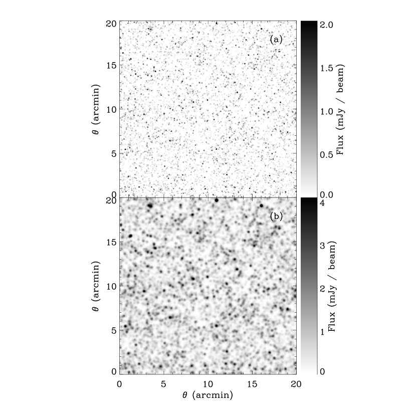
Figure 1: Simulated maps of the millimeter sky. These are based on the L50/144 simulation, using our fiducial SED of $T=35\,\mbox{K}$, $\beta=1.0$, and are generated by the randomization procedure discussed in the text. (a) This map is “measured” at a wavelength of 1.2 mm with a resolution of 6 arcsec, appropriate to the Large Millimeter Telescope (LMT) currently under construction. The map is normalized such that a pixel centered on a source with a given flux corresponds to the gray scale level in the color bar. (b) This map uses a wavelength of 850 µm and assumes a resolution of 15 arcsec appropriate to SCUBA on JCMT. Although SCUBA maps are usually quite noisy, no noise is included in this or the previous map.

4.1 Distribution in flux

Using the catalogs of fluxes from each galaxy in the simulation, we calculate the counts on the sky as a function of flux at 850 µm. The counts that result from using only the L50/144 simulation, and single-temperature models, are shown in Figure 2. This plot demonstrates the large effect that the uncertainty in the SED can have on the predicted counts. The emission models used span most of the range usually considered for the sub-mm sources. Raising either $T$ or $\beta$ depresses the calculated fluxes by reducing the 850 µm luminosity for a given bolometric luminosity. Also, $T$ and $\beta$ are nearly degenerate in their effect on the counts, as one can see, for example, by comparing the curves for $T=40\,\mbox{K}$, $\beta=1.0$ and $T=35\,\mbox{K}$, $\beta=1.3$. As discussed above, the short-wavelength slope $\alpha$ could shift the curves leftward by tens of percent. The uncertainty in $f_{SF}$ could also shift the curves horizontally by as much as a factor of two (in either direction).

Some of the results from SCUBA surveys of galaxies are presented on the plot, with their source marked in the legend. The many different surveys and the large scatter they exhibit deserve some explanation. The solid symbols show the results of blank-field surveys (Barger, Cowie & Sanders 1999; Eales et al. 2000; Borys et al. 2001; Dunlop 2001). The lensing cluster surveys (Blain, Ivison, Kneib & Smail 1999; Chapman et al. 2000a) have two advantages stemming from the magnifying effect of the cluster: they can go deeper in flux, and source confusion is reduced. However, the necessary correction for the cluster lensing amplification introduces some risk of systematic error.

Since this is a cumulative plot, the data points are correlated in any given survey. Also, the error bars generally account for Poisson errors only and thus may be underestimated.

The raw counts are strongly affected by observational biases, because of the poor spatial resolution and S/N currently available. Eales et al. (2000) argue that the combined effect of noise and confusion amplifies the measured source fluxes by about a factor of 1.4 on average in their survey, independent of flux. We have thus shown in gray their survey, and the similar survey of Barger, Cowie & Sanders (1999), corrected down by this factor. However, this argument is controversial, with other workers disagreeing on the constancy (Blain, 2000) or even the sign (Hughes & Gaztañaga, 2000) of the effect. It is also unclear whether the cluster surveys, or the higher flux limit, blank-field surveys (Borys et al., 2001; Dunlop, 2001), are affected by confusion; if not, the disagreement in the measured counts is even greater at the high-flux end.

The sub-mm observations are still clearly in their early stages, and the present results have a large scatter that is not all due to random statistical errors. If we take our results with $T\approx 35\,\mbox{K}$ and $\beta=1.3$, roughly the mean parameters found in the local SCUBA survey (Dunne et al., 2000), we appear to have a reasonable fit to the lower envelope of the observations defined in part by the confusion-corrected points. This model would produce an integrated 850 µm background of $12.9\pm 4.7\,\mbox{mJy}\,\mbox{arcmin}^{-2}$, which agrees with the background measurement from FIRAS, $(12.2\pm 4.7)\,\mbox{mJy}\,\mbox{arcmin}^{-2}$ (Fixsen et al., 1998). The background measurements from DIRBE (Hauser et al., 1998) exceed those from FIRAS by about 40% at shorter wavelengths, although the two measurements are formally consistent, so the true background may be slightly higher. This SED is at the “cold” end of the parameters usually considered for sub-mm sources, an issue we return to in § 4.3.

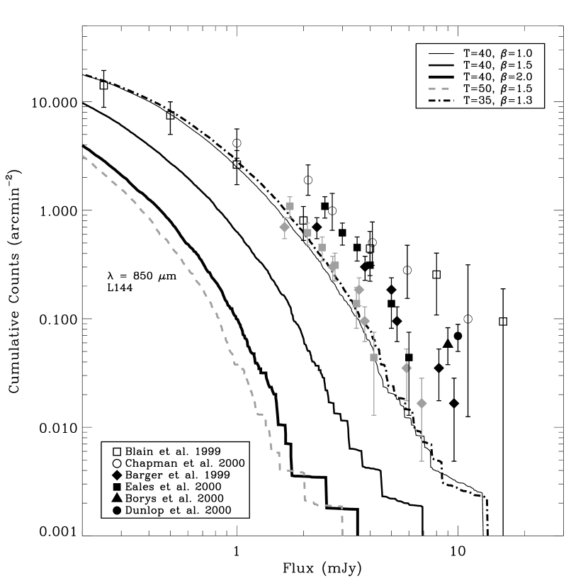
Figure 2: Cumulative counts as a function of flux at 850 µm, for some single-temperature models. Only the galaxies from the L50/144 simulation are included here. The SED parameters of the models are marked in the legend. The various observational points are discussed in detail in the text; open points come from lensed cluster fields, filled points come from blank-field surveys, and grey points incorporate an approximate (and somewhat controversial) correction for observational biases. For the models listed in descending order in the figure legend, the integrated backgrounds at 850 µm are 12.2, 6.2, 3.0, 2.7, and $12.9\,\mbox{mJy}\,\mbox{arcmin}^{-2}$.

While this model is in agreement with the lowest of the observational points, it is hard to escape the impression in Figure 2 that the true counts are somewhat higher. (Whether this is so depends largely on the validity of the confusion correction introduced by Eales et al. 2000.) It is interesting to see what kinds of models are required for the simulations to match the raw blank-field or the cluster survey counts instead. In Figure 3 we show three attempts to accomplish this match. The first model simply adopts yet smaller SED parameters of $T=35\,\mbox{K}$, $\beta=1.0$. The second model uses a larger $f_{SF}=8\times 10^{9}L_{\sun}\,M_{\sun}^{-1}\,\mbox{yr}$, with $T=35\,\mbox{K}$ and $\beta=1.3$, and produces similar results to the first. In both cases the simulated counts may be steeper than the observations.

The third and fourth altered models allow for random scatter in the galaxy SEDs, as discussed in § 3. In a real galaxy the factors determining dust emission are surely not “random”, but this model reflects our ignorance of what causes the variation in the FIR SEDs of local galaxies. We find that the counts become significantly shallower in this case, improving the agreement with the blank field surveys. A mean temperature of $T=35\,\mbox{K}$ gives a good fit to the uncorrected counts, while a temperature of $T=38\,\mbox{K}$ provides a better fit to the confusion-corrected points.

Because of its physical plausibility and its reasonable success in matching the uncorrected blank-field counts, we choose the $T=35\,\mbox{K}$, $\beta=1.0$ model as our fiducial model for the rest of the paper (e.g., for Figures 1 and 7–9). However, to zeroth order, choosing a different $T$ and $\beta$ combination affects the fluxes from all galaxies in the same way, although there are first order differences depending on redshift. Hence, any such combination that fits the uncorrected counts will contain essentially the same objects at any given flux or counts threshold, and thus imply almost the same physical properties. Also, if one accepts the shift in the fluxes suggested by Eales et al. (2000), the preferred SED parameters change as discussed above; but the implied physical properties for a given flux-limited sample should be almost the same if one simply lowers the flux thresholds by a factor of 1.4.

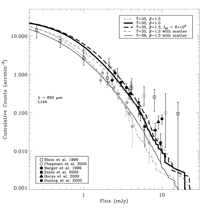
Figure 3: Similar to Figure 2, but the predicted counts use modified emission models that raise the counts at high fluxes as explained in the text. For the models listed in descending order in the figure legend, the integrated backgrounds at 850 µm are 12.9, 18.7, 20.7, 15.2, and $11.3\,\mbox{mJy}\,\mbox{arcmin}^{-2}$.

So far, the calculated counts use only the L50/144 simulation. However, the typical star formation rate at a given baryonic mass is higher at high redshift (when gas accretion rates are higher), so the minimum star formation rate that is resolved in any given simulation rises towards higher $z$. With our preferred flux models, this resolution threshold begins to affect the counts at the 2 mJy level by $z\sim 3$ in the L50/144 simulation. To examine the effect of resolution, we use the artificial high-resolution sample discussed in §2. Since this sample is generated from an analytic fit rather than an actual simulation, it should be viewed as merely illustrative of the effect of higher numerical resolution. However, its properties are well constrained by the behavior in the low and high resolution simulations.

Figure 4 illustrates the effect of this extended high-resolution sample on the simulated counts. For each model, we show the results obtained both with the extended sample and with the L50/144 simulation alone. Extending the sample makes a significant difference below 1 mJy. The models that best agree with the observed counts above 1 mJy no longer agree below that level, and their cumulative surface brightness now exceeds the FIRAS background. Since the background values obtained using only the L50/144 simulation are acceptable, a cutoff in the opacity at $\sim\!60\,M_{\sun}\,\mbox{yr}^{-1}$ could produce agreement, but this cutoff value is likely too high.

The predicted excess of faint sources seen in Figure 4 may be a genuine problem for our model. However, at low luminosities and $z<3$, our analytic fit to the SFR function is constrained mostly by the small L11/64 simulation; hence uncertainty in the fit could be the cause of the discrepancy. The background excess could also be influenced by our simplistic extinction model. In this paper we are mainly interested in the objects above 1–2 mJy, so we postpone a detailed examination of this issue to a future paper (Fardal et al., 2001).

The counts in the L50/144 simulation may be incomplete at the bright end as well, due to the finite volume and consequent exclusion of long-wavelength modes. This probably occurs at a counts level of $\sim\!0.01\arcmin^{-2}$, or a flux level of $\sim\!10\,\mbox{mJy}$ with our fiducial model, though it is difficult to confirm this without running a simulation in a yet larger volume.

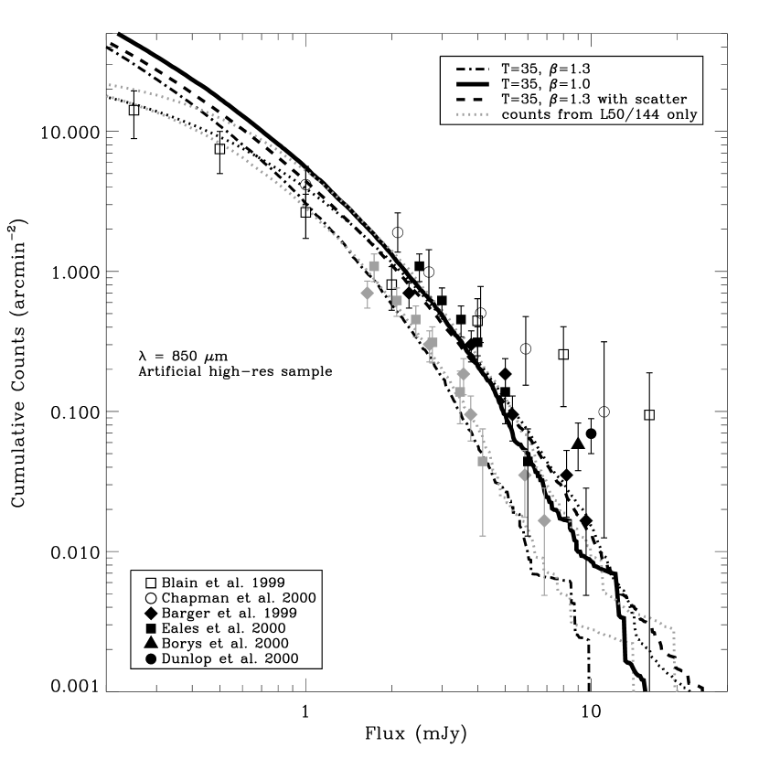
Figure 4: Similar to Figure 3, but using results of the artificial high-resolution sample. Two of the models from the previous figure are omitted here for clarity. The dotted lines show the results of the L50/144 simulation for comparison. They use the same set of emission models, and match onto the corresponding high-resolution curves at about 1 mJy. For the models listed in descending order in the figure legend, the integrated backgrounds at 850 µm from the high-resolution sample are 27.4, 37.3, and $31.3\,\mbox{mJy}\,\mbox{arcmin}^{-2}$.

With the best-fitting emission models here, the star formation rates implied for the SCUBA galaxies are large, though smaller than some estimates. For example, at $z=2.5$, a galaxy with ${\it SFR}=100\,M_{\sun}\,\mbox{yr}^{-1}$ has a flux of $1.2\,\mbox{mJy}$ at 850 µm, assuming our fiducial model of $T=35\,\mbox{K}$ and $\beta=1.0$. For comparison, the flux would be only $0.16\,\mbox{mJy}$ using $T=40\,\mbox{K}$, $\beta=1.5$, $\alpha=-2.2$, and $f_{SF}=2.2\times 10^{9}L_{\sun}\,M_{\sun}^{-1}\,\mbox{yr}$ as in Blain et al. (1999b).

4.2 Distribution in redshift

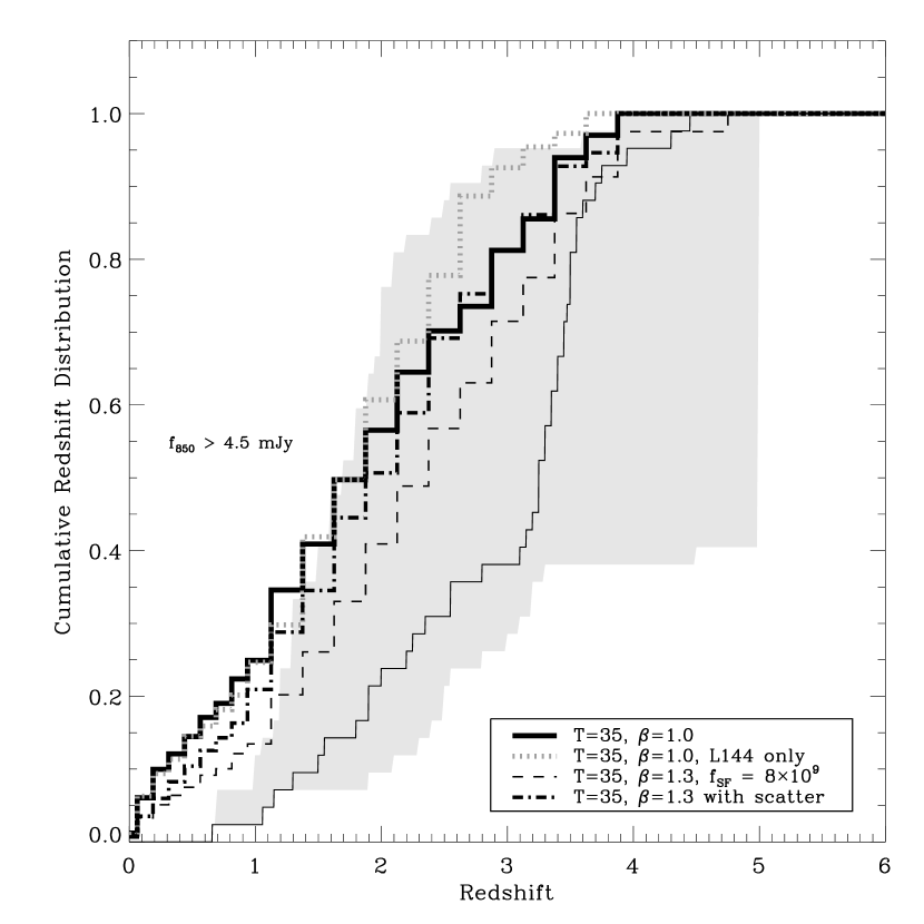
Figure 5: The cumulative redshift distribution of the 850 µm sources. The gray shaded region and the light solid curve bisecting it represent the observational limits and mean estimates, respectively, from the combined results of Barger, Cowie & Richards (2000); Smail et al. (2000) and Eales et al. (2000). The curves marked in the legend are based on our simulation, using various emission models and assuming a sample threshold of $4.5\,\mbox{mJy}$. The stair-step appearance in the simulation lines results from the use of discrete outputs. The steps in the observational results are from individual sources.

The cumulative redshift distribution of the sources is shown in Figure 5. Here we assume a flux threshold $f(850\,\micron)>4.5\,\mbox{mJy}$, comparable to the observational samples discussed below. The distribution is actually bimodal, as shown by the subtle minimum of the slope at $z\sim 0.5$. The broad high-redshift portion extends to $z\approx 4$. Using our fiducial SED model and the artificial high-resolution sample, the median redshift for the 4.5 mJy sample is 2.0; the mean and standard deviation are 2.0 and 1.3. Using only the L50/144 simulation lowers the redshifts, with a median of 1.8, mean of 1.8, and standard deviation of 0.9; the shifts are small because of the high sample threshold. Using a higher $\beta$ and $f_{SF}$ as indicated in the legend increases the median redshift to 2.4, with a mean of 2.3 and standard deviation of 1.2. If the Eales et al. (2000) confusion correction is applied to all fluxes in these redshift surveys, an appropriate model as discussed above is $T=35\,\mbox{K}$, $\beta=1.3$, and our standard $f_{SF}$; but in this case one should use a sample threshold of $\sim\!3.0\,\mbox{mJy}$. Since lowering the flux threshold and raising the fluxes from all the objects are equivalent changes, the resulting distribution is nearly identical to the curve with the non-standard $f_{SF}$.

The predicted redshift distribution is not strongly affected by our choice of SED among the alternatives we prefer above. The main impact is to change the balance of the low-$z$ and high-$z$ components. The bimodal distribution arises in our simulation for the following reason. At high $z$, the flux from a source of a given luminosity is nearly constant, but the flux rapidly increases as $z^{-2}$ for $z\ll 1$. The mean luminosity of our sources brightens as a power-law in $(1+z)$ at low $z$, so the characteristic flux reaches a minimum at $z\sim 0.5$. The low-$z$ component is boosted by the low values of $\beta$ in our preferred models. Changing the threshold flux also changes the balance of the low-$z$ and high-$z$ components. Above 10 mJy we find that about half of the sources are at $z<0.5$ for our fiducial model. However, at this flux level the counts in our simulations are very incomplete at high $z$, due to finite-volume effects. For a threshold of 2 mJy, we find instead a higher median redshift of 2.3 for our fiducial model.

Observational constraints on the redshift distribution of the sub-mm population are still fairly weak. Few sources have spectroscopic redshift measurements, so most of the redshifts are estimates based on the radio-FIR correlation. The derived redshift is dependent on the assumed SED, and is roughly proportional to $T$. In many cases the radio emission is undetected, giving only a lower limit to the redshift. The redshift estimates and limits from Smail et al. (2000), Barger, Cowie & Richards (2000), and Eales et al. (2000) all assume a set of SEDs to obtain the allowed redshift ranges. We have combined them here without regard to the slightly different SEDs employed.

Assuming a maximum redshift of $z_{\it max}=5$ for all sources, we have placed the observed sources at their lower redshift limit, their upper redshift limit, or at the middle of the range (the limits are taken from the observational papers and are $\sim\!2\sigma$). The extreme assumptions give the shaded region in Figure 5, while the middle assumption gives the solid line bisecting this region. Most of the difference between these curves is systematic error due to the uncertainty in the SED. With the lower values of $T$ and $\beta$ that we prefer above, the redshift distribution would be close to the left hand boundary. The mean of the estimated redshifts (i.e., the middle curve, which assumes higher SED parameters than preferred here) is 2.9, and the median is 3.3. The dispersion in the estimated redshifts of the sources is 0.91. Of course, some of this dispersion could be due to scatter in the SED or the radio emission properties, or to observational error.

Our redshift distribution is in fairly good agreement with these results, with a similar mean (once the effect of the SED is accounted for) and width. We do appear to have an excess of predicted sources at $z<1$. This excess could be related to the large amount of low redshift star formation in our simulations. We are currently investigating this issue with a larger set of simulations (Fardal et al., 2001). The brightest observed sources could include sources that are primarily AGN, which we do not include in our modeling here; their inclusion would probably boost the predicted median redshift.

4.3 The SED of the sub-mm sources

The SED parameters of our preferred models are consistent with low-redshift observations of FIR-bright galaxies (Dunne et al., 2000). Somewhat higher temperatures have generally been preferred for SCUBA sources in the literature, however, which raises the question of whether our temperatures are too low to be plausible. Smail, Ivison & Blain (1997) preferred a temperature of $60\,\mbox{K}$ and described $T=40\,\mbox{K}$ as “very cold”. Other choices have included $T=47\,\mbox{K}$, $\beta=1.0$ (Barger et al., 1998); $T=50\,\mbox{K}$, $\beta=1.5$ (Hughes et al., 1998); and $T=40\,\mbox{K}$, $\beta=1.5$ (Blain et al., 1999a). Changing $f_{SF}$ by a reasonable amount would bring our best-fit temperatures into this range, as shown above.

As noted by Eales et al. (2000), the argument that the majority of SCUBA sources are ultraluminous infrared galaxies (ULIRGs) is somewhat circular. If the temperatures are assumed to be 40–60 K, typical of local ULIRGs, rather than 20 K, typical of local normal spirals, one finds that the sources have the bolometric luminosity of a ULIRG, but lower assumed temperatures would imply lower luminosities. Escaping the circularity requires redshifts and multiwavelength observations of sub-mm sources without evidence of AGN activity. There are only a few such sources at present (see discussion in Blain 1999). These do seem to have temperatures of roughly 40–50 K, though the limits are not stringent. In principle, an understanding of the dust mass implied by a given SED combined with an upper limit on the metals in a galaxy’s ISM can give lower limits on the temperature. The temperatures assumed in our best-fit models do not appear to violate these limits.

Some direct evidence regarding the SEDs of SCUBA sources comes from the 450 µm measurements of Eales et al. (2000), who derived a $3\sigma$ upper limit of $\langle S_{450}\rangle/\langle S_{850}\rangle<2.4$ for their 850 µm-selected SCUBA sample. Eales et al. argue that this limit implies surprisingly low dust temperatures ($T\lesssim 25$, if $\beta=2.0$) for the sub-mm sources. However, we disagree with this inference. First, if we accept their argument that their 850 µm fluxes are biased high by a factor 1.4 from observational confusion, this limit increases to 3.4. Second, Eales et al. (2000) assume a fixed redshift to argue that the temperatures are low. However, these redshifts are ultimately themselves based on an assumed SED, because they are almost entirely based on the radio-sub-mm flux ratio. As discussed by Blain (1999), this ratio depends essentially on the combination $T/(1+z)$. The 450/850 µm flux ratio depends on the same combination of parameters. Hence assuming cool dust temperatures alters the implied redshifts, and there is little net effect on the 450/850 µm ratio; the two parameters are degenerate with respect to these two flux ratios.

However, the effects of $\beta$ and $(1+z)/T$ on the 450/850 µm and radio/sub-mm ratios are not entirely degenerate; $\beta$ has a stronger influence on the former ratio than the latter. Hence the low 450 µm fluxes seem to suggest low values of $\beta$. Let us make a simple calculation, representing the entire sub-mm population by a single “typical” source. We calibrate the radio luminosity using the results for low-redshift IRAS sources of Yun, Reddy, & Condon (2001). Including their conversion factor of 1.5 between IRAS luminosity and total dust luminosity $L_{\it bol}^{\it{}(dust)}$, the implied FIR-radio correlation is $S_{1.4GHz}=3.1\times 10^{18}\,\mbox{erg}\,\mbox{s}^{-1}\,\mbox{Hz}^{-1}(L_{\it bol}^{\it{}(dust)}/L_{\sun})$. We also assume a radio continuum slope of $-0.8$. We require that the 850 µm / 1.4 GHz ratio be 100, typical of the sub-mm source population, and the 450/850 µm ratio be $<3.4$. Then we find the limits $\beta\lesssim 1.0$ and $(1+z)/(T/40K)\lesssim 2.8$. Admittedly, this calculation is crude and the input parameters are fairly uncertain. However, it does seem to support the low values of $\beta$ used in our preferred SEDs.

Unfortunately, further multiwavelength observations of the FIR continuum alone will be just as inadequate in disentangling the temperature and redshift. The key to determining the source SEDs is to obtain the source redshifts by some other means: from optical spectroscopy or photometry, mid-IR spectral features, or molecular lines. At this point, we know very little about the correct choice of SED, which is so important when comparing the simulations to observations. All we can say is that the observations may marginally favor the lower $\beta$ values that we have suggested, and do not contradict the lower values of $T$.

To summarize our results in this section, there is a galaxy population in our simulations that corresponds to the observed sub-mm sources, but only if the dust temperatures are sufficiently low or the stellar energy output is sufficiently high. To zeroth order the agreement is acceptable, although the counts may be somewhat too steep and there may be too many low-redshift objects compared to current observations. We now go on to describe the physical properties of these galaxies.

5 PHYSICAL PROPERTIES OF SUB-MM GALAXIES

In general, our sub-mm sources are quite massive galaxies, as shown in Figure 6. In a flux-limited sample with $S_{850}>1\,\mbox{mJy}$, the mass in cold gas and stars has a median of $M_{b}\gtrsim 1.3\times 10^{11}\,M_{\sun}$ at $z=2.5$ (assuming $T=35\,\mbox{K}$ and $\beta=1.0$), and the median mass increases with increasing flux threshold ($3.8\times 10^{11}\,M_{\sun}$ for 3 mJy and $4.4\times 10^{11}\,M_{\sun}$ for 6 mJy). The distribution is quite broad, however. If we choose instead an SED with $T=35\,\mbox{K}$ and $\beta=1.3$, the star formation rate at a given flux increases by a factor of 1.4; since the star formation rate is roughly proportional to mass, the masses at a given flux threshold also increase approximately by this factor. The stellar mass distribution (not shown here) is yet broader, with a median stellar mass of $6.6\times 10^{10}\,M_{\sun}$ at 1 mJy, again increasing with flux.

We can define a timescale for star formation in these galaxies by taking this median mass over the median star formation rate of $116\,M_{\sun}\,\mbox{yr}^{-1}$, giving a typical timescale of $0.60\,\mbox{Gyr}$. For reference, the cosmic time is $2.4\,\mbox{Gyr}$ at $z=2.5$. Thus the high star formation rates of our simulated galaxies are not just due to extremely short bursts. This conclusion is also implied by the correlation at high redshift between star formation rate and mass in our simulations, particularly for the high-mass objects (Weinberg, Hernquist, & Katz, 2000). If discrete bursts were the dominant cause of the high luminosities, they would tend to randomize the mass-luminosity correlation. We note that if the emission model contains random scatter as discussed above, the distributions of the flux-limited samples in Figure 6 become broader, but the general trends remain.

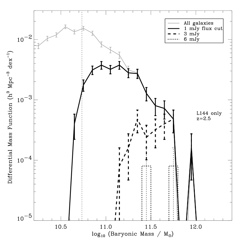
Figure 6: The distribution of baryonic mass in cold gas ($T<3\times 10^{4}\,\mbox{K}$) and stars for the simulated galaxies. The plot uses the L50/144 simulation and assumes the fiducial SED model ($T=35\,\mbox{K}$, $\beta=1.0$). Sub-samples selected by sub-mm flux are shown by the curves marked in the legend. Error bars assume Poisson statistics.

Another way to characterize the size of our sub-mm galaxies is to find their circular velocities $V_{c}$. However, if the galaxies live in groups or clusters, there could be an important distinction between the circular velocity of the galaxy itself and that of the largest virialized structure containing it. To tackle this question, we first use the program FOF to group dark matter particles into halos by the friends-of-friends algorithm, using a linking length appropriate to the mean interparticle spacing at the edge of a virialized halo (Kitayama & Suto, 1996). We center a sphere on each sub-mm galaxy and measure $V_{c}$ at a radius of 10 physical $h^{-1}\,\mbox{kpc}$, the smallest reasonable radius given our spatial resolution of $2h^{-1}\,\mbox{kpc}$ at this redshift. We also center the sphere on the most bound particle in the FOF halo to which the sub-mm galaxy belongs, and measure $V_{c}$ at the radius where the density matches the virial density.

The circular velocities defined at $10h^{-1}\,\mbox{kpc}$ and at the halo virial radius are not greatly different, at least at $z=2.5$. The median $V_{c}$ of the 1, 3, and 6 mJy samples are 328, 500, and $569\,\mbox{km}\,\mbox{s}^{-1}$ for the galaxies themselves at $10h^{-1}\,\mbox{kpc}$. They are 282, 403, and $495\,\mbox{km}\,\mbox{s}^{-1}$ for their surrounding virialized halos at the virial radius. It is not surprising that the galaxy circular velocities somewhat exceed those of their surrounding dark matter halos. Each sub-mm galaxy tends to be the dominant baryonic object in its neighborhood, with a mass large enough to increase the circular velocity at $10h^{-1}\,\mbox{kpc}$. At these redshifts, large virialized structures with velocity dispersions characteristic of clusters (and higher than those of their central galaxies) have yet to form. The high circular velocities, substantially higher than those of $L_{*}$ galaxies today, confirm that the sub-mm galaxies in this simulation are massive objects residing in massive dark matter halos.

We have computed the time evolution of the L50/144 simulation up to the present day, so we can directly measure the lifetimes of the sub-mm sources. To do this, we define various 850 µm flux-limited samples of simulated galaxies, assuming $T=35\,\mbox{K}$ and $\beta=1.0$. We then construct a merger tree of all of these galaxies down to $z=0$, using the same methods as in Murali et al. (2001). Restricting our study to the redshift interval $1<z<4$, which includes most of the SCUBA sources (c.f. Figure 5), we find the distribution of lifetimes for sub-mm sources as shown in Figure 7. Our time resolution is limited by the spacing of our discrete simulation outputs, which varies from $0.1\,\mbox{Gyr}$ at $z=4$ to $0.7\,\mbox{Gyr}$ at $z=1$. If a source does not repeat (i.e., appear in more than one output), we assume that it lasts for less than 0.1 Gyr. With higher time resolution, therefore, the time distribution curves would be higher at lifespans $<0.7$ Gyr, but the fraction of non-repeating sources is small, so this should not be a large effect. Of course, we are unable to tell whether the emission from a given galaxy turns off briefly between outputs; but if our sub-mm sources were constantly flickering on and off, this would only reduce the apparent lifetimes. The mean age of a 3 mJy source is $\sim 500$ Myr, although a significant fraction of our sources remain sub-mm sources for more than 1 Gyr. The contribution to the background is even more heavily weighted towards the long-duration sources than is apparent in Figure 7, as they tend to have larger luminosities. For example, considering the sources in the 1 mJy sample over the interval $1<z<4$, the sources that repeat at least one time have an average flux of 1.9 mJy, compared to 1.3 mJy for those that do not. Inspecting some of the nonrepeating sources, we find that they too are sources with slowly varying star formation rates, which are just cresting over the sample threshold. Similar conclusions apply at higher flux thresholds as well.

Figure 7: Cumulative distribution of the lifespan of a sub-mm source, over redshifts $1<z<4$ in the L50/144 simulation. The distribution is effectively weighted by the time a galaxy stays a sub-mm source, since this is the way it would appear in an observational sample. The curves show results for different flux-limited samples. The spacing of our outputs increases from 0.1 Gyr at $z=4$ to 0.7 Gyr at $z=1$, and we assign a lifespan $<0.1$ Gyr to any source that does not appear in consecutive outputs. With higher time resolution, the true distribution would thus be higher than the plotted curves below 0.7 Gyr.

We can also follow the star formation in individual galaxies over cosmic time. While there is some rapid variation in the star formation rates of these galaxies, the amount of such “noise” is typically less than a factor of 2, and the variation in star formation rate is typically dominated by slow evolution scales of about a Gyr. (c.f. Weinberg, Hernquist, & Katz 2000). Our overall conclusion is that our simulated sub-mm sources are forming large numbers of stars in a fairly steady way at high redshifts.

Because they are so massive, the sub-mm galaxies in our simulation are strongly clustered. Over the redshift range $1<z<4$, their spatial correlation length is about 4–$5h^{-1}\,\mbox{Mpc}$, with a correlation power-law exponent $\gamma\approx 2.0$. For $1<z<3$, the correlation amplitude is enhanced relative to the average galaxy resolved in our simulation by a factor of $\sim 1.7$. However, this strong clustering will be difficult to detect observationally, because these sources are spread out over a wide range of redshifts. Direct measurement of the redshift-space correlation function requires an accurate redshift survey of the sub-mm sources, something that will not be achieved for some time.

We can predict the angular clustering of sub-mm sources using the simulated maps described at the beginning of §4. The angular correlation function of sources with fluxes above 1 mJy is approximated by $w(\theta)\approx 0.02(\theta/\,\mbox{arcmin})^{-0.9}$ over a range 0.04 to 10  arcmin. This angular clustering is about a factor 3 lower than that of the Lyman break galaxies (Giavalisco et al., 1998), which is accurately reproduced in our simulations (Katz, Hernquist, & Weinberg, 1999). The reason for the weaker angular clustering of the sub-mm sources is simply that the stronger three-dimensional clustering is offset by a larger redshift depth. To quantify the angular clustering of the 1 mJy sources to 10%, a survey area of about 5 square degrees will be required. This is a much larger survey than available at present, but it could be easily achieved with the LMT.

The merger trees for our sub-mm sample allow us to follow the sub-mm sources in the L50/144 simulation to the present day. We define a sub-mm descendant here as a galaxy whose merger tree contains a sub-mm source in the redshift range $1<z<4$. Of course, these galaxies often contain other material as well. In some cases the particles from a sub-mm source form only a small part of the mass of a central cD-like cluster galaxy.

Naturally, we find that the sub-mm descendants are quite massive, since the sub-mm sources were already quite massive. We can examine the stellar population of these descendants as well. The simulation records each star formation event as it takes place, so we can find the star formation history of any given galaxy. Figure 8 plots the median star formation time for each galaxy in the simulation, versus the total baryonic mass of the galaxy. The sub-mm descendants are shown as the more prominent points. While the sub-mm descendants are usually massive, there are some that are among the less massive galaxies. However, they are almost universally among the oldest galaxies in the simulation, in terms of their stellar population. The vertical lines show the time range in which the middle 80% of the stars formed, for a few randomly chosen galaxies. One can see that the star formation is quite extended, agreeing with our depiction of steady star formation. In the real universe, the oldest galaxies are giant cluster ellipticals, which seem to have formed most of their stars before $z\gtrsim 2$ (Bower, Lucey & Ellis, 1992; Stanford, Eisenhardt & Dickinson, 1995). Few galaxies in our simulation have a median star formation redshift as high as $z=2$, but we only have two galaxy clusters in our simulation and they are only the size of the Virgo cluster. Spheroidal populations, i.e. ellipticals and bulges, may have a smaller median age (Zepf, 1997; Fontana et al., 1999). Qualitatively, however, the large ages shown in the figure suggest an identification with elliptical galaxies.

Figure 8: Median formation time of stars in the simulated galaxies versus their baryonic mass in cold gas and stars. This plot uses only the L50/144 simulation. More recent formation is at the top of the figure. For randomly selected galaxies, we have also shown the range where the middle 80% of the stars were formed. Filled squares and solid lines show descendants of the galaxies that were brighter than 1 mJy at 850 µm at some redshift in the range $1<z<4$, using the fiducial SED model. Open circles and dotted lines show the remaining galaxies.

The descendants of the sub-mm sources are also highly clustered. One way to measure this is by the circular velocities of their surrounding environments. We measure the circular velocities of the virialized dark matter halos in the same way as discussed above. Then, we define “cluster” and “group” halos by the requirements $V_{c}>700\,\mbox{km}\,\mbox{s}^{-1}$ and $350\,\mbox{km}\,\mbox{s}^{-1}<V_{c}<700\,\mbox{km}\,\mbox{s}^{-1}$ respectively. With these definitions, 79% of all galaxies in our L50/144 simulation reside in the field, 18% in groups, and 3.2% in clusters at $z=0$. In contrast, 57% of our sub-mm source descendants reside in the field, 35% in groups, and 6.6% in clusters. Another way to show the strong clustering is to examine the fraction of galaxies that are sub-mm descendants as a function of local galaxy number density. We find a trend quite similar to the well-known density-morphology relation (e.g., Postman & Geller 1984), but even more extreme, with almost no descendants below number densities of $0.1h^{3}\,\mbox{Mpc}^{-3}$.

It has been suggested that the sub-mm sources are massive ellipticals in the process of formation. One argument for this is that elliptical galaxies have old stellar populations, as shown (at least in clusters) by their tight color-magnitude relation (Bower, Lucey & Ellis, 1992) and the passive evolution of their colors (Stanford, Eisenhardt & Dickinson, 1995). This suggests, although it does not prove, that the galaxies themselves were formed at high redshift. Another argument is the common hypothesis that ellipticals were formed in mergers, coupled with the observation that ULIRGs at low redshift are typically mergers in progress. If the high-redshift sub-mm sources are similar to the low-redshift ULIRGs, this supports the notion that they mark the birth of ellipticals.

In the L50/144 simulation, our spatial resolution is too low to resolve the morphology of our galaxies and distinguish spirals from ellipticals. However, several features of the sub-mm source descendants—high mass, old stellar populations, and strong clustering—do indeed suggest that they correspond to massive ellipticals in the process of formation. Still, we emphasize that in our simulations the sources usually do not owe their high luminosities to very short bursts. Our sub-mm galaxies instead form in a more gradual manner over periods of $\sim\!0.1$–$1\,\mbox{Gyr}$.

6 DISCUSSION

The results presented in this paper amount to a physically motivated model for the population of sub-mm galaxies detected in the SCUBA surveys. The underlying basis of this model is the $\Lambda$-dominated cold dark matter cosmological scenario, coupled to our numerical methods for following gravitational evolution, gas dynamics and cooling, and star formation. The essential features of the star formation algorithm are a gas consumption timescale that decreases steadily with increasing gas density, feedback effects that are relatively modest, at least in the massive galaxies that correspond to sub-mm sources, and an IMF similar to that inferred in the solar neighborhood (Miller & Scalo, 1979). Given our numerical simulation of the population of star-forming galaxies, the main uncertainty in our predictions comes from the choice of FIR spectral energy distribution. Matching the observed sub-mm counts requires values of the SED parameters $T$ and $\beta$ that are fairly close to those inferred for IR-luminous galaxies in the local universe by Dunne et al. (2000), but these values are lower than those used in most models of the SCUBA population. Our default model has $T=35\,\mbox{K}$, $\beta=1.0$, but the values of $T$ and $\beta$ have nearly degenerate effects, scatter in the SEDs would yield similar counts for higher $T$ and/or $\beta$ values, and the overall factor for converting star formation rate to bolometric luminosity is itself uncertain at the factor of two level.

The essential features of this model are that the sub-mm population is broadly distributed in redshift, with a median $z\approx 2-2.5$, and consists mainly of massive galaxies forming stars fairly steadily over timescales $\sim 10^{8}-10^{9}$ years at rates of $\sim 100\,M_{\sun}\,\mbox{yr}^{-1}$. The descendants of these sub-mm sources are even more massive galaxies, with old stellar populations, found primarily in dense environments. At a qualitative level, these properties support the identification of sub-mm sources with the progenitors of luminous early-type galaxies.

The steady star formation and correspondingly moderate star formation rates are what distinguish this model of the sub-mm population from some of the alternative pictures proposed in the literature (discussed further below). While the typical formation timescales are still a factor of a few shorter than the cosmic time at the same redshift, they are much larger than, e.g., the timescale of $\sim 2\times 10^{6}$ yrs suggested for FIR emission by Thronson & Telesco (1986). Typical star formation rates of $\sim 100\,M_{\sun}\,\mbox{yr}^{-1}$ require, in turn, relatively low values of $T$ and/or $\beta$ to yield sufficient flux at sub-mm wavelengths.

The principal successes of this model are its ability to reproduce the bright ($>1\,\mbox{mJy}$) sub-mm counts and its consistency with existing constraints on the source redshift distribution (Figure 5). Unfortunately, the first cannot be counted as a major success because of the large observational uncertainties and the substantial freedom to change the predicted fluxes by reasonable alternative SED choices. We did not make any adjustments to match the redshift distribution, so success there is reassuring, though the model does predict a potentially significant excess of low-redshift sources. The model also has difficulty matching source counts above $10\,\mbox{mJy}$, though these could be affected observationally by contributions from AGN and by lack of large-scale power in our finite simulation volume.

Another, potentially more serious failing of this model is its prediction, once we correct for numerical resolution effects, of too many faint sources and an excessively high 850 µm background (see Figure 4). We will save detailed discussion of this issue for a future paper (Fardal et al., 2001), but a few comments are in order here. Part of this problem may simply be due to the small volume of the L11/64 simulation we used to constrain the properties of smaller objects at low redshifts. Overproduction of faint counts and the sub-mm background, and the possible excess of low redshift sources mentioned above, could be connected to other possible shortcomings of the simulated galaxy population that we have noted elsewhere (e.g., Katz, Weinberg, & Hernquist 1996; Weinberg et al. 1999; Aguirre et al. 2001): an excess of low redshift star formation and an overly high fraction of baryons converted into stars. Balogh et al. (2001) have argued that the latter problem is generic to simulations of this sort and can only be solved by appealing to much more vigorous feedback effects from star formation (see Cole et al. 2000 for discussion of similar problems in semi-analytic models). While we agree that feedback could be a solution, there are many other possibilities, including: observational errors in the stellar density (see, e.g., the discussions of luminosity function discrepancies by Cole et al. 2001, Blanton et al. 2001, and Wright 2001); numerical errors causing the simulations to systematically overestimate gas cooling; changes to the cosmological model such as reduced initial power on galactic scales or lower baryon density; or an initial mass function (at least in some galaxies) that contains a large mass fraction of brown dwarfs or differs systematically from the solar neighborhood IMF in some other way. We note also that if feedback alone is to reconcile the simulations with the sub-mm source counts at $\sim\!1\,\mbox{mJy}$, then it must be effective in galaxies with baryon masses $\sim\!5\times 10^{10}M_{\odot}$ (see Figure 6), not just in low mass systems.

An obvious risk is that any change to our model that reduces the faint source counts and sub-mm background will also spoil the agreement with bright source counts. A luminosity-dependent SED is possible, and perhaps even probable. A luminosity-dependent IMF could similarly improve the agreement. Both, however, represent unattractively ad hoc solutions at present. Another generic way to make the predicted source counts flatter would be to make star formation episodic, so that more of the bright sources correspond to more common, low mass objects caught during a burst of star formation. In particular, it is possible that our simulations underestimate the importance of merger-induced starbursts because of their limited resolution. In their simulations of galaxy mergers, Hernquist & Mihos (1995) and Mihos & Hernquist (1996) found bursts of star formation enhanced by a factor 10–100 over the star formation in isolated galaxies. The resolution in our cosmological simulation may simply be too poor to obtain such large bursts, or the large particle-induced noise may prevent the buildup of large gas reservoirs. Whereas each galaxy in the Mihos & Hernquist simulations was represented by about $3\times 10^{4}$ gas particles, our galaxies often contain only a few hundred, and they do not resolve galactic disks. Observationally, we know that low-redshift mergers produce enormous bursts of star formation (Sanders & Mirabel, 1996).

On the other hand, there are reasons to suspect that bursts and mergers do not play a dominant role in the global history of star formation, even if they are important in some objects. From this same L50/144 simulation, Murali et al. (2001) conclude that smooth accretion dominates over merging by at least 3:1 in mass during the assembly of galaxies. While the mass limit of the simulation is quite high, making it impossible to distinguish between low-mass mergers and accretion, they argue from the mass spectrum of the merging objects that true accretion is still dominant. The effect of individual mergers may also be less dramatic at high redshifts than at the present day. Cosmological timescales at high $z$ are small (e.g., the time from $z=3$ to $z=2$ is only 1.1 Gyr), and every merger takes some finite amount of time $\sim 0.1$–1 Gyr. Moreover, the merger rate of galaxies is larger at high redshift. Thus the bursts induced by different merger events may overlap for long stretches at high redshifts. From studying the star formation histories alone, it may be unclear whether the star formation is steady because mergers are unimportant, or because they are ubiquitous. In any case, higher-resolution simulations and detailed observations of high-redshift galaxies should clarify the role of mergers in producing high-luminosity sources.

There have been a number of models for the sub-millimeter sources in the literature, mostly phenomenological in nature. For example, Blain et al. (1999b) constructed sets of models based on pure luminosity evolution of the IRAS low-redshift luminosity function. They constrained the average SED and the low-redshift evolution by comparing the 60 µm and 175 µm counts from low-redshift sources. They then found several fitting functions for the typical luminosity, with “anvil” and “peak” shapes, that adequately represented the sub-mm counts. In a follow-up paper, Blain et al. (1999c) used a Press-Schechter formalism for merging objects to describe the sub-mm sources. To enable a fit to the counts, similarly peaked fitting functions were used for the amount of stars formed in an average merger. Unfortunately, the power spectra and dark halo masses used in this formalism appear somewhat disconnected from those expected within the CDM model, and the physical nature of the sub-mm sources in this model is somewhat obscure. Both of these papers put the sub-mm sources at somewhat higher redshifts (median $z$ of 2.5–4.5) than in our work, and derive much higher star formation rates (both in individual objects and in total). This is partly because of the different SED, and partly from the smaller assumed energy output from star formation.

Recently, Shu, Mao, & Mo (2001) have constructed a simpler analytic model for the sub-mm sources, in a sense performing the usual semi-analytical calculation backwards. They start from the observed distributions of the sizes and star formation rates of Lyman break galaxies, and use the Schmidt law for galactic disks to derive the gas masses, circular velocities, and star formation timescales. Within this model, sub-mm sources are simply defined to be Lyman break galaxies with ${\it SFR}>1000\,M_{\sun}\,\mbox{yr}^{-1}$ (corresponding to the bright end of the observed SCUBA sources), and are assumed to have a top hat redshift distribution from $2.5<z<3.5$. The brightest sub-mm galaxies in their model are quite massive and highly correlated ($r_{0}\approx 7\,h^{-1}\,\mbox{Mpc}$), with even more highly clustered descendants corresponding to giant cluster ellipticals. The source timescales are a few tenths of a Hubble time, probably consistent with our results. Despite the crude approach, the basic picture they derive is fairly consistent with that drawn in this paper.

Taken at face value, our model makes several testable predictions. Probably the most robust — because it is directly connected to the long timescale and moderate rate of star formation — is that the FIR SED parameters of SCUBA sources should be ones that produce a relatively large 850 µm flux for a given star formation rate. Rest-frame UV and optical observations of sub-mm sources may also yield constraints on the star formation rates and timescales in these systems. Improved constraints on the redshift distribution of sub-mm sources can also test the model more stringently and give clearer guidance to the origin of possible discrepancies. Finally, our model predicts that the sub-mm galaxies are strongly clustered: their redshift-space clustering should exceed that of typical Lyman-break galaxies, though their angular clustering will be lower because of the large redshift range. Testing these predictions will require substantial improvements in the multi-wavelength and spectroscopic identification of sub-mm sources. These improvements will not come easily, but we have gone from knowing essentially nothing about the sub-mm source population to knowing quite a lot in the space of a few years, and we can expect similar improvements in the years to come.

We thank Simon Lilly, Amy Barger, David Hughes, Stephen Eales, Andrew Blain, and Scott Chapman for helpful discussions. We also thank Jeff Gardner for the use of his program SO. This work was supported by NASA Astrophysical Theory Grants NAG5-3922, NAG5-3820, NAG-4064, and NAG5-3111. By NASA Long-Term Space Astrophysics Grant NAG5-3525, and by the NSF under grants ASC93-18185, ACI96-19019, and AST-9802568. The simulations were performed at the San Diego Supercomputer Center, NCSA, and the NASA/Ames Research Center.

References

- Adelberger & Steidel (2000) Adelberger, K. L. & Steidel, C. C. 2000, ApJ, 544, 218
- Aguirre et al. (2001) Aguirre, A., Hernquist, L., Schaye, J., Weinberg, D. H., Katz, N., & Gardner, J. 2001, ApJ, submitted, astro-ph/0105065
- Balogh et al. (2001) Balogh, M., Pearce, F., Bower, R., & Kay, S. 2001, MNRAS, in press, astro-ph/0104041
- Barger et al. (1998) Barger, A. J., Cowie, L. L., Sanders, D. B., Fulton, E., Taniguchi, Y., Sato, Y., Kawara, K. & Okuda, H. 1998, Nature, 394, 248
- Barger, Cowie & Sanders (1999) Barger, A. J., Cowie, L. L. & Sanders, D. B. 1999, ApJ, 518, L5
- Barger, Cowie & Richards (2000) Barger, A. J., Cowie, L. L. & Richards, E. A. 2000, AJ, 119, 2092
- Barger, Cowie, Mushotzky, & Richards (2001) Barger, A. J., Cowie, L. L., Mushotzky, R. F., & Richards, E. A. 2001, AJ, 121, 662
- Blain (1999) Blain, A. W. 1999, MNRAS, 309, 955
- Blain et al. (1999a) Blain, A. W., Smail, I., Ivison, R. J. & Kneib, J.-P. 1999, ASP Conf. Ser. 193: The Hy-Redshift Universe: Galaxy Formation and Evolution at High Redshift, 425
- Blain et al. (1999b) Blain, A. W., Smail, I., Ivison, R. J. & Kneib, J.-P. 1999, MNRAS, 302, 632
- Blain et al. (1999c) Blain, A. W., Jameson, A., Smail, I., Longair, M. S., Kneib, J.-P., & Ivison, R. J. 1999, MNRAS, 309, 715
- Blain, Ivison, Kneib & Smail (1999) Blain, A. W., Ivison, R. J., Kneib, J.-P. & Smail, I. 1999, ASP Conf. Ser. 193: The Hy-Redshift Universe: Galaxy Formation and Evolution at High Redshift, 246
- Blain (2000) Blain, A. W. 2000, astro-ph/0011479, from Deep Fields meeting [REF TO BE FIXED]
- Blanton et al. (2001) Blanton, M. R. et al. 2001, AJ, 121, 2358
- Borys et al. (2001) Borys, C., Halpern, M., Chapman, S., & Scott, D. 2001, in Deep Millimeter Surveys, ed. J. D. Lowenthal, D. Hughes, World Scientific (NY, Tokyo), astro-ph/0009143
- Bower, Lucey & Ellis (1992) Bower, R. G., Lucey, J. R. & Ellis, R. S. 1992, MNRAS, 254, 601
- Bullock et al. (2001) Bullock, J. et al., 2001, in preparation
- Burles & Tytler (1997) Burles, S., & Tytler, D. 1997, AJ, 114, 1330
- Burles & Tytler (1998) Burles, S., & Tytler, D. 1998, ApJ, 499, 699
- Chapman et al. (2000a) Chapman, S. C., Scott D., Borys C., Fahlman. G. G, 2000a, astro-ph/0009067
- Chapman et al. (2000) Chapman, S. C., Richards, E., Lewis, G. F., Wilson, G., & Barger, A. 2000b, astro-ph/0011066
- Cole et al. (2001) Cole, S., et al. 2001, MNRAS, in press, astro-ph/0012429
- Cole et al. (2000) Cole, S., Lacey, C. G., Baugh, C. M., & Frenk, C. S. 2000, MNRAS, 319, 168
- Croft et al. (2000) Croft, A. C., di Matteo, T., Davé, R., Hernquist, L., Katz, N., Fardal, M. A., Weinberg, D. H. 2000, ApJ, in press [astro-ph/0010345]
- Davé, Dubinski, & Hernquist (1997) Davé, R., Dubinski, J., & Hernquist, L. 1997, New Astron, 2, 227
- Davé et al. (1999a) Davé, R., Hernquist, L., Katz, N., & Weinberg, D. H. 1999a, ApJ, 511, 521
- Davé et al. (1999b) Davé, R., Gardner, J.P., Hernquist, L., Katz, N., & Weinberg, D. H. 1999b, in the Proceedings of Rencontres Internationales de l’IGRAP, Clustering at High Redshift, Marseille 1999 [astro-ph/9910220]
- Doane & Mathews (1993) Doane, J. S. & Mathews, W. G. 1993, ApJ, 419, 573
- Dunlop (2001) Dunlop, J. S. 2001, in Deep Millimeter Surveys, ed. J. D. Lowenthal, D. Hughes, World Scientific (NY, Tokyo), astro-ph/0011077
- Dunne et al. (2000) Dunne, L., Eales, S., Edmunds, M., Ivison, R., Alexander, P. & Clements, D. L. 2000, MNRAS, 315, 115
- Eales et al. (2000) Eales, S., Lilly, S., Webb, T., Dunne, L., Gear, W., Clements, D. & Yun, M. 2000, AJ, 120, 2244
- Fardal et al. (2001) Fardal, M.A. et al., 2001, in preparation
- Fixsen et al. (1998) Fixsen, D. J., Dwek, E., Mather, J. C., Bennett, C. L. & Shafer, R. A. 1998, ApJ, 508, 123
- Fontana et al. (1999) Fontana, A., Menci, N., D’Odorico, S., Giallongo, E., Poli, F., Cristiani, S., Moorwood, A., & Saracco, P. 1999, MNRAS, 310, 27
- Gardner et al. (1997a) Gardner, J.P., Katz, N., Hernquist, L. & Weinberg, D.H. 1997a, ApJ, 484, 31
- Gardner et al. (1997b) Gardner, J.P., Katz, N., Weinberg, D.H. & Hernquist, L. 1997b, ApJ, 486, 42
- Gardner et al. (2001) Gardner, J.P., Katz, N., Hernquist, L. & Weinberg, D.H. 2001, ApJ, in press [astro-ph/9911343]
- Giavalisco et al. (1998) Giavalisco, M., Steidel, C. C., Adelberger, K. L., Dickinson, M. E., Pettini, M. & Kellogg, M. 1998, ApJ, 503, 543
- Guiderdoni et al. (1998) Guiderdoni, B., Hivon, E., Bouchet, F. R. & Maffei, B. 1998, MNRAS, 295, 877
- Hauser et al. (1998) Hauser, M. G. et al. 1998, ApJ, 508, 25
- Hernquist & Katz (1989) Hernquist, L. & Katz, N. 1989, ApJS, 70, 419
- Hernquist et al. (1996) Hernquist L., Katz, N., Weinberg, D.H., & Miralda-Escudé, J. 1996, ApJ, 457, L5
- Hu & Sugiyama (1996) Hu, W. & Sugiyama, N. 1996, ApJ, 471, 542
- Hughes et al. (1998) Hughes, D. H. et al. 1998, Nature, 394, 241
- Hughes & Gaztañaga (2000) Hughes, D. H., & Gaztañaga, E. 2000, Star formation on Large-scales to Small-scales, ed. F. Favata, A. A. Kaas & A. Wilson, ESA
- Ivison et al. (1998) Ivison, R. J., Smail, I., Le Borgne, J.-F., Blain, A. W., Kneib, J.-P., Bezecourt, J., Kerr, T. H. & Davies, J. K. 1998, MNRAS, 298, 583
- Katz, Weinberg, & Hernquist (1996) Katz, N., Weinberg D.H., & Hernquist, L. 1996, ApJS, 105, 19
- Katz, Hernquist, & Weinberg (1999) Katz, N., Hernquist, L., & Weinberg, D. H. 1999, ApJ, 523, 463
- Kitayama & Suto (1996) Kitayama, T., & Suto, Y. 1996, ApJ, 469, 480
- Kroupa (2000) Kroupa, P. 2000, Dynamics of Star Clusters and the Milky Way, ed. S. Deiters, R. Spurzem, et al.
- Leitherer et al. (1999) Leitherer, C. , Schaerer, D., Goldader, J. D., González Delgado, R. M., Robert, C., Kune, D. F., de Mello, D. F., Devost, D., & Heckman, T. M. 1999, ApJS, 123, 3
- Lilly et al. (1999) Lilly, S. J., Eales, S. A., Gear, W. K. P., Hammer, F., Le Fèvre, O., Crampton, D., Bond, J. R. & Dunne, L. 1999, ApJ, 518, 641
- Madau, Pozzetti & Dickinson (1998) Madau, P., Pozzetti, L. & Dickinson, M. 1998, ApJ, 498, 106
- Hernquist & Mihos (1995) Hernquist, L. & Mihos, J. C. 1995, ApJ, 448, 41
- Mihos & Hernquist (1994a) Mihos, J. C. & Hernquist, L. 1994a, ApJ, 431, L9
- Mihos & Hernquist (1994b) Mihos, J. C. & Hernquist, L. 1994b, ApJ, 425, L13
- Mihos & Hernquist (1996) Mihos, J. C. & Hernquist, L. 1996, ApJ, 464, 641
- Miller & Scalo (1979) Miller, G. E., & Scalo, J. M. 1979, ApJS, 41, 513
- Murali et al. (2001) Murali, C., Katz, N., et al. 2001, in preparation
- Postman & Geller (1984) Postman, M., & Geller, M. J. 1984, ApJ, 281, 95
- Rauch et al. (1997) Rauch, M., Miralda-Escudé, J., Sargent, W.L.W., Barlow, T.A.,Hernquist, L., Weinberg D.H., Katz, N., Cen, R., Ostriker, J.P. 1997, ApJ, 489, 7
- Sanders & Mirabel (1996) Sanders, D. B. and Mirabel, I. F. 1996, ARA&A, 34, 749
- Saunders et al. (1990) Saunders, W., Rowan-Robinson, M., Lawrence, A., Efstathiou, G., Kaiser, N., Ellis, R. S. & Frenk, C. S. 1990, MNRAS, 242, 318
- Schechter (1976) Schechter, P. 1976, ApJ, 203, 297
- Seljak & Zaldarriaga (1996) Seljak, U., & Zaldarriaga, M. 1996, ApJ, 469, 437
- Shu, Mao, & Mo (2001) Shu, C., Mao, S., & Mo, H. J. 2001, astro-ph/0102436
- Smail, Ivison & Blain (1997) Smail, I., Ivison, R. J. & Blain, A. W. 1997, ApJ, 490, L5
- Smail et al. (2000) Smail, I., Ivison, R. J., Owen, F. N., Blain, A. W. & Kneib, J.-P. 2000, ApJ, 528, 612
- Stanford, Eisenhardt & Dickinson (1995) Stanford, S. A., Eisenhardt, P. R. M. & Dickinson, M. 1995, ApJ, 450, 512
- Sullivan et al. (2000) Sullivan, M., Treyer, M. A., Ellis, R. S., Bridges, T. J., Milliard, B., & Donas, J. 2000, MNRAS, 312, 442
- Thronson & Telesco (1986) Thronson, H. A. & Telesco, C. M. 1986, ApJ, 311, 98
- Weinberg et al. (1999) Weinberg, D. H., Davé, R., Gardner, J. P., Hernquist, L. & Katz, N. 1999, ASP Conf. Ser. 191: Photometric Redshifts and the Detection of High Redshift Galaxies, 341
- Weinberg, Hernquist, & Katz (2000) Weinberg, D. H., Hernquist, L., & Katz, N. 2000, astro-ph/0005340 [REF TO BE FIXED]
- White, Efstathiou, & Frenk (1993) White, S. D. M., Efstathiou, G. P., & Frenk, C. S. 1993, MNRAS, 262, 1023
- Wright (2001) Wright, E. L. 2001, ApJ, submitted, astro-ph/0102053
- Yun, Reddy, & Condon (2001) Yun, M. S., Reddy, N. A., & Condon, J. J. 2001, ApJ, 554, 803
- Zaldarriaga, Seljak, & Bertschinger (1998) Zaldarriaga, M., Seljak, U., & Bertschinger, E. 1998, ApJ, 494, 491
- Zepf (1997) Zepf, S. 1997, Nature, 390, 377