Dynamics of a Massive Black Hole at the Center of a Dense Stellar System

Abstract

We develop a simple physical model to describe the dynamics of a massive point-like object, such as a black hole, near the center of a dense stellar system. It is shown that the total force on this body can be separated into two independent parts, one of which is the slowly varying influence of the aggregate stellar system, and the other being the rapidly fluctuating stochastic force due to discrete encounters with individual stars. For the particular example of a stellar system distributed according to a Plummer model, it is shown that the motion of the black hole is then similar to that of a Brownian particle in a harmonic potential, and we analyze its dynamics using an approach akin to Langevin’s solution of the Brownian motion problem. The equations are solved to obtain the average values, time-autocorrelation functions, and probability distributions of the black hole’s position and velocity. By comparing these results to N-body simulations, we demonstrate that this model provides a very good statistical description of the actual black hole dynamics. As an application of our model, we use our results to derive a lower limit on the mass of the black hole Sgr A* in the Galactic center.

1 Introduction

Black holes are thought to be ubiquitous in dense stellar systems. Matter accreting onto supermassive black holes near the centers of galaxies is believed to be responsible for the energetic emission produced by active galactic nuclei (Zel’dovich 1964; Salpeter 1964; Lynden-Bell 1969; Rees 1984). Furthermore, it has been conjectured that all galaxies harbor such black holes at their centers (but see Gebhardt et al. 2001 for recent observations that some do not). Although definitive proof of this hypothesis is still lacking, there exists evidence in some galaxies, such as NGC 4258 (Greenhill et al. 1995; Kormendy & Richstone 1995) and our own Galaxy (see Melia & Falcke 2001 for a review), for the presence of an unresolved central dark mass of such high density that it is unlikely to be anything other than a black hole (Maoz 1998). In the case of the Galactic center, which is thought to coincide with the unusual radio source Sgr A*, future observations will measure the orbits of individual stars within $0.1^{\prime\prime}$ of Sgr A* (see, e.g., Ghez et al. 2000). In addition, forthcoming radio observations will significantly improve the current limits on the proper motion of Sgr A* itself (M. Reid 2001, private communication). It is important, therefore, to understand the general properties of the dynamics of massive bodies in dense stellar systems so that the observations can be unambiguously interpreted and predictions can be made to stringently test underlying theories.

To pursue this goal, we present a simple model for the dynamics of a single massive black hole at the center of a dense stellar system. Our approach is motivated by the recognition (Chandrasekhar 1943a) that the force acting on an object in a stellar system broadly consists of two independent contributions: one part, which originates from the “smoothed-out” average distribution of matter in the stellar system, will vary slowly with position and time; the second part, which arises from discrete encounters with individual stars, will fluctuate much more rapidly.

The smooth force itself is expected to be made up of two pieces: the first is the force arising from the potential of the aggregate distribution of stars at the position of the object; and the second is the dissipative force known as dynamical friction, which causes the object to decelerate as it moves through the stellar background (Chandrasekhar 1943b).

The problem of the dynamics of a black hole in a stellar system is then similar in spirit to the Langevin model of Brownian motion (see, e.g., Chandrasekhar 1943a), which describes the irregular motions suffered by dust grains immersed in a gas. In the Langevin analysis, a Brownian particle experiences a decelerating force due to friction which is proportional to its velocity, and it experiences an essentially random, rapidly fluctuating force owing to the large rate of collisions it suffers with the gas molecules in its neighborhood.

We extend this method of analysis to the black hole problem. We take the stellar system to be distributed according to a Plummer potential (see Binney & Tremaine 1987, hereafter BT) because the dynamical equations are then relatively tractable, and because this density profile provides a reasonably good fit to actual stellar systems. In §2, we set up the model equations and also provide a justification for breaking up the force on the black hole into two independent parts, one smooth and slowly varying, and the other rapidly fluctuating. The equations of motion for the black hole are shown to be similar to those of a Brownian particle in a harmonic potential well. In §3, we solve the equations of motion for the average position and velocity of the black hole, and the time-autocorrelation function of its position and velocity, obtaining both the transient and steady-state components of these functions. In §4, we derive the probability distributions of the black hole’s position and velocity by solving the Fokker-Planck equation of the model. It is shown that in the steady state, these two variables are distributed independently with a Gaussian distribution. The conclusions of §3 and §4 are tested in §5 by comparing them with the results of N-body simulations of various systems. In §6, we combine the results of the model and observational limits on the proper motion of Sgr A* with physical arguments relating to the maximum lifetime of the cluster of stars surrounding the black hole (following the approach in Maoz 1998) to derive lower limits on the mass of Sgr A*. Finally, §7 summarizes the paper.

2 The Model

Consider a black hole of mass $m$ in a cluster of stars which we take to be described by a Plummer model of total mass $M$ and length parameter $a$. Thus, the density and potential profiles are given, respectively, by

$$\rho(r)=\frac{3Ma^{2}}{4\pi}\frac{1}{(r^{2}+a^{2})^{5/2}},$$ (1)

$$\Phi(r)=-\frac{GM}{(r^{2}+a^{2})^{1/2}},$$ (2)

where $G$ is the gravitational constant and $\mathbf{r}$ is the radial position vector from the center of the stellar system, which is taken as the origin. The total mass in stars inside radius $r$ is then

$$M(r)=\frac{Mr^{3}}{(r^{2}+a^{2})^{3/2}}.$$ (3)

Given the potential and density profiles, one can calculate the phase space distribution function $f$, which in general depends both on position $\mathbf{r}$, and velocity $\mathbf{v}$, and which is defined such that $f({\bf r},{\bf v})\,d^{3}{\bf r}\,d^{3}{\bf v}$ is the mass in stars in the phase space volume $d^{3}{\bf r}\,d^{3}{\bf v}$. We make the assumption that for the spherically symmetric Plummer model, $f$ is a function of the relative energy per unit mass ${\mathcal{E}}$ only (and independent of specific angular momentum), where ${\mathcal{E}}=-\frac{1}{2}v^{2}-\Phi(r)=\Psi(r)-\frac{1}{2}v^{2}$, $\Psi(r)=-\Phi(r)$ being the relative potential. The distribution function can then be calculated by the following equation (see BT):

$$f({\mathcal{E}})=\frac{1}{\sqrt{8}{\pi}^{2}}\int_{0}^{\mathcal{E}}\frac{d^{2}\rho}{d{\Psi}^{2}}\frac{d\Psi}{\sqrt{{\mathcal{E}}-\Psi}}.$$

For the Plummer case, we get

$$f({\mathcal{E}})=\frac{96}{7\sqrt{8}{\pi}^{3}}\frac{Ma^{2}}{(GM)^{5}}{\mathcal{E}}^{7/2}.$$ (4)

With these preliminaries, we are in a position to calculate the forces on the black hole in this model. There are three such forces: the restoring force of the stellar potential, dynamical friction, and a random force due to discrete encounters with stars.

The restoring force on the black hole of the stellar potential is given by ${\bf F}=-m\nabla\Phi(r)$, where ${\bf r}$ is the position vector of the black hole. Now

$$\Phi(r)=-\frac{GM}{(r^{2}+a^{2})^{1/2}}=-\frac{GM}{a}\bigg{(}1-\frac{r^{2}}{2a^{2}}+\frac{3r^{4}}{8a^{4}}+\cdots\bigg{)}.$$

Since the black hole is much more massive than the stars, its typical excursion from the center $r$ is small compared with $a$, and we are entitled to neglect terms in the above equation of higher order than $r^{2}$. The dominant restoring force on the black hole thus takes the form of Hooke’s law:

$${\bf F}=-k{\bf r},$$ (5)

where the “spring constant” $k$ is given by

$$k=\frac{GMm}{a^{3}}.$$ (6)

As the black hole moves through the sea of stars, it experiences a force of deceleration known as dynamical friction. We use for this the Chandrasekhar dynamical friction formula (Chandrasekhar 1943b, BT):

$${\bf F}=-\beta{\bf v},$$

where

$$\beta=16{\pi}^{2}{\rm ln}\Lambda\,G^{2}m(m+m_{\star})\frac{\int_{0}^{v}f(r,u)u^{2}du}{v^{3}}.$$

In the above, ${\bf v}$ is the velocity of the black hole, $m_{\star}$ is the mass of each star (in the following, we take all stars to have equal masses, for simplicity), and ${\rm ln}\Lambda$ is the Coulomb logarithm, which will be calculated below.

Note that the above formula was originally derived for the case of a mass moving through a homogeneous stellar system, for which the distribution function would be independent of $r$. However, it is a good approximation to replace this in the case of non-homogeneous systems with the distribution function in the vicinity of the black hole (see BT), especially since the distribution function for the Plummer model varies slowly with $r$ in the region in which the black hole hole is confined ($r\ll a$). Since the black hole moves very slowly compared with the stars, we may replace $f(r,u)$ in the integral by $f(r,0)$ to obtain (see BT):

$$\beta=\frac{16{\pi}^{2}}{3}{\rm ln}\Lambda\,G^{2}m(m+m_{\star})f(r,0).$$

But

$$f(r,u=0)=\frac{96}{7\sqrt{8}{\pi}^{3}}\frac{Ma^{2}}{(GM)^{5}}(-\Phi(r))^{7/2},$$

and for $r\ll a$, $\Phi(r)\simeq-GM/a$. Thus, we finally get

$$\beta=\frac{128\sqrt{2}}{7\pi}{\rm ln}\Lambda\,\bigg{(}\frac{G}{Ma^{3}}\bigg{)}^{1/2}m(m+m_{\star}),$$

or, since $m\gg m_{\star}$,

$$\beta=\frac{128\sqrt{2}}{7\pi}{\rm ln}\Lambda\,\bigg{(}\frac{G}{Ma^{3}}\bigg{)}^{1/2}m^{2}.$$ (7)

The factor $\Lambda$ in the Coulomb logarithm is given by

$$\Lambda=\frac{b_{max}}{b_{min}}\simeq\frac{b_{max}V_{0}^{2}}{Gm},$$

where $b_{max}$ and $b_{min}$ are, respectively, the maximum and minimum impact parameters between the black hole and the stars that need be considered; $b_{min}$ is usually set to be (see BT, Maoz 1993) $b_{min}\sim Gm/V_{0}^{2}$, where $V_{0}$ is the typical relative speed between the black hole and the stars with which it interacts. Since the velocity of the black hole is much smaller than that of the stars, we set $V_{0}^{2}$ to be the mean squared velocity of the stars:

$$V_{0}^{2}=\overline{v^{2}(r)}=\frac{\int v^{2}\,f({\mathcal{E}})\,4\pi v^{2}\,dv}{\int f({\mathcal{E}})\,4\pi v^{2}\,dv}=\Psi/2\simeq\frac{GM}{2a}\qquad\textrm{for small $r$}.$$ (8)

The maximum impact parameter $b_{max}$ is not well-defined; however, an error in the choice of $b_{max}$ results in a much smaller error in the coefficient of dynamical friction, in which $b_{max}$ enters as the argument of the logarithm function. (Note that there are other uncertainties as well: in the above formula for dynamical friction, the velocity dependence of the Coulomb logarithm was ignored by replacing it with a typical relative velocity, $V_{0}$, which is treated as a constant; when the velocity of the black hole is small, it is not clear that this is a good approximation, and it is possible that the magnitude of the coefficient of dynamical friction would be modestly reduced relative to the above expressions [see Merritt 2001].) In this paper, we adopt a density-weighted formula for the Coulomb logarithm given by Maoz (1993), which provides an implicit expression for $b_{max}$; in this case,

$$\int_{b_{min}}^{\infty}\frac{\rho(r)}{\rho(0)}\frac{dr}{r},$$ (9)

should replace the Coulomb logarithm in the above equations. For the case of the Plummer potential, we obtain

$${\rm ln}\Lambda\rightarrow\sinh^{-1}\bigg{(}\frac{M}{2m}\bigg{)}-\frac{4}{3}\frac{[1+3(m/M)^{2}]}{[1+4(m/M)^{2}]^{3/2}}.$$ (10)

This gives a value for $b_{max}$ that is somewhat smaller than the core radius $a$ (a value often chosen for $b_{max}$), and indeed we find this choice provides a slightly better fit to our simulations (see §5) than the alternative choice of $b_{max}\approx a$.

The third force acting on the black hole is the stochastic force denoted as ${\bf F}(t)$, which arises from random discrete encounters between the black hole and the stars. This force cannot be written down analytically in closed form, and is only defined statistically as described below.

We can therefore characterize the dynamics of the black hole by

$$m\ddot{{\bf r}}(t)+\beta\dot{{\bf r}}(t)+k{\bf r}(t)={\bf F}(t),$$ (11)

which is the equation of motion of a harmonically bound Brownian particle. The spatial components of this linear vector equation are separable into equivalent terms, and we will without loss of generality concern ourselves only with its $x$-component:

$$m\ddot{x}(t)+\beta\dot{x}(t)+kx(t)=F_{x}(t).$$ (12)

(We will use $\dot{x}$ and $v_{x}$ interchangeably in the following.) This is a stochastic differential equation since, as noted above, the form of $F_{x}(t)$ is not known. However, since this stochastic force is random and rapidly varying, we expect: (1) that this force is independent of $x$; (2) that it is zero on average; and (3) that to an excellent approximation this force is uncorrelated with itself at different times. We may formalize these statements as

$$\langle F_{x}(t)\rangle=0,\qquad\langle F_{x}(t_{1})\,F_{x}(t_{2})\rangle=C\,\delta(t_{1}-t_{2}),$$ (13)

where $\delta$ is a Dirac delta function and the angular brackets denote an average over an ensemble of “similarly prepared” systems of stars in each of which the black hole has the same initial position and velocity. We take the factor $C$ to be independent of $r$; its magnitude will be determined in the next section. While this definition will not allow us to solve equation (12) explicitly, we will obtain closed expressions for the time autocorrelation function of the black hole position and velocity in the next section. That the components of the random force can be separated and characterized as in the latter part of equation (13) is at this stage an assumption; its justification must ultimately come from the agreement between the results of the model and the numerical simulations, as detailed in §5.

The autocorrelation function of the stochastic force on an individual star has been calculated before (Chandrasekhar 1944a,b; Cohen 1975), in the approximation that the test star and its surrounding stars move along straight lines on deterministic orbits; in this approximation, the autocorrelation function falls off as slowly as the inverse of the time lag for a uniformly dense infinite system. However, for the case we study in this paper, the fall-off will be much faster as a consequence of the rapid decrease in the density of the system outside the core radius (see Cohen 1975), and because fluctuations will tend to throw the black hole and the field stars off their deterministic paths and by doing so reduce the correlation (see Maoz 1993). Another difference arises from the fact that we consider here a test object which is much more massive than the surrounding stars; since the black hole moves very slowly relative to the stars, in the time that the motion of the black hole changes appreciably, the correlations in the force due to the stars would have worn off. Our choice of the delta function to represent the force autocorrelation function is somewhat of an idealization, but is justified a posteriori by the good agreement between the model outlined above and the results of simulations described in §5.

Before going on to solve the equations of motion, it is useful to list the approximations that have gone into setting up our model. We have assumed that a black hole of mass $m$ is located near the center of a stellar system of total mass $M$ and characteristic length scale $a$, and that the mass of individual stars $m_{\star}\ll m$. Hence, the black hole’s velocity is expected to be very small compared with the velocities of the stars, and its position is expected to be confined in a small region, $r\ll a$. We assume that the total force on the black hole is made up of two independent, separable parts. One (i.e., ${\bf F}(t)$), which is due to very rapid fluctuations in the immediate surroundings of the black hole, is assumed to average to zero and to be uncorrelated with itself. The other part, which consists of dynamical friction and the force due to the aggregate stellar system, varies smoothly with the black hole’s position and velocity on a time scale very much longer than that of the fluctuations.

We assume that dynamical friction is given by the Chandrasekhar formula, which entails a number of additional approximations (see Tremaine & Weinberg 1984; Weinberg 1986; Nelson & Tremaine 1999). The Chandrasekhar formula was originally derived for an infinite and homogeneous stellar system, but it is often employed for non-homogeneous systems by replacing the homogeneous density by the local density. The maximum effective impact parameter (for relaxation encounters between the stars and the black hole) that enters the Coulomb logarithm is not well-defined; we assume it to be given implicitly by the density-weighted expression (9) above. The gravitational encounters between the stars and the black hole are treated as a succession of binary encounters of short duration, i.e. as a Markov process. The Chandrasekhar formula approximates the orbits on which stars move past the black hole as Keplerian hyperbolae, even though the actual stellar orbits are more complex. This formula neglects the self-gravity of stars in the wake induced by the black hole. Despite these approximations, Chandrasekhar’s formula has been found to provide an accurate description of dynamical friction in a variety of astrophysical situations (see BT and references therein). In the present context, we will gauge the reliability of its use by appealing to numerical simulations to test the applicability of our model.

We conclude this section by demonstrating that the time-scale for fluctuations in $F_{x}(t)$ is very much smaller than the time-scale on which the position and velocity of the black hole change.

Near the center of a Plummer model, where the massive black hole is localized, the stellar density is $\rho\sim({3M}/{4\pi a^{3}})$, since $r\ll a$; therefore, the typical separation between stars is $D\sim\left({4\pi a^{3}m_{\star}}/{3M}\right)^{1/3}$. The typical stellar velocity is $V_{0}\sim\left(GM/2a\right)^{1/2}$. The average time period of changes in $F_{x}(t)$, caused by discrete stellar encounters, is then approximately $T_{loc}\sim D/V_{0}$. Now the characteristic time period with which the black hole’s motion changes is $T_{BH}\sim 2\pi/\omega_{0}$, where $\omega_{0}=\sqrt{GM/a^{3}}$, as is shown in the next section. We thus have

$$\frac{T_{loc}}{T_{BH}}\sim\left(\frac{\sqrt{2}m_{\star}}{3\pi^{2}M}\right)^{1/3}=\left(\frac{\sqrt{2}}{3\pi^{2}N}\right)^{1/3}=\frac{0.36}{N^{1/3}},$$

if there are a total of $N$ stars each of mass $m_{\star}$ (i.e., $M=m_{\star}N$). Therefore, $T_{loc}\ll T_{BH}$ for large $N$, and we are justified in separating the total force on the black hole into slowly varying and rapidly fluctuating contributions.

3 Solution of the Model Equations

If we choose the initial position and velocity of the black hole to be

$$x(0)=x_{0},\qquad\dot{x}(0)=v_{0},$$ (14)

then we can solve equation (12) formally as

$$x(t)=e^{-\gamma t}\Big{(}x_{0}\cos\omega t+\frac{v_{0}+\gamma x_{0}}{\omega}\sin\omega t\Big{)}+\frac{1}{m\omega}\int_{0}^{t}F_{x}(t-z)\,e^{-\gamma z}\sin\omega z\,dz.$$ (15)

Using Leibniz’s rule to differentiate the second term on the right hand side of equation (15) under the integral sign, we can also solve for the velocity:

$$\dot{x}(t)=e^{-\gamma t}\Big{(}v_{0}\cos\omega t-\frac{\gamma v_{0}+{\omega_{0}}^{2}x_{0}}{\omega}\sin\omega t\Big{)}+\frac{1}{m\omega}\int_{0}^{t}F_{x}(t-z)\,e^{-\gamma z}(-\gamma\sin\omega z+\omega\cos\omega z)\,dz.$$ (16)

In the above equations,

$$\omega_{0}=\sqrt{\frac{k}{m}},\qquad\gamma=\frac{\beta}{2m},\qquad\omega=\sqrt{\omega_{0}^{2}-\gamma^{2}}.$$ (17)

In the case of interest with $m\ll M$, we have $\gamma\ll\omega_{0}$, and so $\omega\simeq\omega_{0}$. Note that the exact results of equation (17) – and not the above approximations – have been used in comparing the predictions of the model with the numerical simulations of §5.

Using the first of the properties in equation (13), we have the following:

$$\langle x(t)\rangle=x_{0}e^{-\gamma t}\Big{(}\cos\omega t+\frac{\gamma}{\omega}\sin\omega t\Big{)}+\frac{v_{0}}{\omega}e^{-\gamma t}\sin\omega t,$$ (18)

$$\langle\dot{x}(t)\rangle=v_{0}e^{-\gamma t}\Big{(}\cos\omega t-\frac{\gamma}{\omega}\sin\omega t\Big{)}-x_{0}\frac{\omega_{0}^{2}}{\omega}e^{-\gamma t}\sin\omega t.$$ (19)

Note that in the steady state (i.e., as $t\rightarrow\infty$), the average values of the position and velocity components are zero. In the above equations and the subsequent equations, angular brackets have the same meaning as in equation (13).

Using the second of the properties in equation (13), we can employ the delta function to perform the resulting double integral and solve for the time autocorrelation functions of the black hole position and velocity, with a time lag $T$:

$$\langle x(t)x(t+T)\rangle = \langle x(t)\rangle\langle x(t+T)\rangle{}$$ (20)

$${}+\frac{Ce^{-\gamma T}}{4m^{2}\omega^{2}\omega_{0}^{2}}[\omega\sin\omega T\{1-e^{-2\gamma t}(1-2\sin^{2}\omega t+\frac{\gamma}{\omega}\sin 2\omega t)\}{}$$

$${}+\frac{\omega^{2}}{\gamma}\cos\omega T\{1-e^{-2\gamma t}(1+2\frac{\gamma^{2}}{\omega^{2}}\sin^{2}\omega t+\frac{\gamma}{\omega}\sin 2\omega t)\}],$$

$$\langle\dot{x}(t)\dot{x}(t+T)\rangle = \langle\dot{x}(t)\rangle\langle\dot{x}(t+T)\rangle{}$$ (21)

$${}+\frac{Ce^{-\gamma T}}{4\gamma m^{2}}[\frac{\gamma}{\omega}\sin\omega T\{-1+e^{-2\gamma t}(1-2\sin^{2}\omega t-\frac{\gamma}{\omega}\sin 2\omega t)\}{}$$

$${}+\cos\omega T\{1-e^{-2\gamma t}(1+2\frac{\gamma^{2}}{\omega^{2}}\sin^{2}\omega t-\frac{\gamma}{\omega}\sin 2\omega t)\}].$$

In the same way we can calculate another quantity that will be useful later:

$$\langle x(t)\dot{x}(t)\rangle=\langle x(t)\rangle\langle\dot{x}(t)\rangle+\frac{C}{2m^{2}\omega^{2}}e^{-2\gamma t}\sin^{2}\omega t.$$ (22)

Using equations (20) and (21), we can obtain the corresponding steady state autocorrelation functions for position and velocity, which are functions of the time lag $T$ alone, by letting $t$ go to infinity and thus letting transients die out,

$$C_{xx}(T)\equiv\lim_{t\rightarrow\infty}\langle x(t)x(t+T)\rangle=\frac{Ce^{-\gamma T}}{4\gamma m^{2}\omega_{0}^{2}}[\cos\omega T+\frac{\gamma}{\omega}\sin\omega T],$$ (23)

$$C_{v_{x}v_{x}}(T)\equiv\lim_{t\rightarrow\infty}\langle\dot{x}(t)\dot{x}(t+T)\rangle=\frac{Ce^{-\gamma T}}{4\gamma m^{2}}[\cos\omega T-\frac{\gamma}{\omega}\sin\omega T].$$ (24)

Since, in most cases of interest, $\gamma\ll\omega$, these functions are essentially pure damped cosine terms with zero phase. Note that the stationary state autocorrelation functions are related by

$$C_{v_{x}v_{x}}(T)=-\frac{d^{2}C_{xx}(T)}{dT^{2}}.$$ (25)

It remains now to determine the constant $C$. If we multiply (12) by $\dot{x}$, rearrange and take the ensemble average, we obtain

$$\langle\frac{d}{dt}(\frac{1}{2}m\dot{x}^{2}+\frac{1}{2}kx^{2})\rangle=\langle F_{x}(t)\dot{x}\rangle-\langle\beta\dot{x}^{2}\rangle.$$

In the steady state, the average rate of change of total energy of the black hole is zero, and we get

$$\langle F_{x}(t)\dot{x}\rangle=\langle\beta\dot{x}^{2}\rangle;$$ (26)

in other words, the “heating” by the medium due to fluctuations must in the steady state equal the “cooling” due to viscous dissipation by the force of dynamical friction, which is a form of the general relationship between the processes of fluctuation and dissipation (see Bekenstein & Maoz 1992; Maoz 1993; Nelson & Tremaine 1999).

The value of $\langle\dot{x}^{2}\rangle$ in the steady state is easily evaluated by setting $T=0$ in equation (24); thus,

$$\langle\beta\dot{x}^{2}\rangle=\frac{C\beta}{4\gamma m^{2}}.$$ (27)

BT calculate the total heating per unit time to be $16{\pi}^{2}{\rm ln}\Lambda\,G^{2}mm_{\star}\int_{v}^{\infty}uf(r,u)du$ [adapted from equation (8-66) in BT]. Isotropy implies that the heating due to the $x$-component alone will be a third of this quantity, namely

$$\langle F_{x}(t)\dot{x}\rangle=\frac{16}{3}{\pi}^{2}{\rm ln}\Lambda\,G^{2}mm_{\star}\int_{v}^{\infty}uf(r,u)du.$$

Since the black hole velocity $v$ is small, we can replace the lower limit in the integral above by zero. Then, for the Plummer model we obtain

$$\int_{v}^{\infty}uf(r,u)du\simeq C_{1}\int_{0}^{\sqrt{2\Psi}}u\bigg{(}\Psi(r)-\frac{u^{2}}{2}\bigg{)}^{7/2}\,du=\frac{2}{9}C_{1}\Psi(r)^{9/2}\simeq\frac{2}{9}C_{1}\bigg{(}\frac{GM}{a}\bigg{)}^{9/2}\quad\textrm{for small $r$},$$

where

$$C_{1}=\frac{96}{7\sqrt{8}{\pi}^{3}}\frac{Ma^{2}}{(GM)^{5}}.$$

By plugging this back into the expression for $\langle F_{x}(t)\dot{x}\rangle$ and using equations (27), (26) and (7), we obtain finally

$$C=\frac{8}{9}\frac{GM}{a}\gamma mm_{\star},$$ (28)

and

$$\langle\dot{x}^{2}\rangle=\frac{C}{4\gamma m^{2}}=\frac{2}{9}\frac{GM}{a}\frac{m_{\star}}{m}.$$

The first equality in the above equation was obtained from equation (24) by setting $T=0$. Note that this is slightly higher than the value that would have been obtained had the black hole’s kinetic energy been in strict equipartition with that of the stars in the core of the Plummer potential; had that been the case, the numerical coefficient above would have been 1/6 instead of 2/9 (see equation (8), where the mean squared 3-dimensional velocity of the stars in the core has been calculated).

As an aside, we point out that a similar calculation for a Maxwellian distribution of stars — $f\propto e^{-v^{2}/2\sigma^{2}}$, where $\sigma$ is the root mean squared value of a single component of velocity — would have yielded

$$C=4\gamma mm_{\star}\sigma^{2},$$

and

$$\langle\dot{x}^{2}\rangle=\frac{C}{4\gamma m^{2}}=\frac{m_{\star}\sigma^{2}}{m}.$$

This is the familiar condition for equipartition between the kinetic energies of the black hole and a star.

Returning to the Plummer model, we have, by making use of equations (28), (23) and (24), the following expressions for the mean squared position and velocity components of the black hole in the steady state:

$$\langle x^{2}\rangle=\frac{2}{9}\frac{a^{2}m_{\star}}{m},$$ (29)

$$\langle v_{x}^{2}\rangle=\frac{2}{9}\frac{GM}{a}\frac{m_{\star}}{m};$$ (30)

(compare equation (29) to equation (101) in Bahcall & Wolf 1976; the latter is rederived in Lin & Tremaine 1980 just after their equation (16); these equations agree with our result above to within a factor of order unity). If we have $N$ stars in the cluster of total mass $M$, then $m_{\star}=M/N$, and we can rewrite the above equations as

$$\langle x^{2}\rangle=\frac{2}{9}\frac{a^{2}M}{mN},$$ (31)

$$\langle v_{x}^{2}\rangle=\frac{2}{9}\frac{GM^{2}}{amN}.$$ (32)

4 The Probability Distributions of the Black Hole Position and Velocity

Following the treatment of Chandrasekhar (1943a) and Wang and Uhlenbeck (1945), we can derive a partial differential equation, called the Fokker-Planck equation, for the joint probability distribution of the position and velocity components of the black hole.

Let $W(x,v_{x},t)$ represent the probability distribution of the $x$- components of the black hole’s position and velocity at time $t$; i.e., $W(x,v_{x},t)\,\Delta x\,\Delta v_{x}$ is the probability that at time $t$, the black hole lies between $x$ and $x+\Delta x$ and has a velocity between $v_{x}$ and $v_{x}+\Delta v_{x}$. Let $\psi(x+\Delta x,v_{x}+\Delta v_{x},t+\Delta t|x,v_{x},t)$ represent the (conditional) transition probability that at time $t+\Delta t$, the black hole is at $x+\Delta x$ and $v_{x}+\Delta v_{x}$, given that at time $t$, it was at $x$ and $v$; $\Delta t$ is taken to be an interval that is long compared with the time-scale over which the stochastic force $F_{x}(t)$ varies but is short compared with the time-scale on which the black hole’s position and velocity change.

The evolution of the probability $W$ is expected to be governed by the following equation:

$$W(x,v_{x},t+\Delta t)=\int W(x-\Delta x,v_{x}-\Delta v_{x},t)\psi(x,v_{x},t+\Delta t|x-\Delta x,v_{x}-\Delta v_{x},t)d(\Delta x)d(\Delta v_{x})$$

Note that in writing this equation, we are assuming that the black hole’s motion is a Markov process which depends only on its position and velocity an “instant” before, and is independent of its previous history. Rewriting the expression for $\psi$ in the above equation as $\psi(x-\Delta x+\Delta x,v_{x}-\Delta v_{x}+\Delta v_{x},t+\Delta t|x-\Delta x,v_{x}-\Delta v_{x},t)$, and expanding both sides of the equation in Taylor series, we have

$$W(x,v_{x},t)+\frac{\partial W}{\partial t}\Delta t+\cdots=\int\sum_{i=0}^{\infty}\frac{(-1)^{i}}{i!}\Delta y_{1}\ldots\Delta y_{i}\frac{\partial^{i}}{\partial y_{1}\ldots\partial y_{i}}[\psi_{\Delta}W(x,v_{x},t)]d(\Delta x)d(\Delta v_{x}),$$

where each $y_{i}$ is either $x$ or $v_{x}$, and where for brevity we have defined

$$\psi_{\Delta}\equiv\psi(x+\Delta x,v_{x}+\Delta v_{x},t+\Delta t|x,v_{x},t).$$

Keeping only derivatives up to the second order on the right hand side, we have

$$W(x,v_{x},t)+\frac{\partial W}{\partial t}\Delta t+\cdots = \int d(\Delta x)d(\Delta v_{x})[1-\Delta x\frac{\partial}{\partial x}-\Delta v_{x}\frac{\partial}{\partial v_{x}}$$

$$+\frac{1}{2}(\Delta x)^{2}\frac{\partial^{2}}{\partial x^{2}}+\frac{1}{2}(\Delta v_{x})^{2}\frac{\partial^{2}}{\partial v_{x}^{2}}+\Delta x\,\Delta v_{x}\frac{\partial^{2}}{\partial x\,\partial v_{x}}](\psi_{\Delta}W).$$

The first term on the right hand side is simply $W(x,v_{x},t)$, which cancels with the same term on the left hand side. Dividing both sides by $\Delta t$ and taking the limit $\Delta t\rightarrow 0$, we obtain

$$\frac{\partial W}{\partial t}=-\frac{\partial}{\partial x}(D_{x}W)-\frac{\partial}{\partial v_{x}}(D_{v_{x}}W)+\frac{1}{2}\frac{\partial^{2}}{\partial x^{2}}(D_{xx}W)+\frac{1}{2}\frac{\partial^{2}}{\partial v_{x}^{2}}(D_{v_{x}v_{x}}W)+\frac{\partial^{2}}{\partial x\,\partial v_{x}}(D_{xv_{x}}W),$$ (33)

where the $D$ coefficients are the diffusion coefficients of this general Fokker-Planck equation in two variables, and are defined as

$$D_{x}\equiv\lim_{\Delta t\rightarrow 0}\frac{1}{\Delta t}\int\,d(\Delta x)d(\Delta v_{x})(\Delta x)\psi_{\Delta}=\lim_{\Delta t\rightarrow 0}\frac{\langle\Delta x\rangle}{\Delta t},$$

$$D_{xx}\equiv\lim_{\Delta t\rightarrow 0}\frac{1}{\Delta t}\int\,d(\Delta x)d(\Delta v_{x})(\Delta x)^{2}\psi_{\Delta}=\lim_{\Delta t\rightarrow 0}\frac{\langle(\Delta x)^{2}\rangle}{\Delta t},$$

$$D_{xv_{x}}\equiv\lim_{\Delta t\rightarrow 0}\frac{1}{\Delta t}\int\,d(\Delta x)d(\Delta v_{x})(\Delta x\Delta v_{x})\psi_{\Delta}=\lim_{\Delta t\rightarrow 0}\frac{\langle\Delta x\Delta v_{x}\rangle}{\Delta t},\quad\textrm{etc.}$$

The diffusion coefficients can be calculated very easily by using the equation of motion (12) and the definition of the autocorrelation of the random force $F_{x}(t)$ in equations (13). We have

$$\Delta x=v_{x}\Delta t,$$

and by integrating the equation of motion for a short time $\Delta t$ which is long enough that many random encounters have taken place but not so long that the black hole’s $x$ and $v_{x}$ have changed appreciably,

$$\Delta v_{x}=-\left(\frac{b}{m}v_{x}+\frac{k}{m}x\right)\Delta t+\int_{t}^{t+\Delta t}\frac{F_{x}(t)}{m}\,dt.$$

Based on the above and equations (13), we find that the only diffusion coefficients that do not vanish as $\Delta t\rightarrow 0$ are:

$$D_{x}=v_{x},\quad D_{v_{x}}=-\left(\frac{b}{m}v_{x}+\frac{k}{m}x\right),\quad\textrm{and}\quad D_{v_{x}v_{x}}=\frac{C}{m^{2}}.$$

Thus, the Fokker-Planck equation reduces to

$$\frac{\partial W}{\partial t}=-\frac{\partial}{\partial x}(v_{x}W)+\frac{\partial}{\partial v_{x}}\Biggl{[}\left(\frac{b}{m}v_{x}+\frac{k}{m}x\right)W\Biggr{]}+\frac{C}{2m^{2}}\frac{\partial^{2}W}{\partial v_{x}^{2}}.$$ (34)

The stationary distribution $W_{st}(x,v_{x})\equiv W(x,v_{x},t\rightarrow\infty)$ is found by setting the time derivative on the left hand side of equation (34) to zero.

The solution of equation (34) is complicated, but we write it down in terms of the quantities derived in previous sections (see Chandrasekhar 1943a):

$$W(x,\dot{x},t)=\frac{1}{2\pi\sqrt{D_{W}}}\textrm{exp}[-\{A_{W}\left(x-\langle x\rangle\right)^{2}+B_{W}\left(\dot{x}-\langle\dot{x}\rangle\right)^{2}-2C_{W}\left(x-\langle x\rangle\right)\left(\dot{x}-\langle\dot{x}\rangle\right)\}],$$ (35)

where

$$D_{W}=\left(\langle x^{2}\rangle-\langle x\rangle^{2}\right)\left(\langle\dot{x}^{2}\rangle-\langle\dot{x}\rangle^{2}\right)-\Big{(}\langle x\dot{x}\rangle-\langle x\rangle\langle\dot{x}\rangle\Big{)}^{2},$$

$$A_{W}=\frac{\langle\dot{x}^{2}\rangle-\langle\dot{x}\rangle^{2}}{2D_{W}},$$

$$B_{W}=\frac{\langle x^{2}\rangle-\langle x\rangle^{2}}{2D_{W}},$$

$$C_{W}=\frac{\langle x\dot{x}\rangle-\langle x\rangle\langle\dot{x}\rangle}{2D_{W}}.$$

Note that equation (35) describes a general Gaussian distribution in the two variables $x$ and $\dot{x}\equiv v_{x}$.

Of particular interest is the stationary distribution $W_{st}(x,v_{x})$, which is obtained from equation (35) by taking the limit $t\rightarrow\infty$:

$$W_{st}(x,v_{x})=\frac{2\gamma m^{2}\omega_{0}}{\pi C}\textrm{exp}\Biggl{[}-\frac{2\gamma m^{2}}{C}\left(\omega_{0}^{2}x^{2}+v_{x}^{2}\right)\Biggr{]};$$ (36)

this is the product of two independent Gaussian distributions in the variables $x$ and $v_{x}$. This is a consequence of the linear nature of equations (11) and (12). It is easy to obtain the marginal stationary distributions of these variables by integrating out one or the other:

$$W_{st}(x)={1\over\sqrt{2\pi\langle x^{2}\rangle}}\,\,\textrm{exp}\Biggl{[}-\frac{x^{2}}{2\langle x^{2}\rangle}\Biggr{]},$$ (37)

$$W_{st}(v_{x})={1\over\sqrt{2\pi\langle v_{x}^{2}\rangle}}\,\,\textrm{exp}\Biggl{[}-\frac{v_{x}^{2}}{2\langle v_{x}^{2}\rangle}\Biggr{]},$$ (38)

where $\langle x^{2}\rangle$ and $\langle v_{x}^{2}\rangle$ are given by equations (29) and (30), respectively.

5 Tests of the Model using Numerical Simulations

We have performed a number of computer simulations to test the validity of the model presented in §2–4. The code we use solves the combined dynamics of the black hole and the stars using different equations of motion:

$$m\ddot{{\bf r}}=\sum_{k}{Gmm_{\star,k}({\bf r}_{\star,k}-{\bf r})\over(|{\bf r}_{\star,k}-{\bf r}|^{2}+\epsilon^{2})^{3/2}},$$ (39)

$$m_{\star,k}\ddot{{\bf r}}_{\star,k}={Gmm_{\star,k}({\bf r}-{\bf r}_{\star,k})\over(|{\bf r}-{\bf r}_{\star,k}|^{2}+\epsilon^{2})^{3/2}}-m_{\star,k}\nabla\Phi(r_{\star,k});$$ (40)

where $m$ and ${\bf r}$ are the mass and position of the black hole, respectively, and $m_{\star,k}$ and ${\bf r}_{\star,k}$ are the mass and position of the $k$-th star, respectively; the Coulomb force is softened by the parameter $\epsilon$ to prevent numerical divergences when a star passes very close to a black hole; and $\Phi(r)$ is the analytical expression for the stellar potential in equation (2). Thus, the black hole interacts with the stars through a softened Coulomb force, and the stars interact with each other through an analytical gravitational field. Combining an analytical potential with the traditional “direct summation” N-body technique ensures that accuracy is not sacrificed in calculating the motion of the black hole (the object of greatest interest for us). The particles themselves are moved (with varying step-sizes which are calculated at every time step) using suitably modified versions of the fourth-order integrators of Aarseth (1994).

The improved efficiency in the calculation is thus obtained at the price of having to keep the potential due to the stars (although not necessarily their density profile) fixed. However, this approximation does not appear to have a significant effect on our results. We have performed a number of simulations using other methods to test the results. These include the direct summation N-body code known as NBODY1 (Aarseth 1994) for a relatively small number of particles, and the program known as SCFBDY, described in detail in Quinlan & Hernquist (1997). The latter program expresses the potential as an expansion in an appropriate set of basis functions instead of having a fixed potential in equation (40) above; the coefficients of this expansion are self-consistently updated at chosen time steps. Although the precise motion of the black hole is not identical for different simulation methods – since the force on the black hole in each case is calculated differently – we have found that they all give similar results as far as the statistical properties of the black hole’s dynamics are concerned. In particular, the mean squared values of the black hole’s position and velocity in the stationary state of the system are approximately equal irrespective of the method used, and are similar to the values derived from the model presented in this paper. We believe that this is because the statistical properties of the black hole’s motion are determined primarily by the properties of the restoring force and dynamical friction which are provided by the unbound stars, outside the region of the black hole’s gravitational influence. These regions are relatively unaffected by the central black hole if its mass is much smaller than the total mass of the stellar system. That being so, we have used the method of the fixed potential for the simulations described below in order to be able to integrate efficiently large numbers of stars for long spans of time.

Our standard Plummer model has parameters $G=M=1$ and $a=3\pi/16$; in these units, the gravitational energy of the initial stellar system alone is $-1/4$, and the circular period at $r=a$ is $t_{circ}\approx 4.78$. We take the mass of the black hole to be $m=0.01$. The softening length was chosen to be $\epsilon=5\times 10^{-3}$. For these parameters, $\omega_{0}=2.212,\gamma=0.30$ and $\omega=2.192$.

In Figure 1, we show the results of a simulation in which the black hole was started off with zero velocity from the origin in a system of $N=100,000$ stars. The first and second panels show the evolution of the black hole’s x-component of position and velocity, respectively. The third panel shows the autocorrelation function of the x-component of the black hole’s position as calculated from the simulation (the calculation was stopped at time $t=600$), and as computed from our model; the two curves are in good agreement, at least for short time lags, and the discrepancies could be due to the uncertainty in the maximum effective impact parameter in the dynamical friction formula. Note the persistence of the actual autocorrelation function of the black hole, which will be discussed further below. The autocorrelation function of $v_{x}$ is not shown; according to equation (25) it can be simply derived from the autocorrelation function of $x$ by taking a double time derivative.

In Figure 2 we test equations (31) and (32) which predict that the root mean squared position and velocity components of the black hole should decline with the total number of stars $N$ as $N^{-1/2}$. We show the results of 4 simulations with $N=\,$12,500, 25,000, 50,000 and 100,000; in each case, the simulation was stopped at time $t=600$; the agreement with the predictions of the model is evidently good.

In Figure 3, we test equations (37) and (38), which predict that the black hole’s position and velocity components in the steady state should be Gaussian distributed; the empirically binned distributions were computed for the case with $N=100,000$. The agreement with the model predictions is again very good.

In the above simulations, the black hole’s orbit remains close to the center and appears to be essentially stochastic, in that it does not seem to be confined to a special sheet or line in phase space. At any point in time, many stars are bound to the black hole in the sense that they have negative energy with respect to it. Most of these stars are within the gravitational sphere of influence of the black hole and their total mass is comparable to that of the black hole.

The autocorrelation functions of the black hole’s position and velocity do not appear to damp entirely with ever increasing time lag $T$, in contrast to equations (23) and (24). Although Figure 1 shows only a small part of the autocorrelation function, it turns out that the oscillations persist for indefinitely long $T$ at roughly the residual (and, apparently, somewhat varying) amplitude shown at the right of the third panel in the figure. The frequency of the oscillations is close to the fundamental frequency calculated in the paper and evident in the third panel of Figure 1. We attribute these oscillations to the presence of very weakly damped coherent modes in the stellar system, of the kind reported by Miller (1992) and Miller & Smith (1992), and calculated by Mathur (1990) and Weinberg (1994).

While it is not the purpose of this paper to study such modes, we have, in an attempt to identify the source of the above oscillations, performed the following experiment. We set up the system of stars as above but without the black hole at its center, and kept track of one component of the total force at the origin of the system. The discrete Fourier transform of the sequence of forces at successive time steps revealed a strong peak very close to the fundamental angular frequency of oscillations at the bottom of the gravitational potential well: $\omega_{0}\equiv\sqrt{k/m}=\sqrt{GM/a^{3}}$. This could account for the undamped low-amplitude oscillations, at roughly the above frequency, seen in the autocorrelation functions of the black hole’s position and velocity. Consider a simplified situation in which the black hole is subject to an additional force $D_{1}\cos(\omega_{0}t)+D_{2}\sin(\omega_{0}t)$, which is due to the conjectured undamped mode of this frequency mentioned above; here, $D_{1}$ and $D_{2}$ are taken to be independent of time, for simplicity. If we add this force to the right hand side of equation (12), assume that it is independent of the random force $F_{x}(t)$, and perform an analysis similar to that in §3, it is easy to see that we would obtain a new contribution to each of the autocorrelation functions in equations (23) and (24) in the form of an additive term which is proportional to $\cos(\omega_{0}T)$, i.e., a term that does not damp with increasing $T$ (note that for most systems, $\omega_{0}$ is approximately equal to $\omega=\sqrt{\omega_{0}^{2}-\gamma^{2}}$, the frequency with which the black hole’s position and velocity autocorrelation functions oscillate). The addition of such a term would not affect the good agreement for small time lags between equations (23) and (24) and the results of numerical simulation (Figure 1), since the amplitude of these residual oscillations is very much smaller than the amplitude of the autocorrelation functions for small $T$.

6 Lower Limit on the Mass of Sgr A*

We may use our model to derive a lower limit on the mass of the black hole in the Galactic center, Sgr A*. The observed upper limit of 20 km s^-1 on the intrinsic proper motion of Sgr A* (Reid et al. 1999), when combined with equation (30), provides such a limit.

Measurement of proper motions of stars close to Sgr A* indicate that a total mass of $\sim 2.6\times 10^{6}M_{\odot}$ resides within a distance of $\sim 0.01$ parsec of Sgr A* (see, e.g., Eckart & Genzel 1997, Ghez et al. 1998, Ghez et al. 2000). Not all of this mass need be attributed to the black hole; some of it could be due to a cluster of stars surrounding it. If we assume that this cluster is distributed according to a Plummer profile, then we can apply the results derived in previous sections to the entire system comprised of the stellar cluster and the black hole.

Let us set the total mass inside a distance $R=0.01$ pc from Sgr A* to be $M_{R}=2.6\times 10^{6}M_{\odot}$. Using $m$ as the mass of the black hole, we have the condition

$$M_{R}=m+\frac{MR^{3}}{(R^{2}+a^{2})^{3/2}},$$ (41)

where the second term is the mass of the stellar cluster (of total mass $M$) within $R$. Combining this with equation (30) in the form

$$\langle v_{x}^{2}\rangle=\frac{2}{9}\frac{GM}{a}\frac{m_{\star}}{m}<\langle v_{x}^{2}\rangle_{max},$$

we obtain

$$m>{M_{R}\over 1+\frac{9}{2}\frac{\langle v_{x}^{2}\rangle_{max}aR^{3}}{G(R^{2}+a^{2})^{3/2}m_{\star}}},$$ (42)

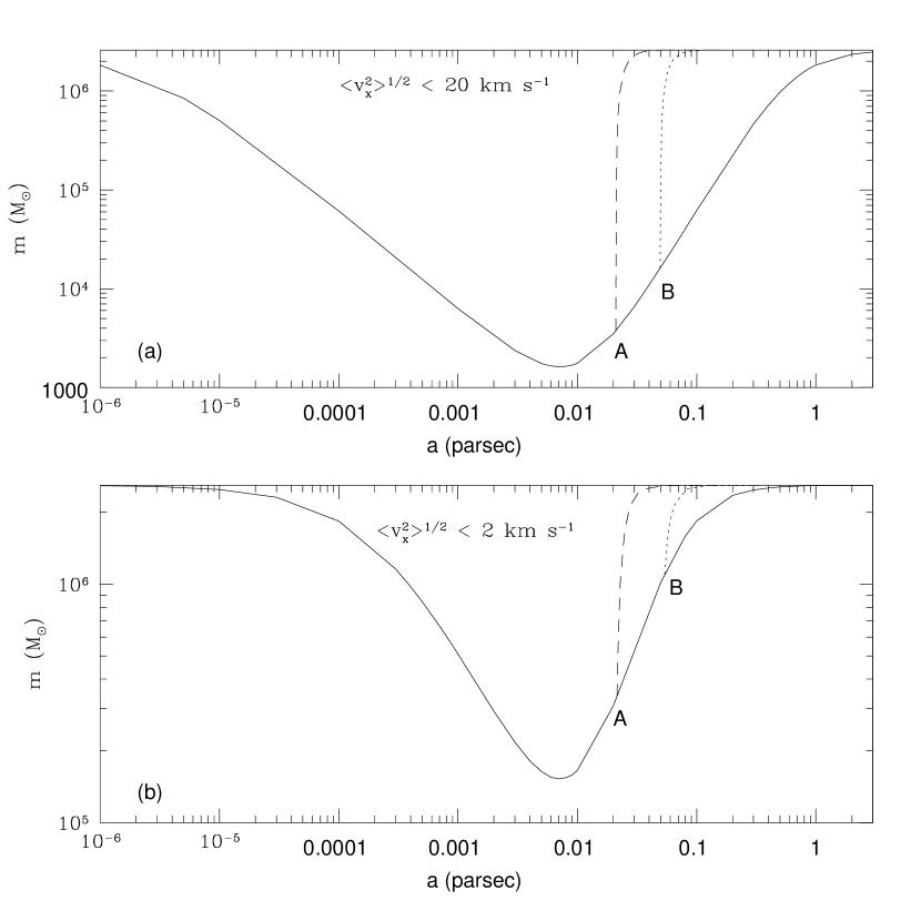
Figure 4: The region above the solid line in the upper panel denotes the allowed values of $m$, the mass of the putative black hole in the Galactic center Sgr A*, and $a$, the length scale characterizing the cluster of stars (each of mass 1 $M_{\odot}$) surrounding Sgr A*, given that the rms value of one component of the black hole’s velocity is $<$ 20 km s^-1. The region to the right of the dashed line denotes the allowed values of $m$ and $a$ if the evaporation timescale of the cluster, $t_{evap}$, exceeds 1 Gyr, and the region to the right of the dotted line denotes the allowed values if $t_{evap}>$ 10 Gyr. The lower panel is the same as the upper panel, except that the rms value of one component of the black hole’s velocity is now assumed to be $<$ 2 km s^-1.

where $<v_{x}^{2}>_{max}$ is the maximum mean squared speed of one component of the black hole’s velocity. We can now set $\langle v_{x}^{2}\rangle_{max}^{1/2}\sim 20$ km s^-1 to get an approximate lower limit on $m$, assuming that $m_{\star}\sim 1M_{\odot}$. This relation is plotted in Figure 4(a) for various values of $a$, the scale length parameter of the Plummer cluster. The mass of the black hole must be given by points lying above the curved solid line. Evidently, this relation implies a lower limit on $m$.

We can derive stricter limits on $m$ by noting, as did Maoz (1998), that the allowed values of $a$ are restricted by the condition that the upper limit of the lifetime of a cluster of stars is its evaporation time, when stars would have escaped from the cluster because of scattering. The evaporation timescale of the cluster should be long enough to make it probable that the cluster be observed at the present epoch. A reasonable assumption is that this timescale, $t_{evap}$, is bounded between the values 1 Gyr and 10 Gyr, the latter being the approximate age of the Galaxy. The evaporation timescale is $t_{evap}\approx 300t_{rh}$, where $t_{rh}$ is the median relaxation time, given by (see, e.g., Maoz 1998, BT)

$$t_{rh}=\frac{0.14N}{\ln(0.4N)}\sqrt{\frac{r_{h}^{3}}{GM}},$$

where $N=M/m_{\star}$ is the number of stars in the cluster (with $M$ given by equation 41), and $r_{h}$ is the system’s median radius; $r_{h}=1.3a$ for the Plummer profile.

Setting $t_{evap}$ = 1 Gyr, we obtain the dashed line in Figure 4(a); $t_{evap}>$ 1 Gyr denotes the region to the right of this line. Hence, the allowed values of $m$ and $a$ lie to the right of this dashed line and above the solid line. The minimum value of $m$ under these assumptions is given by point A at which $m\approx 3.8\times 10^{3}M_{\odot},a\approx 0.021$ pc, and the total mass of the star cluster is $M\approx 3.3\times 10^{7}M_{\odot}$.

If we perform a similar calculation for $t_{evap}>$ 10 Gyr, we obtain the dotted line in Figure 4(a); the minimum value of $m$ is then given by point B at which $m\approx 1.6\times 10^{4}M_{\odot},a\approx 0.049$ pc and $M\approx 3.3\times 10^{8}M_{\odot}$.

Reid et al. (1999) expect further observations to reduce the limit on the peculiar motion of Sgr A* from 20 km s^-1 to 2 km s^-1 over the next few years. Figure 4(b) repeats the above calculations for this limit. The condition $t_{evap}>$ 1 Gyr then gives a new lower limit for $m$ (point A), at which $m\approx 3.4\times 10^{5}M_{\odot},a\approx 0.022$ pc, and $M\approx 3.0\times 10^{7}M_{\odot}$. Point B, the minimum of $m$ if $t_{evap}>$ 10 Gyr, is now characterized by $m\approx 1.1\times 10^{6}M_{\odot},a\approx 0.054$ pc, and $M\approx 2.5\times 10^{8}M_{\odot}$. In the latter case, the attainable lower limit on $m$ will be interestingly close to its upper limit of $M_{R}=2.6\times 10^{6}M_{\odot}$.

7 Summary

In this paper, we have developed a stochastic model to describe the dynamics of a black hole near the center of a dense stellar system. The total force on the black hole is decomposed into a slowly varying part originating from the response of the whole stellar system, and a random, rapidly fluctuating part originating from discrete encounters with individual stars. We have shown that the time scale over which the latter force fluctuates is very short compared with the time scale over which the former changes; hence the justification for the separation of the total force into these two independent components. The slowly varying force itself is approximated as the sum of two contributions: the force on the black hole due to the potential of the whole stellar system and a force of dynamical friction which causes the black hole to decelerate as it moves through the stellar system.

The stochastic force at the position of the black hole is assumed to have a zero average and to be essentially uncorrelated with itself over time scales that are short compared with the characteristic period over which the velocity of the black hole changes considerably, but long enough for many independent fluctuations of the stochastic force to have occurred.

If the stellar system is approximated by a Plummer model, then the problem essentially reduces to describing the Brownian motion of a particle in a harmonic potential. We have shown that after long times, the black hole’s velocity has a zero average and its average location coincides with the center of the stellar potential. However, the root mean squared position and velocity tend towards non-zero values which are independent of time and of the black hole’s initial position and velocity. The steady-state time autocorrelation functions of the position and velocity were shown to be approximately given by damped cosine functions. For a Maxwellian distribution of stars, strict equipartition of kinetic energy between the black hole and the stars is achieved.

The model was completed by solving for the one unknown parameter — the mean squared magnitude of the stochastic force on the black hole — by making use of the close relationship between processes of fluctuation and dissipation, according to which the “heating” by the fluctuating force equals the “cooling” caused by the dissipative force of dynamical friction (the third force on the black hole — the force due to the stellar potential — is conservative).

A Fokker-Planck equation for the diffusion of the probability distribution of the black hole’s position and velocity was developed and solved. The solution implies that in the steady state these variables are distributed independently as Gaussians.

The predictions of the model were tested by comparing with the results of various N-body simulations; the agreement is good, thus justifying the elements of the model. In the simulations, we find possible signs of the existence of weakly damped coherent modes associated with the stellar system (Weinberg 1994). The total force at the origin of the system has a strong Fourier component at the frequency of fundamental oscillations characteristic of the approximately harmonic form of the stellar potential near the center. If we consider the black hole to be a test particle affected by such a force, then the autocorrelation functions of the black hole’s position and velocity would be found not to damp with the time lag, but to persist; the results of simulation do indeed show the presence of such oscillations at very low amplitude for arbitrarily long time lags.

Finally, we applied the results of the model to Sgr A*. Observational limits on the peculiar motion of Sgr A* were used to obtain a lower limit on its mass, under the assumption that it is localized near the center of a system of equal mass stars distributed according to the Plummer model. More stringent limits were then deduced by requiring that the evaporation timescale of the cluster of stars be larger than 1 Gyr.

The Plummer model is a reasonable choice for the black hole problem considered here since it results in a separable system of linear stochastic differential equations; it is not clear that arbitrary potential-density pairs would give equations that are similarly tractable. In particular, what would happen in the case of black holes at the centers of galaxies if those are described by singular power-law density profiles? A simple-minded generalization of our method would not necessarily work (for example, because of possible divergences in the distribution function). However, we believe that our model captures the qualitative features of more complicated situations for two related reasons. First, we note that the Plummer model is not an equilibrium solution for a cluster of stars with a black hole present (see, e.g., Huntley & Saslaw 1975 and Saslaw 1985); even in non-singular models such as the Plummer model, the black hole ultimately induces a density cusp. We have ignored this complication in our model and found that the model nevertheless provides a good description of detailed numerical simulations. Second, the black hole tends to carry its cusp of bound stars with it as it moves around; thus, it is as if a black hole of a somewhat larger effective mass were moving in a background consisting of unbound stars. With the cusp effectively removed, the density profile of this background would be flat near the center. Since the restoring force and dynamical friction are provided mainly by the unbound stars, we believe that the essential components of our model are still valid. (For similar reasons – see §5 for details – the fact that our simulations use a fixed stellar potential is not expected to alter our conclusions.) We have carried out numerical simulations for the case of a particular density profile with a singularity, namely the Hernquist (1990) model. We find that the qualitative results are similar to those described here. In particular, the early-time autocorrelation functions of the black hole’s force and velocity continue to be described well by damped cosine functions of fixed frequency. The detailed characterization of the black hole behavior in terms of the model parameters is different, and requires a more careful calculation.

We thank G. Quinlan for providing the simulation code, S. Tremaine for enlightening discussions and a careful reading of the manuscript, and M.J. Reid and G. Rybicki for useful discussions. We also thank the editor, Ethan Vishniac, for his helpful advice. This work was supported in part by NASA grants NAG 5-7039, 5-7768, and by NSF grants AST-9900877, AST-0071019 (for AL).

Figure 1: Results from a simulation of a black hole of mass $m=0.01$ in a Plummer model of total mass $M=1$ and $N=100,000$ stars. The evolution of the $x$-components of the black hole’s position and velocity are shown from $t=0$ to $t=100$. The third panel shows the autocorrelation function of $x$ for time lags from $T=0$ to $T=20$. The solid line is the autocorrelation function obtained from the simulation, and the broken line is that predicted by our model.

Figure 2: Results from simulations of a black hole of mass $m=0.01$ in a Plummer model of total mass $M=1$ and $N=\,$ 12,500, 25,000, 50,000 and 100,000 stars. The panels show the root mean squared values of the $x$-components of the black hole’s position and velocity. The crosses show the results obtained from the simulations, and the solid lines are the values predicted by our model. In each case, the simulation was stopped at time $t=600$.

Figure 3: Results from a simulation of a black hole of mass $m=0.01$ in a Plummer model of total mass $M=1$ and $N=100,000$ stars. The distributions of the $x$-components of the black hole’s position and velocity are shown as histograms. The solid lines show the corresponding bin values according to the analytic model of this paper.

References

- (1)
- (2) Aarseth, S.J. 1994, Direct Methods for N-Body Simulations, in Galactic Dynamics and N-Body Simulations, eds. G. Contopoulos, N.K. Spyrou & L. Vlahos (Springer-Verlag)
- (3)
- (4) Bahcall, J.N. & Wolf, R.A. 1976, ApJ 209, 214
- (5)
- (6) Bekenstein, J.D. & Maoz, E. 1992, ApJ 390, 79
- (7)
- (8) Binney, J., & Tremaine, S. 1987, Galactic Dynamics (Princeton: Princeton Univ. Press) (BT)
- (9)
- (10) Chandrasekhar, S. 1943a, Rev. Mod. Phys. 15, 1
- (11)
- (12) Chandrasekhar, S. 1943b, ApJ 97, 255
- (13)
- (14) Chandrasekhar, S. 1944a, ApJ 99, 47
- (15)
- (16) Chandrasekhar, S. 1944b, ApJ 99, 54
- (17)
- (18) Cohen, L. 1975, in Hayli, A., ed. Proc. IAU Symp. 60, Dynamics of Stellar Systems (Reidel, Dordrecht), p. 33
- (19)
- (20) Eckart, A., & Genzel, R. 1997, MNRAS 284, 576
- (21)
- (22) Gebhardt, K. et al. 2001, astro-ph/0107135
- (23)
- (24) Ghez, A.M., Klein, B.L., Morris, M. & Becklin, E.E. 1998, ApJ 509, 678
- (25)
- (26) Ghez, A.M., Morris, M., Becklin, E.E., Tanner, A., & Kremenek, T. 2000, Nature 407, 349
- (27)
- (28) Greenhill, L.J., Jiang, D.R., Moran, J.M., Reid, M.J., Lo, K.Y. & Claussen, M. J. 1995, ApJ 440, 619
- (29)
- (30) Hernquist, L. 1990, ApJ 356, 359
- (31)
- (32) Huntley, J.M. & Saslaw, W.C. 1975, ApJ 199, 328
- (33)
- (34) Kormendy, J. & Richstone, D. 1995, Annu. Rev. Astron. Astrophys. 33, 581
- (35)
- (36) Lin, D.N.C. & Tremaine, S. 1980, ApJ 242, 789
- (37)
- (38) Lynden-Bell, D. 1969, Nature, 223, 690
- (39)
- (40) Maoz, E. 1993, MNRAS 263, 75
- (41)
- (42) Maoz, E. 1998, ApJ 494, L181
- (43)
- (44) Mathur, S.D. 1990, MNRAS 243, 529
- (45)
- (46) Melia, F. & Falcke, H. 2001, Annu. Rev. Astron. Astrophys. 39 (in press)
- (47)
- (48) Merritt, D. 2001, astro-ph/0012264 v.2
- (49)
- (50) Miller, R.H. 1992, Am. Sci. 80, 153
- (51)
- (52) Miller, R.H. & Smith, B.F. 1992, ApJ 393, 508
- (53)
- (54) Nelson, R.W. & Tremaine, S. 1999, MNRAS 306, 1
- (55)
- (56) Quinlan, G.D. & Hernquist, L. 1997, NewA 2, 533
- (57)
- (58) Rees, M. 1984, ARA&A, 22, 471
- (59)
- (60) Reid, M.J., Readhead, A.C.S., Vermeulen, R.C. & Treuhaft, R.N. 1999, ApJ 524, 816
- (61)
- (62) Salpeter, E. E. 1964, ApJ, 140, 796
- (63)
- (64) Saslaw, W.C. 1985, Gravitational Physics of Stellar and Galactic Systems (Cambridge: Cambridge Univ. Press)
- (65)
- (66) Tremaine, S. & Weinberg, M.D. 1984, MNRAS 209, 729
- (67)
- (68) Wang, M.C., & Uhlenbeck, G.E. 1945, Rev. Mod. Phys. 17, 323
- (69)
- (70) Weinberg, M.D. 1994, ApJ 421, 481
- (71)
- (72) Weinberg, M.D. 1986, ApJ 300, 93
- (73)
- (74) Zel’dovich, Ya. B. 1964, Soviet Physics Doklady, 9, 195
- (75)