Evolutionary Binary Sequences for Low- and Intermediate-Mass X-Ray Binaries

Abstract

We present the results of a systematic study of the evolution of low- and intermediate-mass X-ray binaries (LMXBs and IMXBs). Using a standard Henyey-type stellar-evolution code and a standard model for binary interactions, we have calculated 100 binary evolution sequences containing a neutron star and a normal-type companion star, where the initial mass of the secondary ranges from 0.6 to 7$\,M_{\odot}$ and the initial orbital period from $\sim 4\,$hr to $\sim 100\,$d. This grid of models samples the entire range of parameters one is likely to encounter for LMXBs and IMXBs. The sequences show an enormous variety of evolutionary histories and outcomes, where different mass-transfer mechanisms dominate in different phases. Very few sequences resemble the classical evolution of cataclysmic variables, where the evolution is driven by magnetic braking and gravitational radiation alone. Many systems experience a phase of mass transfer on a thermal timescale and may briefly become detached immediately after this phase (for the more massive secondaries). In agreement with previous results (Tauris & Savonije 1999), we find that all sequences with (sub-)giant donors up to $\sim 2\mbox{$\,M_{\odot}$}$ are stable against dynamical mass transfer. Sequences where the secondary has a radiative envelope are stable against dynamical mass transfer for initial masses up to $\sim 4\mbox{$\,M_{\odot}$}$. For higher initial masses, they experience a delayed dynamical instability after a stable phase of mass transfer lasting up to $\sim 10^{6}\,$yr. Systems where the initial orbital period is just below the bifurcation period of $\sim 18\,$hr evolve towards extremely short orbital periods (as short as $\sim 10\,$min). For a 1$\,M_{\odot}$ secondary, the initial period range that leads to the formation of ultracompact systems (with minimum periods less than $\sim 40\,$min) is 13 to 18 hr. Since systems that start mass transfer in this period range are naturally produced as a result of tidal capture, this may explain the large fraction of ultracompact LMXBs observed in globular clusters. The implications of this study for our understanding of the population of X-ray binaries and the formation of millisecond pulsars are also discussed.

Submitted to ApJ

1 Introduction

Low-mass X-ray binaries (LMXBs) were discovered nearly 40 years ago, and there are now $\sim 100$ known in the Galaxy. Based on their short orbital periods of $\lesssim 10\,$d and the absence of luminous companion stars, it is generally inferred that the donor stars in these systems are typically low-mass stars (i.e., $\lesssim 1M_{\odot}$). However, to-date Cyg X-2 provides the only case in which a low mass for the donor star has actually been confirmed dynamically (Casares, Charles, & Kuulkers 1998; Orosz & Kuulkers 1998). Nonetheless, a fairly compelling picture of LMXBs has emerged over the years, wherein a low-mass donor star, of varying evolutionary states, transfers mass through the inner Lagrange point to a neutron star (Lewin, van Paradijs, & van den Heuvel 1995). Only relatively recently, however, has attention been focused on the possibility that many, or perhaps most, of the current LMXBs descended from systems with intermediate-mass donor stars (hereafter IMXBs).

It has long been conventional wisdom that, if the donor star in an X-ray binary is significantly higher in mass than the accreting neutron star, mass transfer would be unstable on a dynamical timescale, and therefore such systems would not survive. The first systematic study which indicated that such a view was too simplistic was carried out by Pylyser & Savonije (1988, 1989), who considered compact binaries with initial donor masses up to $2\,M_{\odot}$ and initial orbital periods of $\lesssim 2\,$d. Tauris & Savonije (1999) extended this work to show that, even if the donor star is a (sub-)giant, dynamical mass transfer is avoided provided that the initial donor mass is $\lesssim 2\,M_{\odot}$.

More recent theoretical work in trying to understand the origin of the “LMXB” Cyg X-2 and, in particular, the high intrinsic luminosity of the donor star indicates that the mass of the donor must originally have been substantially larger ($\sim 3.5\,M_{\odot}$) than the current value of $\sim 0.6\mbox{$\,M_{\odot}$}$ (King & Ritter 1999; Podsiadlowski & Rappaport 2000). The case of Cyg X-2 is particularly important since it provides direct observational evidence that, even when the mass-transfer rate exceeds the Eddington rate by several orders of magnitude, such intermediate-mass systems can survive this phase of high mass-transfer by ejecting most of the transferred mass and subsequently mimick LMXBs. Independently, Davies & Hansen (1998) have suggested that IMXBs may be the progenitors of recycled pulsars in globular clusters. All of these recent developments have led to a resurgence in interest in IMXBs (also see Kolb et al. 2000; Tauris, van den Heuvel, & Savonije 2000).

In order to approach this problem in a more systematic way, we have carried out binary stellar evolution calculations which cover a broad grid of starting binary parameters, specifically the mass of the donor star, $M_{2}$, and the orbital period at the start of the mass-transfer phase, $P_{\rm orb}$. At fixed $M_{2}$, the value of initial orbital period effectively determines the evolutionary state of the donor star. This library of models comprises 17 different donor-star masses between $0.6\,M_{\odot}$ and $7\,M_{\odot}$, and up to 8 different evolutionary states (or, alternatively, values of $P_{\rm orb}$). The initial orbital periods span the range from $\sim 4$ hours to 100 days. The starting parameter values associated with this library of models are summarized in Figure 1. In this figure we show the initial binary parameters in a Hertzsprung-Russell (H-R) diagram for the companion star. Evolutionary tracks for stars of the same mass, but which evolve as single stars are superposed for reference. Contours of constant initial orbital period for the case of Roche lobe overflow onto a neutron star of $1.4\,M_{\odot}$ are also included.

In our binary evolution models, once mass transfer has commenced, it is sustained by either (i) systemic angular-momentum losses (e.g., magnetic braking or gravitational radiation), or (ii) expansion of the donor star due to nuclear and/or thermal evolution. The mass transfer may proceed on any of the timescales implicit in the mechanisms listed above, or may in fact proceed on a dynamical timescale under certain conditions. All of these are explored in detail in this study.

During the mass transfer phases, these objects will generally appear as X-ray sources (possibly LMXBs, IMXBs). These sources could be steady or transient, depending on the size and temperature of the accretion disk and on the mass transfer rate through the disk. At the end of the mass-transfer phase, many of these systems will become binary radio pulsars, wherein the neutron star has been spun up to high rotation rates by the accretion of matter.

One of the main objectives of this study is to provide a library of models that covers the whole range of parameters for LMXBs and IMXBs using a self-consistent set of binary calculations and to discuss the various physical phenomena encountered in the process. In a subsequent study (Pfahl, Podsiadlowski, & Rappaport 2001), we will use this library to study the population of LMXBs and IMXBs as a whole by integrating them into a binary population synthesis code and by comparing the results with the observed population.

In §2 of this paper we describe in detail the stellar evolution code and the binary model used in this study. In §3 we discuss the various types of binary sequences encountered and compare them to previous studies. In §4 we consider the end products of this evolution and present a new case study for the formation of ultracompact X-ray binaries. Finally in §5 and 6, we discuss the implications of these results for the population of X-ray binaries and the formation of binary millisecond pulsars.

2 Binary Calculations

2.1 The Stellar-Evolution Code

All calculations were carried out with an up-to-date, standard Henyey-type stellar evolution code (Kippenhahn, Weigert, & Hofmeister 1967), which uses OPAL opacities (Rogers & Iglesias 1992) complemented with those from Alexander & Ferguson (1994) at low temperatures. We use solar metallicity ($Z=0.02$), a mixing-length parameter $\alpha=2$ and assume 0.25 pressure scale heights of convective overshooting from the core, following the recent calibration of this parameter by Schröder, Pols, & Eggleton (1997) and Pols et al. (1997). To include the effects of pressure ionization in the equation of state, which is important for low-mass stars, we adopted the thermodynamically self-consistent formalism of Eggleton, Faulkner, & Flannery (1973) and calibrated the continuum depression term so that our models for single stars compare well with the detailed models of Baraffe et al. (1998). Our models agree with these models typically within a few per cent in radius (for masses as low as $0.1\,M_{\odot}$), although their luminosities may differ by as much as $\sim 20$ per cent. This may be due, in part, to the fact that we required a helium abundance of 0.295 for $\alpha=2$ to produce a good solar model at the present age of the Sun, as compared to their value of 0.282 for $\alpha=1.9$. Our single-star models become fully convective at a mass of $0.351\,M_{\odot}$.

2.2 The Binary-Evolution Code

Each of the binaries initially consists of a neutron-star primary with an initial mass $M_{1}=1.4\,M_{\odot}$ and a normal-type secondary of mass $M_{2}$. The effective radius of the Roche lobe, $R_{\rm L}$, is calculated with the formula of Eggleton (1983),

$$R_{\rm L}=a\,{0.49\,q^{-2/3}\over 0.6\,q^{-2/3}+\ln(1+q^{-1/3})},$$ (1)

where $a$ is the orbital separation and $q=M_{1}/M_{2}$ the mass ratio of the binary components. To calculate the mass-transfer rate, $\dot{M}$, we adopted the prescription of Ritter (1988),

$$\dot{M}=\dot{M}_{0}\,e^{R-R_{\rm L}\over H_{\rm p}},$$ (2)

where $R$ is the radius of the secondary and $H_{\rm p}$ the pressure scale height at its surface. The constant $\dot{M}_{0}$ is calculated according to the model of Ritter (1988). The solution of this equation requires an iteration in the stellar models. We follow the method described by Braun (1997), which uses a combined secant/bisection method (the Brent method; see, e.g., Press et al. 1992).

Angular-momentum loss due to gravitational radiation is calculated according to the standard formula (Landau & Lifshitz 1959; Faulkner 1971),

$${d\,\ln J_{\rm GR}\over dt}=-{32\over 5}\,{G^{3}\,c^{5}}{M_{1}M_{2}(M_{1}+M_{2})\over a^{4}},$$ (3)

where $G$ and $c$ are the gravitational constant and vacuum speed of light, respectively. To calculate the angular-momentum loss due to magnetic braking, we use the prescription of Rappaport, Verbunt, & Joss (1993) (their eq. 36 with $\gamma=4$), which is based on the magnetic-braking law of Verbunt & Zwaan (1981),

$${d\,J_{MB}\over dt}=-3.8\times 10^{-30}\,M_{2}\,R^{4}\,\omega^{3}\mbox{\ \ \rm dyn\,\,cm}.$$ (4)

In this equation $\omega$ is the angular rotation frequency of the secondary, assumed to be synchronized with the orbit. We only include full magnetic braking if the secondary has a sizable convective envelope, taken to be at least $2\,\%$ in mass (see also Pylyser & Savonije 1988). For secondaries with convective envelopes smaller than $2\,\%$, we reduce the efficiency of magnetic braking by an ad hoc factor $\exp\{-0.02/q_{\rm conv}+1\}$, where $q_{\rm conv}$ is the fractional mass of the convective envelope. We also assume that magnetic braking stops when the secondaries become fully convective (Rappaport et al. 1983; Spruit & Ritter 1983).

We do not follow the tidal evolution before the onset of mass transfer (see, e.g., Witte & Savonije 2001), but start our binary sequences assuming that the systems have already circularized when the secondaries are close to filling their Roche lobes; to be precise we start our calculations when the mass transfer rate as given by equation (2) is $\sim 10^{-14}\,M_{\odot}\,$yr^-1.

For each sequence, we need to specify what fraction, $\beta$, of the mass lost by the donor is accreted by the neutron star and the specific angular momentum of any matter that is lost from the system. We scale the latter with the specific orbital angular momentum of the neutron star, i.e., assume that the angular momentum loss due to mass loss from the system is given by

$${d\,J_{ML}\over dt}=-\alpha\,(1-\beta)\,a_{1}^{2}\,\omega\,\dot{M},$$ (5)

where $\alpha$ is an adjustable parameter and $a_{1}$ the orbital radius of the neutron star. The change of the orbital separation due to the systemic mass loss alone can be calculated analytically according to

$${a^{1}\over a^{0}}=\left({M_{2}^{1}\over M_{2}^{0}}\right)^{C_{1}}\,\left({M_{1}^{1}\over M_{1}^{0}}\right)^{C_{2}}\,\left({M_{1}^{1}+M_{2}^{1}\over M_{1}^{0}+M_{2}^{0}}\right)^{C_{3}},$$ (6)

where superscripts 0 indicate initial values and superscripts 1 final values and where the exponents are given by

$$C_{1} = -2$$

$$C_{2} = -2-2\alpha\,(1-\beta)/\beta$$ (7)

$$C_{3} = 1-2\alpha.$$

When $\beta=0$, equation (6) has to be replaced by

$${a^{1}\over a^{0}} = \left({M_{2}^{1}\over M_{2}^{0}}\right)^{C_{1}}\,\,\left({M_{1}+M_{2}^{1}\over M_{1}+M_{2}^{0}}\right)^{C_{3}}\,$$ (8)

$$\hskip 28.45274pt\times\exp\left\{2\alpha\,\left({M_{2}^{1}-M_{2}^{0}\over M_{1}}\right)\right\}.$$

In all of our sequences, we take $\alpha$ to be 1, which implicitly assumes that all the mass lost from the system is lost from the neighborhood of the neutron star (or its accretion disk), and set $\beta$, somewhat arbitrarily, equal to 0.5. In addition, we limit the maximum accretion rate onto the neutron star to the Eddington accretion rate, taken to be $\dot{M}=2\times 10^{-8}\mbox{$\,M_{\odot}\,$yr${}^{-1}$}$ and kept constant throughout each run. In our calculations with relatively massive secondaries, the mass-transfer rate can exceed the Eddington accretion rate by many orders of magnitude. Most of this excess mass must be lost from the system, as the case of Cyg X-2 has demonstrated. This mass loss may, for example, occur in the form of a relativistic jet from the accreting neutron star or a radiation-pressure driven wind from the outer parts of the accretion disk (see, e.g., King & Begelman 1999). Evidence for both of these processes is seen in the X-ray binary SS 433 (Blundell et al. 2001), the only system presently known to be in an extreme super-Eddington mass-transfer phase.

Since the pressure scale height at the surface of the donor is generally a small fraction of the stellar radius (often as low as $\sim 10^{-4}\,R$), the calculation of the mass-transfer rate according to equation (2) requires that the radius of the star be calculated to very high precision. To avoid discontinuous changes in radius and hence $\dot{M}$, it is important that the chemical profile of the initial star is well resolved and that abrupt changes in the surface abundances (for example, as a result of dredge-up) are avoided. To calculate mass loss efficiently, we introduced a moving mesh in the outermost 5 % of the mass of the star. We also assumed that the outermost $10^{-4}$ of the envelope mass of the donor star was in thermal equilibrium. This is necessary since in each time step we typically take off a much larger fraction of the mass of the star and since the structure variables often change by a large factor in this outermost layer. It is also justified since the thermal timescale of this layer is much shorter than any mass-loss timescale encountered in this study. (We have extensively tested that our results are not sensitive to these assumptions, at least for the mass-loss rates obtained, where we generally limited the maximum mass-loss rate to $10^{-4}\,M_{\odot}\,$yr^-1.)

Despite of these precautions, our calculated mass-loss rates are occasionally subject to numerical oscillations. These tend to be almost negligible for stars with radiative envelopes (typically less than a few percent), but can be several 10’s of per cent for stars with convective envelopes and occasionally much larger for evolved giants (in particular during dredge-up phases). We note that, in all of the plots of $\dot{M}$ presented in this paper, these oscillations, which do not affect the secular evolution of the systems, have been averaged out.

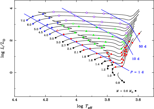
Figure 1: Overview of the initial parameters of the secondaries in the Hertzsprung-Russell (H-R) diagram for the 100 binary evolution sequences in the study. The thin solid curves represent evolutionary tracks of single stars with the masses as indicated. The thick solid curves show the orbital periods of systems when the secondaries start to fill their Roche lobes at the particular positions along the evolutionary tracks (assuming a mass for the primary of 1.4$\,M_{\odot}$, as appropriate for a neutron star). The symbols are placed at the initial positions of the secondaries in our sequences, where the type of symbol indicates the final fate of the systems (squares: ultracompact systems; circles: He white dwarfs; triangles: HeCO white dwarfs; filled stars: delayed dynamical mass transfer; unfilled stars: dynamical mass transfer; in cases where it is not clear whether the system experiences a dynamical instability, symbols are plotted on top of a star).

2.3 Tests and Comparisons

To test our binary evolution code, we chose to calculate the standard evolution of a cataclysmic variable (CV), initially consisting of a white dwarf of $0.6\,M_{\odot}$ and a secondary of $0.8\,M_{\odot}$ (here we assumed that all of the mass transferred from the secondary was lost from the system). In this calculation, the system experienced a period gap between 2.4 and 3.1 hr, somewhat smaller than the observed gap (Ritter & Kolb 1998), but consistent with previous results for our adopted magnetic-braking law (Rappaport, Verbunt, & Joss 1983). The minimum period in this calculation was 75 min, somewhat longer than the minimum period found in the most detailed studies of CVs (see, e.g., Kolb & Baraffe 1999; Howell, Nelson, & Rappaport 2001).

We also compared our calculations to other recent similar binary calculations by a number of different authors, in particular the calculations by Pylyser & Savonije (1988, 1989); Han, Tout, & Eggleton (2000); Langer et al. (2000); Kolb et al. (2000); Tauris et al. (2000). For comparable models, we generally find excellent agreement between our calculations and the calculations of these authors. The only significant discrepancy to note is the early case B calculation for Cyg X-2 by Kolb et al. (2000), where the secondary has an initial mass of 3.5$\,M_{\odot}$ and has just evolved off the main sequence at the beginning of mass transfer. While our early-case B model (see Podsiadlowski & Rappaport 2000) is in excellent agreement with a similar calculation by Tauris et al. (2000), in the Kolb et al. model, the early super-Eddington phase is much longer, and as a consequence the mass-transfer rate in the subsequent slower phase about an order of magnitude lower than in our model. We do not know the reason for this discrepancy, whether it has to do with the treatment of mass loss at these very high rates ($\sim 10^{-5}\,M_{\odot}\,$yr^-1) or whether it is caused by differences in the structure of the initial models (U. Kolb 2000, private communication). For example Kolb et al. (2000) do not include convective overshooting in their calculations; this produces a different chemical profile just outside the hydrogen-exhausted core, which may affect the evolution of the secondary (the evolutionary track of their secondary in the H-R diagram is indeed quite different). Until this discrepancy is resolved, we note that there is some uncertainty in the modeling of these systems with extreme mass-transfer rates.

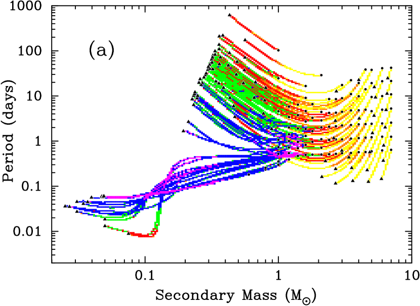
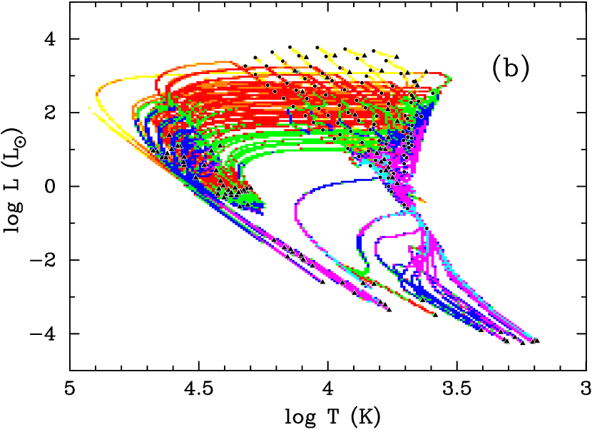
Figure 2: Time-weighted evolutionary tracks for the 100 binary sequences in the secondary mass – orbital period plane (panel a) and for the secondaries in the H-R diagram (panel b). The color of the tracks indicate how much time systems spend in a particular rectangular pixel in the diagrams (from short to long: yellow, orange, red, green, blue, magenta, cyan). The minimum time displayed was chosen to be 100 yr, and the maximum time in each of the panels is $\sim 9.5\,$Gyr. The 7 colors are distributed evenly in $\log t$ between these times. Circles and triangles mark the starting and final points in the sequences, respectively.

3 Results of Binary Calculations

Altogether we carried out 100 binary stellar evolution calculations with initial secondary masses ranging from $0.6\,M_{\odot}$ to $7\,M_{\odot}$ and covering, in a fairly uniform manner, all evolutionary stages likely to be encountered for LMXBs/IMXBs, with orbital periods from 4 hr to 100 d (see Fig. 1). In Figure 2 we present the evolutionary tracks of these calculations both in a secondary mass – orbital period diagram ($\log M_{2}\,$–$\,\log P_{\rm orb}$; Fig. 2a) and in a traditional Hertzsprung-Russell (H-R) diagram (Fig. 2b), where the color coding indicates how much time a system spends in a particular region of the diagrams. What these figures do not show very well, however, is the actual variety in these sequences. Some 70 of the 100 sequences are qualitatively different with respect to the importance and the order of different mass-transfer driving mechanisms, the occurrence of detached phases, the final end products, etc. Indeed there are very few sequences that resemble the classical CV evolution where mass-transfer is driven solely by gravitational radiation and magnetic braking. Instead of presenting all of these sequences in detail, we will discuss the various physical phenomena encountered and illustrate them with particular evolutionary sequences. In the appendix we present the key characteristics of each sequence in tabular form.

As Figure 2 shows, the sequences can be broadly divided into three classes: (1) and (2) systems evolving to long periods and short periods, respectively, and (3) more massive systems experiencing dynamical mass transfer and spiral-in (the short yellow tracks). The systems evolving towards short and long orbital periods are separated by the well-known bifurcation period that has been studied by several authors in the past (see, in particular, Tutukov et al. 1985; Pylyser & Savonije 1988; Ergma 1996; Ergma & Sarna 1996). For our binary model, the bifurcation period occurs around 18 hr for a 1$\,M_{\odot}$ model (see §4.2 for a systematic case study). This implies that all 1$\,M_{\odot}$ models that start mass transfer on or just off the main sequence evolve towards short periods, while for the more massive secondaries only relatively unevolved secondaries do so (see Fig. 1), in agreement with the findings of Pylyser & Savonije (1988). However, the value of the bifurcation period and the behavior of the evolutionary tracks near the bifurcation period is very sensitive to the model assumptions, in particular the magnetic-braking law (Pylyser & Savonije 1988 and § 4.2) and the assumptions about mass loss from the system (Ergma 1996; Ergma & Sarna 1996). Because of the strong divergence of tracks below and about the bifurcation period, one would expect very few systems with final orbital periods near the bifurcation period (Pylyser & Savonije 1988) unless a system started its evolution very close to it initially (Ergma 1996).

Figure 2 also shows that, for the more massive systems, the initial evolution is very rapid. As a direct consequence, very few systems should be observable in this early rapid phase, and X-ray binaries are most likely to have a relatively low-mass secondary when they are observed at the present epoch, even if they had a much more massive companion initially.

3.1 Low-Mass Models and the Role of Magnetic Braking

If the secondary is a relatively unevolved low-mass star initially (with mass $\lesssim 1\mbox{$\,M_{\odot}$}$), the only important mechanisms driving mass transfer are systemic angular-momentum losses due to magnetic braking and gravitational radiation. This type of evolution is similar to the classical evolution of CVs. The systems evolve towards shorter periods, may experience a period gap when magnetic braking stops being effective (when the secondary becomes fully convective) and ultimately reach a minimum period just before hydrogen burning is extinguished (Paczyński & Sienkiewicz 1981; Rappaport, Joss, & Webbink 1982). Beyond the period minimum (which depends on the evolutionary stage of the initial model), the secondaries follow the mass-radius relation for degenerate stars and the systems will expand, driven by gravitational radiation alone.

This classical CV-like evolution is illustrated in Figures 3 and 4 for three binary sequences with initial secondaries of 1$\,M_{\odot}$ and different evolutionary stages (at the beginning, the middle and the end of the main sequence). Figure 3 shows the evolution of orbital period and mass-transfer rate as a function of time since the beginning of mass transfer (the evolutionary tracks of the secondaries in the H-R diagram are shown in Fig. 4). These calculations serve to illustrate several points, already found in previous studies (see, in particular, Pylyser & Savonije 1989). The maximum mass-transfer rate is of order a few $10^{-9}\mbox{$\,M_{\odot}\,$yr${}^{-1}$}$, where the more evolved secondaries experience the lower rates. Indeed, this behavior is also often found for more massive secondaries, where the somewhat evolved stars generally tend to be more stable than the unevolved ones. The period gap for the calculation with the initially unevolved secondary is substantially smaller (2.8 to 3.1 hr) than the period gap for a similar CV calculation where the secondary is a white dwarf of 0.6$\,M_{\odot}$ (2.4 to 3.1 hr). While the donor stars become fully convective at more-or-less the same orbital period, they have different masses, 0.336$\,M_{\odot}$ and 0.273$\,M_{\odot}$, respectively, since the donor in the LMXB case is not as much out of thermal equilibrium as in the CV case (the magnetic-braking timescale is a factor of $\sim 2.2$ longer in the LMXB case, while the gravitational-radiation timescale is a factor of $\sim 2.6$ shorter; cf eqs. 3 and 4).

The location and the extent of the period gap decreases for the more evolved systems and completely disappears for the most evolved one. The reason is that the more evolved secondaries become fully convective at a lower mass, which implies a shorter orbital period for the system; but at shorter orbital periods, the timescales for angular-momentum loss due to gravitational radiation and magnetic braking become more comparable, hence producing a smaller gap. Since this type of evolution is similar to the classical CV evolution, it has the obvious implication, as emphasized by Pylyser & Savonije (1989), that the vast majority of secondaries in CVs have to be essentially unevolved initially to prevent the appearance of too many systems in the observed period gap (Ritter & Kolb 1998).

The minimum periods decrease for the more evolved systems, again consistent with previous studies (see §4.2 for further discussion). The system that started mass transfer Figure 3: Evolution of orbital period (upper panel) and mass-transfer rate (lower panel) as a function of time since the beginning of mass transfer (with arbitrary offset) for three binary sequences with an initial secondary of 1$\,M_{\odot}$ and three evolutionary phases (beginning [blue], middle [green] and end of main-sequence phase [red]; from down to up in the upper panel and up to down in the lower panel at early times). The least evolved system experiences a period gap between 2.8 and 3.1 hr and attains a minimum period of 83 min, the model in the middle of the main sequence has a period gap between 2.2 and 2.4 hr and a period minimum of 80 min, while the most evolved system experiences no period gap and has a minimum period of 48 min.

when the secondary had just completed hydrogen burning in the center attains a minimum period of 48 min (note the spike in $\dot{M}$ near the minimum period in this case).

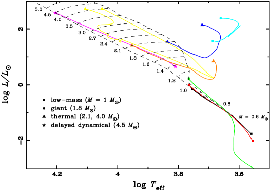
Figure 4: Evolutionary tracks of the secondaries in the H-R diagram for the illustrative sequences discussed in the text. The symbols at the end points of the sequences identify the models (squares: low-mass models [§3.1]; triangles: thermal mass-transfer models [§3.2]; circles: evolution on the giant branch [§3.3]; delayed dynamical instability [§3.3]). The sequences are terminated either near the period minimum (‘low-mass’), at the onset of dynamical instability (‘delayed dynamical’), or at the end of mass transfer (‘giant’ and ‘thermal’). The grid of dashed curves indicates the position of the main-sequence band and the evolutionary tracks for single stars of the masses as indicated.

3.2 Thermal timescale mass transfer

If the donor is initially more massive than the accretor, the Roche lobe radius generally shrinks. If this radius is less than the thermal equilibrium radius of a star of the same mass, the secondary can no longer stay in thermal equilibrium and mass transfer will proceed on a thermal timescale or, in more extreme cases, on a dynamical timescale (see § 3.3; for general reviews of thermal timescale mass transfer see, e.g., Paczyński 1970; Ritter 1996, and for other recent discussions Di  Stefano et al. 1997; Langer et al. 2000; King et al. 2001). It is customary to analyze the stability of mass transfer in terms of mass–radius exponents where

$$\xi_{\rm eq}=\left({d\ln R\over d\ln M}\right)_{\rm eq},\,\,\,\xi_{\rm RL}=\left({d\ln R\over d\ln M}\right)_{\rm RL}$$

$$\mbox{and\,\,\,}\xi_{\rm ad}=\left({d\ln R\over d\ln M}\right)_{\rm ad}$$ (9)

define, respectively, the mass–radius exponents for stars in thermal equilibrium, for the Roche-lobe, and for stars losing mass adiabatically. If the Roche-lobe radius shrinks more rapidly than the adiabatic radius (i.e., if $\xi_{\rm RL}>\xi_{\rm ad}$), then there is no hydrostatic solution for which the secondary can fill its Roche lobe (as defined by eq. 2) and mass transfer will proceed on a dynamical timescale (see § 3.3). The case where mass transfer is dynamically stable, but occurs on a thermal timescale is given by the inequalities $\xi_{\rm ad}>\xi_{\rm RL}>\xi_{\rm eq}$.

For stars with radiative envelopes, $\xi_{\rm ad}$ is generally very large initially, and in most situations much larger than $\xi_{\rm RL}$ ($\xi_{\rm RL}$ generally depends on the mass ratio and any changes in orbital separation due to the transfer of mass and systemic mass and angular momentum losses; see, e.g., Rappaport et al. 1983). To illustrate this, we show approximate adiabatic mass–radius exponents, $\xi_{\rm ad}$, in Figure 5 for stars with initial masses from 1.2 – 2.2$\,M_{\odot}$ and the corresponding mass–radius relations (these were obtained by taking mass off these stars at a high constant rate of $10^{-5}\mbox{$\,M_{\odot}\,$yr${}^{-1}$}$). The large initial values for $\xi_{\rm ad}$ imply that the star has to lose very little mass to shrink significantly. This simply reflects the fact that, in radiative stars, a large fraction of the envelope (in radius) contains very little mass (for example, in an unevolved 2.1$\,M_{\odot}$ star, the outer 40 % of the radius contains just 1 % of the mass). Once this low-density, high-entropy layer is lost, $\xi_{\rm ad}$ drops dramatically to a value of order 1 and ultimately becomes negative when the convective, flat-entropy core is exposed. From this stage on, the radius of the star increases with further mass loss. Since the whole star expands dramatically in this phase, it will be very underluminous for its mass (since most of the internal luminosity drives the expansion) and nuclear burning will ultimately be turned off because of a dramatic decrease in the central temperature. As long as $\xi_{\rm ad}$ remains larger than $\xi_{\rm RL}$, mass transfer remains dynamically stable. The star, which is undersized for its mass, will expand and try to relax to its equilibrium radius. It is this relaxation of the star on a thermal timescale that gives this mode of mass transfer its name.

A characteristic mass-transfer rate for this phase is often defined by an expression of the form (see, e.g., Rappaport, Di  Stefano, & Smith 1994; Langer et al. 2000)

$$\dot{M}_{\rm th}={(M_{2}^{i}-M_{1}^{i})\over t_{\rm KH}},$$ (10)

where $M_{2}^{i}$ and $M_{1}^{i}$ are the initial masses of the secondary (the mass donor) and the primary, respectively, and $t_{\rm KH}$ is the Kelvin-Helmholtz timescale of the secondary (i.e., the thermal timescale of the whole star),

$$t_{\rm KH}\simeq{GM_{2}^{2}\over 2RL},$$ (11)

Figure 5: Approximate adiabatic mass–radius relations (top panel) and adiabatic mass–radius exponents, i.e., $d\ln R/d\ln M$, (bottom panel) for unevolved stars of masses 1.2, 1.4, 1.6, 1.8, 2.0, and 2.3$\,M_{\odot}$. These were calculated by assuming a constant mass-loss rate of $10^{-5}\mbox{$\,M_{\odot}\,$yr${}^{-1}$}$. At this high rate, the entropy profile, $S(M)$, remains almost unchanged (“adiabatic”).

where $R$ and $L$ are the radius and the nuclear luminosity of the secondary. As shown by Langer et al. (2000), equation (11) tends to overestimate the actual mass-transfer rate by up to an order of magnitude for solar-metallicity stars. In Figure 6 we present the binary sequence for a 2.1$\,M_{\odot}$ star that starts to fill its Roche lobe near the end of the main sequence (when its central hydrogen abundance was $X_{c}=0.096$). Indeed, the maximum mass-transfer rate of $\sim 2\times 10^{-7}\mbox{$\,M_{\odot}\,$yr${}^{-1}$}$ is about an order of magnitude lower than what equation (11) would predict. Since the mass-loss timescale is much longer than the thermal timescale, the secondary is only moderately out of thermal equilibrium throughout the high $\dot{M}$ phase.

Figure 6: Key binary parameters for a binary sequence where the secondary has an initial mass of 2.1$\,M_{\odot}$ and fills its Roche lobe near the end of the main sequence (when its core hydrogen abundance $X_{c}=0.1$). Top left: radius (solid curve) and Roche-lobe radius (dashed curve) of the secondary; top right: the orbital period; bottom left: the mass of the secondary (solid curve) and the primary (dashed curve) and the mass of the hydrogen exhausted core (dotted curve); bottom left: the mass-loss rate of the secondary. The evolutionary track of the secondary in the H-R diagram is shown in Figure 4.

Figure 7: Key binary parameters (similar to Fig. 6) for a binary sequence where the secondary has an initial mass of 4$\,M_{\odot}$ and fills its Roche lobe near the end of the main sequence (when $X_{c}=0.1$). The evolutionary track of the secondary in the H-R diagram is shown in Figure 4.

Figure 7 shows a more extreme example of thermal timescale mass transfer where the secondary has an initial mass of 4.0$\,M_{\odot}$ and is in a similar evolutionary phase as the secondary in Figure 6. This system is, in fact, on the brink of experiencing a delayed dynamical instability (see § 3.3). In this case, equation (11) provides a good estimate for the average mass-transfer rate in the thermal mass-transfer phase of $\sim 4\times 10^{-6}\mbox{$\,M_{\odot}\,$yr${}^{-1}$}$, but, as discussed by Langer et al. (2000), it does not describe the detailed behavior of this phase very well. In the turn-on phase, which lasts of order a Kelvin-Helmholtz time, $\dot{M}$ is significantly less than $\dot{M}_{\rm th}$, simply because there is so little mass in the outer layers of the donor star and very little mass needs to be transferred for the secondary to adjust its radius to the shrinking Roche-lobe radius (which again is reflected in the large adiabatic mass–radius exponent). Equation (11) also does not provide a good estimate for the maximum $\dot{M}$ of $1.7\times 10^{-4}\mbox{$\,M_{\odot}\,$yr${}^{-1}$}$. The reason is that, at this high mass-transfer rate, only the outer layers will be able to adjust thermally and drive the expansion and that, in this case, $t_{\rm KH}$ in equation (11) should be replaced by the shorter thermal timescale of this layer. What fraction of the envelope can adjust thermally also depends to a large degree on how the Roche-lobe radius changes (through the Roche-lobe filling constraint, i.e., eq. 2), which in turn depends on external factors such as the change of the mass ratio and systemic mass and angular momentum loss and not on the internal properties of the secondary. In the somewhat extreme example shown in Figure 7, the secondary evolves essentially adiabatically near the peak in $\dot{M}$.

The secondary will only be able to re-establish thermal equilibrium once the Roche-lobe radius starts to expand (generally after the mass ratio has been reversed). At this stage, the secondary will be significantly undersized and underluminous for its mass. However, this equilibration phase itself will take a full Kelvin-Helmholtz time and a significant amount of mass ($\sim 0.4\mbox{$\,M_{\odot}$}$ in the sequence shown in Fig. 7) will still be transferred before the secondary has re-established thermal equilibrium.

To illustrate this thermal relaxation phase further, we calculated a separate mass-loss sequence for an unevolved 2.1$\,M_{\odot}$ star losing mass at a constant rate of $10^{-6}\mbox{$\,M_{\odot}\,$yr${}^{-1}$}$ ($\sim 5\times\dot{M}_{\rm th}$) until its mass had been reduced to 1$\,M_{\odot}$ and then let it relax until it reestablished thermal equilibrium. Figure 8 shows the evolution of the radius (solid curve) and Figure 9 the evolution of the entropy profile in this calculation. First note in Figure 9 that only the outer layers of the secondary (in mass) are able to thermally adjust significantly (and only at early times). During the mass-loss phase, the radius of the star is always substantially smaller than the equilibrium radius of a star of the same mass (shown as a dashed curve in Fig. 8). In the subsequent relaxation phase, however, the radius overshoots the equilibrium radius by about 15 %. The reason is that a star does not relax in a uniform, homologous way, but different parts of the star adjust on their local thermal timescales which vary throughout the star. This mismatch of timescales drives a thermal wave through the star (associated with a luminosity wave) which causes the overshooting in radius (and luminosity). This is also the reason why the system in Figure 7 becomes detached immediately after the thermal mass-transfer phase.

Figure 8: Evolution of radius (solid curve) as a function of time for an unevolved 2.1$\,M_{\odot}$ star losing mass at a constant rate of $10^{-6}\mbox{$\,M_{\odot}\,$yr${}^{-1}$}$ for $1.1\times 10^{6}\,$yr until its mass is reduced to 1$\,M_{\odot}$. The dashed curve shows the thermal equilibrium radius of a star of the same mass at each time.

Figure 9: Evolution of entropy profile as a function of mass (top panel) and radius (bottom panel) for the mass-loss and thermal relaxation calculation shown in Figure 8. The two thicker curves represent the initial and the final models in thermal equilibrium.

The binary sequence shown in Figure 6 may, at early times, represent the evolution for a system like HZ Her/Her X-1, which has an orbital period of 41 hr and contains a slightly evolved secondary of $\sim 2.35\mbox{$\,M_{\odot}$}$ (e.g., Joss & Rappaport 1984). At late times, the sequence may be appropriate for a system like the LMXB X-ray pulsar GRO J1744-28 with an orbital period of 11.8 d (Finger et al. 1996) and a donor mass that is likely in the range $0.2\,$–$\,0.4\,M_{\odot}$ (Rappaport & Joss 1997). After the initial high-$\dot{M}$ phase, mass transfer is driven by the nuclear evolution of the star and starts to rise towards the end of the main-sequence phase. The system becomes briefly detached at the point of hydrogen exhaustion (associated with a brief shrinkage in radius). The subsequent peak in $\dot{M}$ occurs when magnetic braking has become most active. As the system expands, magnetic braking becomes less effective and consequently $\dot{M}$ starts to decrease. At some point nuclear evolution on the sub-giant branch becomes the dominant mass-transfer driving mechanism, and $\dot{M}$ rises as the nuclear timescale becomes shorter. Eventually, the system becomes detached when the secondary has a mass of 0.322$\,M_{\odot}$. Despite this low mass, the secondary still ignites helium in its core and ultimately ends its evolution as a HeCO white dwarf (see §4.1).

Figure 10 shows a sequence similar to Figure 6 for a secondary with an initial mass of 2.1$\,M_{\odot}$, except that it is less evolved initially (its initial, central hydrogen abundance was $X_{c}=0.489$). This sequence may provide a model for the X-ray binary Sco X-1 with an orbital period of 18.9 hr. In this case, the high observed luminosity of Sco X-1 would be the result of thermal timescale mass transfer. In this particular model, the secondary of Sco X-1 is predicted to have a mass of $\sim 2\mbox{$\,M_{\odot}$}$ and resemble an A or F star (absent any X-ray heating effects; see the corresponding evolutionary track in Fig. 4). After the thermal timescale phase, mass transfer is driven by the nuclear evolution of the core. As the star develops a convective envelope, magnetic braking takes over as the dominant mass-transfer driving mechanism, causing a spike in the mass-transfer rate. As the system expands, magnetic braking becomes less effective and the system becomes briefly detached as it evolves up the giant branch. Eventually, after the secondary has lost most of its hydrogen-rich envelope, it evolves away from the giant branch and ends its evolution as a He white dwarf with a mass of 0.231$\,M_{\odot}$.

The binary sequence in Figure 7 represents a slightly more massive version of the evolution that may explain the evolutionary history of Cyg X-2 (see Podsiadlowski & Rappaport 2000). After the thermal timescale phase, the system becomes detached and stays detached for the next $\sim 4\times 10^{7}\,$yr. In this phase, the secondary has the appearance of a $\sim 2.5\mbox{$\,M_{\odot}$}$ main-sequence star in the H-R diagram (see Fig. 4), except that it is significantly undermassive with a mass of only $\sim 1\mbox{$\,M_{\odot}$}$ and has a low surface hydrogen abundance of 0.34 (by mass). The companion may appear as a slightly spun-up radio pulsar, having accreted $\sim 0.007\mbox{$\,M_{\odot}$}$ of material. The secondary starts to transfer mass again shortly after exhausting hydrogen in its core. In this second mass-transfer phase, the evolution is driven by nuclear shell burning (similar to the case AB model of Podsiadlowski et al. 2000). The final mass of the HeCO white dwarf is 0.466$\,M_{\odot}$.

Figure 10: Key binary parameters (similar to Fig. 6) for a binary sequence where the secondary has an initial mass of 2.1$\,M_{\odot}$ and fills its Roche lobe on the main sequence (when $X_{c}=0.489$). The evolutionary track of the secondary in the H-R diagram is shown in Figure 4.

Figure 11: Key binary parameters (similar to Fig. 6) for a binary sequence where the secondary has an initial mass of 1.8$\,M_{\odot}$ and fills its Roche lobe on the giant branch (when it has a degenerate core of 0.23$\,M_{\odot}$). The evolutionary track of the secondary in the H-R diagram is shown in Figure 4.

3.3 Dynamically unstable mass transfer

A dynamical mass-transfer instability occurs when the Roche-lobe radius shrinks more rapidly (or expands less slowly) than the star can adjust either thermally or adiabatically, i.e., when $\xi_{\rm RL}>\xi_{\rm ad}$ (see § 3.2). This will then most likely lead to a common-envelope and a spiral-in phase (Paczyński 1976). For a binary initially consisting of a (sub-)giant and a neutron star, the system will either merge completely to form a rapidly rotating single object (a Thorne-Żytkow object? Thorne & Żytkow 1977) or become a short-period binary with a white-dwarf companion if the envelope is ejected.

For a fully convective star (approximated by an $n=1.5$ polytrope), the condition $\xi_{\rm RL}=\xi_{\rm ad}$ defines a critical mass ratio $q_{\rm crit}\simeq 3/2$ (where $q=M_{1}/M_{2}$; see, e.g., Faulkner 1971; Paczyński & Sienkiewicz 1972; Rappaport et al. 1982). If the accreting star is a neutron star of 1.4$\,M_{\odot}$, this criterion applied literally would imply that mass transfer would be dynamically unstable if the secondary is a (sub-)giant larger than $\sim 0.9\mbox{$\,M_{\odot}$}$. However, (sub-)giants are generally not well represented by fully convective polytropes. For example, Hjellming & Webbink (1987) (also see Soberman, Phinney, & van den Heuvel 1997) showed that the fact that (sub-)giants have degenerate cores of finite mass can increase $q_{\rm crit}$ significantly. This criterion also does not take into account any time delay between the onset of mass transfer and the appearance of the dynamical instability, during which a substantial amount of mass may already be transferred in a stable manner.

In our calculations, dynamical instability manifests itself by the fact that we can no longer satisfy the Roche-lobe filling constraint in equation (2). The secondary will subsequently overfill its Roche lobe by an ever increasing amount. Since we generally limit the maximum mass-transfer rate to $10^{-4}\mbox{$\,M_{\odot}\,$yr${}^{-1}$}$, some stars near the brink of dynamical instability will not be able to satisfy equation (2) in our calculations, but would do so without the constraint of a maximum mass-transfer rate. We therefore assume that all systems where the secondary overfills its Roche lobe by at most a few per cent for a short amount of time are stable against dynamical mass transfer. In all other cases, we continued the calculations until the overflow factor ($f_{\rm over}\equiv R/R_{\rm L}$) exceeded a value of 1.5.

Tauris & Savonije (1999) have recently examined the dynamical stability for X-ray binaries with (sub-)giant donors in detail, using realistic binary stellar evolution calculations, and found that all systems with (sub-)giant donor masses $\lesssim 2\mbox{$\,M_{\odot}$}$ were dynamically stable (they assumed an initial neutron-star mass of 1.3$\,M_{\odot}$). In our calculations we also find that all sequences with donor stars up to 1.8$\,M_{\odot}$ are dynamically stable, irrespective of evolutionary phase. Indeed, even for more massive secondaries, we often find that mass transfer is either dynamically stable (if the secondaries start mass transfer at the beginning of their ascent of the giant branch) or that the secondaries overfill their Roche lobes by only a relatively moderate amount (the most evolved secondaries in our sequences with initial masses of 2.1, 2.4, and 2.7$\,M_{\odot}$ overfill their Roche lobes by at most 9, 12, and 13 %, respectively; see Table A1). While the latter is likely to lead to the formation of a common envelope, it is not obvious that it necessarily leads to a spiral-in phase, since there is no friction between the immersed binary and the envelope, as long as the envelope can remain tidally locked to the orbiting binary (see, e.g., Sawada et al. 1984).

In Figure 11 we present the binary sequence for the most evolved 1.8$\,M_{\odot}$ secondary we calculated. The initial peak in the mass-transfer rate is very high ($\sim 9\times 10^{-6}\mbox{$\,M_{\odot}$}$), but mass-transfer remains stable. Even after the mass ratio has been reversed, $\dot{M}$ is significantly super-Eddington. The system becomes temporarily detached when the H-burning shell starts to move into the region with a gradient in hydrogen abundance, established during the hydrogen core burning phase, and the giant shrinks significantly (Thomas 1967). We find these temporarily detached phases in most of our sequences where the secondary evolves up the giant branch. (These detached phases on the giant branch have also been found in a number of other recent studies; Tauris & Savonije 1999; Han et al. 2000; N. Langer 1999 [private communication].)

Many of the systems in which the initial secondary mass is $4\,M_{\odot}$ and probably all systems more massive than $\sim 4.5\,M_{\odot}$ experience dynamical mass transfer (see Fig. 1 and Table A1), resulting in the spiral-in of the neutron star inside the secondary. However, in all systems where the Figure 12: Orbital period, radius, and mass-transfer rate (top to bottom) as a function of time since the beginning of mass transfer (with arbitrary offset) for an initially unevolved secondary of 4.5$\,M_{\odot}$ to illustrate the case of a delayed dynamical instability. Phases of ‘atmospheric’ and ‘radiative’ mass transfer are separated by a vertical dashed line. The evolutionary track of the secondary in the H-R diagram is shown in Figure 4.

secondary is still on the main sequence when mass transfer starts, this dynamical instability is delayed (see Hjellming & Webbink 1987) since the secondaries initially have radiative envelopes with large adiabatic mass–radius exponents (as discussed in § 3.2), which stabilizes them against dynamical mass transfer. Dynamical instability occurs once the radiative part of the envelope with a steeply rising entropy profile (the entropy spike near the surface in Fig. 9) has been lost and the core with a relatively flat entropy profile starts to determine the reaction of the star to mass loss. This delay may last for up to $\sim 10^{6}\,$yr; during this time the system should still be detectable as an X-ray binary, with a very high mass-transfer rate and quite possibly some unusual properties (such as SS433?) in the last $10^{4}\,$–$\,10^{5}\,$yr before the onset of the dynamical instability.

Figure 12 illustrates the case of a delayed dynamical instability for an initially unevolved 4.5$\,M_{\odot}$ secondary. The early mass-transfer phase can be divided into two separate phases: (1) a phase of atmospheric Roche-lobe overflow where $\dot{M}$ increases exponentially (according to eq. 2) because the radius of the star approaches the Roche-lobe radius; and (2) a phase (labelled ‘radiative’ in Fig. 12) where the high-entropy material in the low-density envelope of the secondary is lost. The binary parameters remain essentially unchanged in the first phase, lasting $\sim 1.2\times 10^{6}\,$yr in this example, but the secondary loses $\sim 0.5\,\mbox{$\,M_{\odot}$}$ in the second much shorter phase, lasting only $\sim 10^{5}\,$yr, and both the radius and the orbital period shrink drastically. At the onset of the dynamical instability (which we here take as the point when $\dot{M}$ exceeds $10^{-4}\mbox{$\,M_{\odot}\,$yr${}^{-1}$}$), the secondary is extremely underluminous and has the appearance of a $\sim 1.3\mbox{$\,M_{\odot}$}$ main-sequence star in the H-R diagram (see Fig. 4).

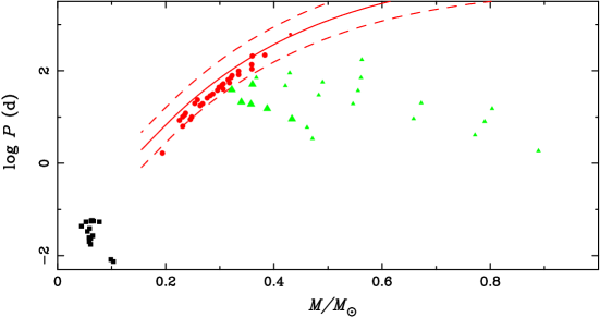
Figure 13: The final distribution of the calculated sequences in the secondary mass – orbital period plane (for sequences that avoided dynamical mass transfer). Circles and triangles indicate that the secondaries are He white dwarfs and HeCO white dwarfs, respectively. The size of the symbols indicates how much mass the neutron stars have accreted (systems with large symbols may be reasonably expected to contain millisecond pulsars). The low-mass, ultracompact systems ($M_{2}<0.15\,M_{\odot}$, $P_{\rm orb}<0.1\,$d) are plotted when the systems pass through the orbital-period minimum. The solid and dashed curves give the average and the range of the white-dwarf mass – orbital-period relation for wide binary radio pulsars (from Rappaport et al. 1995).

4 End Products

4.1 Pulsars with He, HeCO White Dwarfs

In Figure 13 we show the final distribution of the calculated systems in the secondary mass – orbital period plane (for sequences that avoided dynamical instability). Here the size of the symbols indicates how much mass a neutron star has accreted. In systems with large symbols, the neutron star has accreted at least 0.2$\,M_{\odot}$ (for our accretion prescription) and may be reasonably expected to appear as a millisecond pulsar. A circle indicates that the secondary ends its evolution as a He white dwarf. Note that the He white dwarfs form a sequence that quite closely follows the relation between white-dwarf mass and orbital period for wide binary radio pulsars as calculated by Rappaport at al. (1995; solid and dashed curves). The new sequence may be somewhat steeper at low masses (also see Ergma 1996; Tauris & Savonije 1999) and lies systematically below the average sequence of Rappaport et al. (1995). The latter can be easily understood since, when the secondaries become detached from their Roche lobes, they have already evolved somewhat away from a Hayashi track and are hotter (and hence smaller) than a giant of the same core mass (see Fig. 4), an effect that could not be easily included without detailed binary evolution calculations. This suggests that one should rescale the average relation of Rappaport et al. (1995) by a factor $\sim 0.65$.

In systems with triangle symbols, the secondaries ignite helium in the core and generally burn helium in a hot OB subdwarf phase (after mass transfer has been completed). Note that the lowest mass of a helium star for which helium can be ignited is $\sim 0.3\mbox{$\,M_{\odot}$}$, the minimum mass for helium ignition in non-degenerate cores (see, e.g., Kippenhahn & Weigert 1990). While the more massive helium stars convert most of their mass into carbon and oxygen (typically having a helium-rich envelope of at most a few per cent), the lower-mass helium stars only burn helium completely in the core and end their evolution with large helium envelopes (this was found first in calculations by Iben & Tutukov [1985] and more recently by Han et al. [2000]). It is not clear at the present time whether the fact that these low-mass HeCO white dwarfs have large CO cores has detectable, observational consequences. The most interesting aspect of the systems with HeCO white dwarfs is, of course, that most of them lie well below the white-dwarf – orbital period relation without having experienced a common-envelope phase Figure 14: Hydrogen shell flashes for a 0.199$\,M_{\odot}$ helium white dwarf originating from a secondary with an initial mass of 1.4$\,M_{\odot}$: H-R diagram (panel a); evolution of luminosity and radius as a function of time since the beginning of the initial mass-transfer phase for all flashes (panels b and d) and for just the third flash (panel c and e) with arbitrary time offset.

(also see Podsiadlowski & Rappaport 2000; Tauris et al. 2000).

Finally, it is worth noting that most of the He white dwarfs with masses $<0.4\,M_{\odot}$ and even some of the more massive HeCO white dwarfs experience several dramatic hydrogen shell flashes (typically 2 to 4) before settling on the white-dwarf cooling sequence. These flashes have been extensively discussed in the literature (e.g., Kippenhahn, Thomas, & Weigert 1968; Iben & Tutukov 1986). More recently, Sarna, Ergma, & Gerškevitš-Antipova (2000) published a detailed study of hydrogen shell flashes for low-mass He white dwarfs and their implications for the calculations of cooling ages in companions of binary millisecond pulsars.

During these flashes, the luminosity typically rises by a factor of 1000 and the radius increases by a factor of 10 or more on timescales of a few decades. Indeed, during these flashes the secondaries tend to fill their Roche lobes again, leading to several short mass-transfer phases with mass-transfer rates that are often much higher than the rates achieved in earlier phases (typically with $\dot{M}\sim\mbox{several}\times 10^{-6}\mbox{$\,M_{\odot}\,$yr${}^{-1}$}$). In Figure 14 we present an example of a He white dwarf of 0.199$\,M_{\odot}$ which experiences 3 such flashes (the secondary originally had a mass of 1.4$\,M_{\odot}$ and filled its Roche lobe near the end of the main sequence).

4.2 Ultracompact X-ray Binaries

As Figures 2a and 13 show, systems with initial orbital periods below the bifurcation period ($\sim 18\,$hr) become ultracompact binaries with minimum orbital periods in the range of 11 –$\,83\,$min. The shortest period is similar to the $11\,$min period in the X-ray binary 4U 1820-30 in the globular cluster NGC 6624 (Stella et al. 1987). Unlike the two better-known models for the formation of this system, this evolutionary channel involves neither a direct collision (Verbunt 1987) nor a common-envelope phase (Bailyn & Grindlay 1987; Rasio, Pfahl, & Rappaport 2000) and therefore constitutes an attractive alternative scenario for 4U 1820-30. This alternative evolutionary path for the origin of 4U1820-30 was originally suggested by Tutukov et al. (1987). Fedorova & Ergma (1989) made the first detailed case study of this scenario and showed that, if mass transfer starts near or just after the point of central hydrogen exhaustion, orbital periods as short as 8 min could be attained and that a system like 4U 1820-30 can pass through an orbital of 11 min twice, while approaching the period minimum and after having passed through it. In related studies, Nelson, Rappaport & Joss (1986) and Pylyser & Savonije (1988) found minimum periods as short as 34 and 38 min, respectively. These authors were not specifically trying to explain 4U 1820-30 but their Galactic counterparts 4U 1626-67 and 4U 1915-05 with orbital periods of 41 min (Middleditch et al. 1981; Chakrabarty 1998) and 50 min (Chou, Grindlay, & Bloser 2001), respectively.

Figure 15: Formation of ultracompact LMXBs. From top to bottom: the minimum orbital period, the mass of the secondary, the mass-transfer rate, and the surface hydrogen abundance (all at the minimum period) versus initial orbital period. All calculations start with a $1.4\,M_{\odot}$ neutron star and a $1\,M_{\odot}$ secondary. The vertical dashed line indicates the initial orbital period above which systems become wider rather than more compact (i.e., the bifurcation period). The dots indicate the results of the calculated sequences. The dashed curves in the top panel indicate the range of minimum periods if mass transfer is assumed to be either fully conservative (upper curve) or fully non-conservative (lower curve).

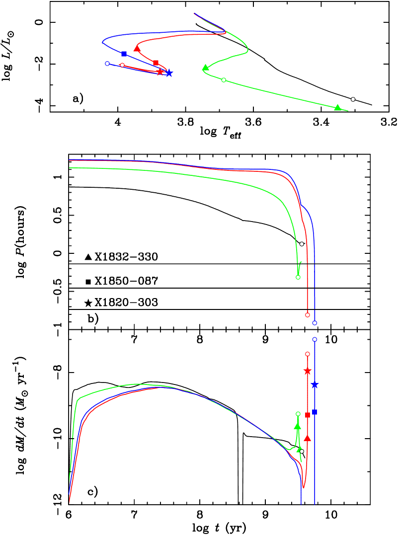
Figure 16: Selected binary sequences illustrating the formation of ultracompact LMXBs: sequence (a; black), sequence (b; green), sequence (c; red), sequence (d; blue). The individual panels show the evolutionary tracks in the H-R diagram (top), and the evolution of orbital period (middle) and mass-transfer rate (bottom) as a function of time since the beginning of mass transfer. The open circles show where the systems in the individual sequences reach their period minimums. Other symbols indicate when the systems pass through the periods of the three ultracompact LMXBs in globular clusters presently known (triangles: X1832-330; squares: X1850-087, stars: X1830-303).

Figure 17: Contact period as a function of relative capture distance for X-ray binaries that formed as a result of tidal capture. The contact period defines the initial orbital period at which mass transfer commences. The relative capture distance gives the ratio of the initial periastron distance to the radius of the star (with $M_{2}=1\mbox{$\,M_{\odot}$}$ and $Z=0.01$) captured by a neutron star (with $M_{1}=1.4\mbox{$\,M_{\odot}$}$). Different curves show the contact period for different radii (i.e., evolutionary stages) of the captured star at the epoch of capture. It is assumed that the systems are brought into contact by the combined effects of magnetic braking and evolution of the secondary.

To determine the shortest orbital period that can be attained through this channel, we performed a separate series of binary calculations for a $1\,M_{\odot}$ secondary with parameters appropriate for 4U 1820-30 in the metal-rich globular cluster NGC 6624 (i.e., with Z=0.01, Y=0.27). Our results confirm the earlier results of Fedorova & Ergma (1989) that, if the secondaries start mass transfer near the end of core hydrogen burning (or, in fact, just beyond), the secondaries transform themselves into degenerate helium stars and that orbital periods as short as $\sim 5\,$min can be attained without the spiral-in of the neutron star inside a common envelope. The top panel in Figure 15 shows the relation between initial orbital period and the minimum period, while the other panels give the secondary mass, $M_{2}$, mass-transfer rate, $\dot{M}$, and surface hydrogen abundance, $X_{\rm s}$, at the minimum period. There is a fairly large range of initial orbital periods ($13\,$–$\,17.7\,$hr) which leads to ultra-compact LMXBs with a minimum orbital period of less than $30\,$min. The drop in $P_{\rm min}$ at $13\,$hr occurs for a model where the secondary has just exhausted hydrogen in the center at the beginning of mass transfer. The shortest minimum period is attained for systems just below the bifurcation period (in this case $\sim 18\,$hr). The mass-transfer rate at the minimum period increases significantly as the minimum period decreases, simply because the time scale for gravitational radiation, which drives the evolution at this stage, becomes so short.

Figure 16 shows the details of four representative sequences: sequence (a; black) has an initially unevolved secondary, in sequence (b; green) the secondary has just completed hydrogen burning in the center, while in sequences (c; red) and (d; blue) the secondaries have pure helium cores of 0.024$\,M_{\odot}$ and 0.028$\,M_{\odot}$, respectively, at the beginning of mass transfer. Open circles show when the sequences reach the period minimum, and other symbols indicate when they pass through the periods of the three known ultracompact X-ray binaries in globular clusters (see Table 1). The shortest minimum periods are obtained for systems that exhaust all of the hydrogen left in their surface layers just near the point where they become degenerate and hence manage to transform themselves into essentially pure helium white dwarfs. In the phase where the hydrogen shell is being extinguished, the luminosity of the secondary briefly increases in the sequences with the shortest minimum periods (top panel), before the secondaries descend on the cooling sequence for He white dwarfs. In sequence (d; blue), the secondary becomes detached at an orbital period of 4.3 hr. Gravitational radiation then causes the system to shrink, and the secondary starts to fills its Roche lobe again at an orbital period of 35 min. Note also that after the minimum period, $\dot{M}$ generally drops dramatically.

In Table 1 we list all X-ray binaries in globular clusters with known orbital periods. Strikingly, three of the six systems have ultra-short periods. In this table, we also list the timescales for the orbital period changes for the three compact systems based on the sequences shown in Figure 16 as well as on a simple model where the secondary is a fully degenerate He white dwarf and the system is driven by gravitational radiation alone (labelled ‘GR’). The 11 min system (4U 1820-30 = X1820-303) is particularly interesting since its orbital period is observed to be decreasing rather than increasing (Tan et al. 1991), as would be expected for a fully degenerate secondary. While it had been argued that this apparent orbital period decrease could be caused by gravitational acceleration within the globular cluster (Tan et al. 1991), van der Klis et al. (1993) subsequently concluded that, using a more realistic mass model for the globular cluster NGC 6624, it was unlikely that the negative $\dot{P}$ could be fully explained by cluster acceleration. On the other hand, as Table 1 shows, the theoretical $P/\dot{P}$ in sequence (c; red) is in excellent agreement with the observed value, and the value in sequence (d; blue) is in reasonable agreement (Fedorova & Ergma [1989] obtained similar values). This provides additional support for this evolutionary channel for these ultracompact globular-cluster systems. One potentially testable prediction is that some of these systems still contain hydrogen in their envelopes (up to 40 % by mass in the sequences shown). After the period minimum, the secondaries in sequences (c; red) and (d; blue) become pure He white dwarfs, and their evolution is identical to that of systems with He white dwarfs, driven by gravitational radiation alone.

Since the value of the bifurcation period is sensitive to the adopted magnetic-braking law, the range of initial orbital periods which leads to ultracompact systems will also depend on it. To examine this dependence, we carried out two additional series of calculations where we increased and decreased the efficiency of magnetic braking by a factor of 5 with respect to our standard model, respectively. As expected, the bifurcation period increased to $\sim 20\,$hr for the more efficient magnetic-braking law and decreased to $\sim 15\,$hr for the less efficient one. In both cases, we obtained systems with minimum periods as short as 9 and 16 min, respectively (note, however, that this exploration was not as comprehensive as for the standard case).

It is quite remarkable that one of our binary sequences (sequence c; red), with an initial orbital period around $17\,$hr, appears to be a suitable sequence to explain all six LMXBs in globular clusters whose orbital periods are presently known, from the system with the longest period (AC211/X2127+119 in M15; $P_{\rm orb}=17.1\,$hr; Ilovaisky et al. 1993) to the 11-min binary. Furthermore, systems with an initial period in the range of $13\,$–$\,18\,$hr are quite naturally produced as a result of the tidal capture of a neutron star by a main-sequence star (Fabian, Pringle, & Rees 1975; Di  Stefano & Rappaport 1992) and are not the generally expected outcome of a 3- or 4-body exchange interaction (see, e.g., Rasio et al. 2000).

To illustrate this, we calculated the orbital period at which mass transfer commences, the contact period, for systems that form as a result of the tidal capture of a 1$\,M_{\odot}$ normal star by a 1.4$\,M_{\odot}$ neutron star. Figure 17 shows the contact period as a function of the relative capture distance (i.e., the ratio of initial periastron distance to the radius of the star) for different radii (i.e., evolutionary stages on the main sequence) of the secondary at the epoch of capture. In these calculations we assumed that the systems formed by tidal capture circularized quickly (on a timescale short compared to the magnetic-braking timescale and the evolutionary timescale of the secondary) and that the system was brought into contact by the combined effects of magnetic braking (causing the orbit to shrink) and the evolution of the secondary.

It has been estimated that for the tidal capture of a main-sequence star by a neutron star, the initial periastron distance has to be $\lesssim 3$ stellar radii (Fabian et al. 1975; Press & Teukolsky 1977; McMillan, McDermott, & Taam 1987). It also has to be larger than $\sim 1.5$ stellar radii, so that in the circularized system (which has a separation twice the initial periastron distance) the secondary underfills its Roche lobe. As Figure 17 shows, this range of initial capture distances produces systems which start mass transfer between 9 and 21 hr, depending on the radius of the secondary at the time of capture. The range of radii chosen corresponds to the change in radius of a 1$\,M_{\odot}$ star on the main sequence (i.e., as it evolves from the zero-age main sequence to the terminal-age main sequence). Since all stars on the main sequence have roughly equal probability for a dynamical encounter with a neutron star, this predicts a fairly uniform distribution of contact periods in this range. In fact, stars with a larger radius are somewhat more likely to be captured since the capture cross section increases linearly with radius (Fabian et al. 1975; Di  Stefano & Rappaport 1992). This suggests that at least half of the X-ray binaries formed by tidal capture may start mass transfer with orbital periods in the range of 13 to 18 hr, the range which produces ultracompact systems. This may explain the surprisingly large fraction of ultracompact systems (3 out of 6 systems with known orbital periods) in globular clusters.

One well-recognized problem with the tidal-capture scenario for the formation of LMXBs in globular clusters is the fact that the total energy that needs to be tidally dissipated during the capture and subsequent circularization process is of order the binding energy of the secondary. Since all of this energy is deposited in the secondary, it may lead to its destruction either by dynamical effects (Rasio & Shapiro 1991) or due to the thermally driven expansion of the secondary that is tidally heated (McMillan et al. 1987; Ray, Kembhavi, & Antia 1987; Podsiadlowski 1996). As a consequence, the initial capture distance for which a 1$\,M_{\odot}$ star can be captured and survive the process may be much more limited than the range used above. Indeed, this is the reason why it has been popular in recent years to dismiss this formation channel altogether. However, we would like to emphasize (1) that the details of the tidal capture process, in particular the response of the secondary to tidal heating (see Podsiadlowski 1996), are still rather uncertain; (2) that, as shown here, tidal capture naturally produces the range of orbital periods actually observed in globular-cluster LMXBs; and (3) that alternative scenarios, 3- or 4-body interactions, do not generally lead to systems in the observed range. This suggests to us that it is not only premature to rule out tidal capture as a formation scenario for LMXBs, but that the LMXBs in globular clusters with well-determined orbital periods actually provide observational evidence in its favor. An unbiased re-examination of the whole process is therefore clearly warranted.

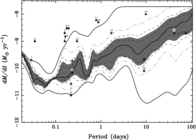
Figure 18: Cumulative (smoothed) probability distribution for the mass-accretion rate onto the neutron-star primary as a function of orbital period for the 100 binary calculations (with equal weighting for all sequences). The thick, solid central curve gives the median mass-accretion rate; the pairs of curves moving progressively outwards from the median curve include 20, 40, 60, 80, and 98 per cent of the distribution, respectively. The shaded region contains 50 per cent of all systems around the median. The symbols indicate the mass-transfer rates of selected observed X-ray binaries (triangles: Z sources; squares: atoll sources; stars: X-ray pulsars; circles: systems with accretion-disk coronae [lower limits]). The individual systems are (in ascending order of orbital period, as given in parentheses): (1) 1626-67 (0.69 hr), (2) 1916-053 (0.83 hr), (3) 1636-536 (3.8 hr), (4) 0748-676 (3.82 hr), (5) 1254-690 (3.93 hr), (6) GX9+9 (4.2 hr), (7) 1735-555 (4.65 hr), (8) 2129+470 (5.24 hr), (9) 1822-37 (5.57 hr), (10) 1658-29 (7.11 hr), (11) Sco X-1 (18.9 hr), (12), 1624-590 (21 hr), (13) Her X-1 (40.8 hr), (14) 0921-630 (216 hr), (15) Cyg X-2 (236 hr), (16) GX1+4 ($>1000\,$hr) (taken from the catalogs by van Paradijs 1995 and Christian & Swank 1997).

5 Application to the Population of X-Ray Binaries

In the previous sections we have presented the results of our 100 binary evolution models for LMXBs and IMXBs which cover a systematic grid of binary parameters at the onset of mass transfer. We have shown specifically that a number of these binary sequences pass through states which would closely resemble many of the well known and individually studied LMXBs and IMXBs. This includes X-ray binaries with long and short orbital periods, very low- to moderate-mass secondaries, a wide range of X-ray luminosities, and systems in and out of globular clusters. All but a few of our 100 binary evolution sequences started with donor stars of mass $>1M_{\odot}$, and the majority had donors $>2M_{\odot}$. One of the more striking results of these calculations is that most of the evolution time these systems spend as an X-ray binary occurs after the mass of the donor star has been reduced to $\lesssim 1M_{\odot}$ (see Fig. 2a). Thus, a large fraction of the systems which we commonly refer to as “LMXBs” may actually have started their lives as “IMXBs.” This has important implications for both (i) the retention of neutron stars in binaries at the time of the supernova explosion which gives birth to the neutron star (i.e., it is easier to keep the neutron star bound with a 2 or 3 $M_{\odot}$ companion than with a truly low-mass companion), and (ii) the evolutionary state of the companion stars in LMXBs that we observe today (i.e., they are probably not nearly as unevolved as was previously assumed).

One observational consequence is that many of these systems should be hydrogen deficient and helium enriched, and that the surface composition of many secondaries should show evidence for CNO processing (i.e., be enhanced in N and depleted in C and O). Our calculations predict that at a particular orbital period ($\gtrsim 80\,$min), the surface hydrogen abundance can vary typically between $\sim 1/3$ of the solar value and solar (at shorter orbital periods, all systems should be hydrogen-deficient). While the hydrogen (or helium) abundance can usually not be measured directly, an increased helium abundance affects the behavior of accretion, e.g., by increasing the Eddington accretion rate. This could provide some indirect evidence for helium enrichment in some of these systems.

While it is, of course, rather gratifying to be able to “explain” possible evolutionary paths leading to some of the best known X-ray binaries, there remain several outstanding issues: (1) how unique are the evolutionary paths we have found; (2) are types of systems suggested by other reasonably long-lived phases of our binary evolutions represented in the observed binary X-ray source population; and (3) is our complete ensemble of binary evolution models consistent with the overall population of observed LMXBs and IMXBs?

In order to properly investigate these questions one needs to carry out a full binary population synthesis (BPS) study, starting from primordial binaries and utilizing a library of binary evolution models of the type we have generated. Such a BPS study is beyond the scope of the present paper, but has been initiated (Pfahl et al. 2001). One objective of a BPS study will be to produce probability distributions, at the current epoch, for finding LMXBs and IMXBs with various values of $M$, $\dot{M}$, $P_{\rm orb}$, as well as in different evolutionary states, locations in the Galaxy, space velocities, and so forth. Such a study will involve weighting each of the binary evolutions in our library by the probability that each of the initial binary parameters would be realized in nature. For the present study we utilize our evolution tracks to produce a simplified estimate of the likelihood of finding LMXBs and IMXBs in various locations in the $\dot{M}-P_{\rm orb}$ plane. The choice of these two parameters – $\dot{M}$ and $P_{\rm orb}$ – is motivated by the fact that these are the easiest to determine for LMXBs. In fact, observationally, very few LMXBs and IMXBs (HZ Her/Her X-1, Cyg X-2) have well determined constituent masses or have much known about the state of the donor star. On the other hand, if an estimate of the distance is known, then $\dot{M}$ can be inferred from the X-ray luminosity (at least in the case of conservative mass transfer), and the orbital period can be inferred from X-ray or optical photometry, rather than requiring Doppler measurements of either the companion or the neutron star.

To relate our binary models to the Galactic population of LMXBs and IMXBs on a statistical basis, we have constructed a plot which estimates the probability of finding an LMXB or IMXB in a particular region of the $\dot{M}-P_{\rm orb}$ plane. We do not attempt to weight each of the binary evolution runs (in the library). We do, however, take into account the amount of time spent in a particular part of the evolution, as each of our model binaries traverses the $\dot{M}-P_{\rm orb}$ plane. We make the implicit assumption of a steady-state production of LMXBs and IMXBs which then proceed through their entire evolution, well within the lifetime of the Galaxy. This, of course, will become less valid for systems with evolutionary phases comparable to the age of the Galaxy. To construct our probability distribution in the $\dot{M}-P_{\rm orb}$ plane, we proceeded as follows. First, we divided up the $\dot{M}-P_{\rm orb}$ plane into a finely spaced, discrete, two-dimensional array. Each of the 100 binary evolution tracks was then placed into this array, weighted by the evolution time spent in each element of the array. The probability of finding an LMXB/IMXB in any particular array element is then proportional to the combined evolution time of all the tracks passing through that array element. However, since there are only 100 evolution tracks, the entire $\dot{M}-P_{\rm orb}$ plane is not completely sampled (for an analogous sampling effect in the $M-P_{\rm orb}$ plane see Fig. 2a). In order to circumvent this problem somewhat, we computed, for each value of $P_{\rm orb}$, a cumulative probability distribution in $\dot{M}$. We then utilized these to compute contours of constant probability which are plotted in Figure 18. The central heavy curve is the median value of $\dot{M}$, while the contours on either side are in increments of $10\%$ in probability, except for the top and bottom curves which represent $1\%$ and $99\%$ of the systems. The shaded region represents $50\%$ of all systems around the median.

As one can see from a perusal of Figure 18, there should theoretically be a general positive correlation between orbital period (for $P_{\rm orb}\gtrsim 1$ hr) and $\dot{M}$, with the value of $\dot{M}$ a few hundred times larger at periods of $\sim$100 days as compared with 1 hr. At a given $P_{\rm orb}$, typically half of the systems are contained within a range of about a factor of $\sim 6$ in $\dot{M}$, centered on the median value. The next step is to compare the model results shown in Figure 18 with the positions of known LMXBs and IMXBs in this diagram. We excluded all obviously transient LMXBs and IMXBs since, in most cases, it is unclear how to estimate the long-term average X-ray luminosity. We then selected 16 LMXBs and IMXBs (i) whose orbital periods are known, (ii) whose X-ray luminosities do not vary wildly, and (iii) where a distance to the source could be estimated. These are shown overplotted on Figure 18; they include 2 “Z sources” (triangles), 8 “atoll sources”(squares), 3 X-ray pulsars (stars), and 3 “accretion disk corona sources” (circles). (For references see, e.g., van Paradijs 1995; Christian & Swank 1997.) For the latter group of sources, the observed X-ray flux is thought to be severely affected by an accretion disk corona, and therefore the inferred value of $\dot{M}$ is shown only as a lower limit. We used a simple factor of $10^{-8}M_{\odot}\,{\rm yr}^{-1}\equiv 10^{38}$ erg s^-1 in converting X-ray luminosity to mass-accretion rate.

The first obvious fact in comparing the theoretical probability distribution to the locations of known LMXBs and IMXBs in the $\dot{M}-P_{\rm orb}$ plane (Fig. 18) is that only a relative handful lie plausibly in or near the shaded region. In fact, 10 of the 16 sources lie at or outside the $1\%$ upper and lower probability contours. The largest discrepancies come from luminous LMXBs with shorter orbital periods (i.e., $\lesssim$ 1 day). There are several important caveats to note before viewing the comparison made in Figure 18 as being grossly discrepant. First, as mentioned above, the evolution tracks that went into the production of the probability contours in Figure 18 are not weighted by the relative probabilities of achieving their initial binary configurations in nature. Second, no transient X-ray sources have been included in the figure. Many of these sources probably have mean values of $\dot{M}$ of $\lesssim 3\times 10^{-10}M_{\odot}\,{\rm yr}^{-1}$ (and possibly even higher for the larger values of $P_{\rm orb}$; van Paradijs 1996; King, Kolb, & Sienkiewicz 1997) which cover a substantial portion of the shaded (high probability) region. Third, there are serious observational selection effects to consider, in that it is generally true that the most luminous X-ray sources are studied in detail, yielding higher probabilities of optical identifications which, in turn, can lead to orbital period determinations. At least the first two of these shortcomings of Figure 18 will be addressed in our binary population synthesis study (Pfahl et al. 2001).

One potentially very important effect that has not been included in our binary calculations is the effect of X-ray irradiation on the secondary which could significantly alter the evolution of these systems and increase the mass-accretion rate by either driving a strong wind from the secondary (Ruderman et al. 1989) or by causing significant expansion of the secondary (Podsiadlowski 1991; Harpaz & Rappaport 1991). While these irradiation effects are still poorly understood, even a relatively moderate irradiation-driven expansion of the secondary may cause mass-transfer cycles (Hameury et al. 1993) characterized by relatively short phases of enhanced mass transfer and long detached phases. During the X-ray phases these systems would appear to be much more luminous than without the inclusion of X-ray irradiation effects. We also plan to examine this possibility in our BPS study.

6 Application to Binary Millisecond Pulsars

There are currently about 1400 radio pulsars known (Taylor, Manchester, & Lyne 1993; V. Kaspi 2001, private communication). Of these, $\sim 100$ have at least one of the following properties (V. Kaspi 2001, private communication): (i) a very short pulse period ($\sim 77$ with $P\lesssim 12\,$ms); (ii) a relatively weak magnetic field ($\sim 46$ with $B\lesssim 10^{10}\,$G); (iii) membership in a binary system ($\sim 66$); and/or (iv) location in a globular cluster ($\sim 45$). These systems are widely believed to be “recycled” pulsars, i.e., NSs whose magnetic field has decayed away and which have been spun up to high rotation rates by the accretion of matter from a companion star (see, e.g., Bhattacharya & van den Heuvel 1991). In the Galactic plane, there are several distinct classes of binary radio pulsars. One major class involves systems with low-mass companions ($0.10\,$–$\,0.4\,M_{\odot}$) and nearly circular orbits. These range in $P_{\rm orb}$ from a fraction of a day to 1000 days. There is a dearth of these pulsars in the period range of 12 and 68 days. The masses of most of the companions to these pulsars are known only approximately from the measured mass functions. Based on the scenario for their formation, which involves stable mass transfer from a low-mass giant, there is a theoretically predicted relation between the orbital period of these systems and the mass of the remnant companion white dwarf (see, e.g., Rappaport et al. 1995). In fact, the locus of points in Figure 12 tracing the maximum value of $P_{\rm orb}$ at any given white dwarf mass matches the theoretical relation rather closely (see also § 4.1). Most of the model systems helping to define this relation, however, have orbital periods between $\sim$12 and 120 days – at least the first half of which fall in the period “gap” found observationally. There is also another cluster of model systems with $P_{\rm orb}$ between $\sim$11 and 85 minutes; these are of shorter periods than any of the binary pulsars discovered thus far in the Galactic disk. Again we note the caveat discussed in § 5 that our library of binary models has not been weighted according to the probability of achieving their initial binary parameters at the onset of mass transfer, e.g., in the context of a full binary population synthesis calculation.

Another class of binary radio pulsars are the ones with substantially more massive white dwarf companions which distinctly do not fit the scenario described above (with a low-mass giant donor) and do not lie in the $P_{\rm orb}\,$–$\,M_{\rm wd}$ plane near the associated theoretical relationship. These systems also have nearly circular orbits and $P_{\rm orb}$ in the range of $\sim 1\,$– 10 days. It has been proposed for some time now that these systems result from donor stars which are more massive than the neutron star, thereby leading to unstable mass transfer and a common envelope phase (see, e.g., Taam & van den Heuvel 1986). Our models with donors that are initially of intermediate mass naturally lead to this type of system without a common envelope phase (see also § 4 and Tauris et al. 2000). Such model systems are found in abundance in Figure 13 (triangles situated well below and to the right of the theoretical curve).

Yet another class of binary radio pulsars are systems that contain planetary mass companions (i.e., $M\lesssim 0.02M_{\odot}$) which are in the process of being ablated by the radiation from the pulsar (e.g., 1957+20; Fruchter, Stinebring, & Taylor 1988). In this regard, we note that in our binary evolution calculations, the mass transfer is allowed to continue until either the donor star becomes detached from its Roche lobe or its non-degenerate envelope has been completely stripped. Of course, as the neutron star accretes matter from the companion it will be spun up by accretion torques – the maximum spin period being determined by a combination of, $\dot{M}$, the total mass accreted, and the strength of the neutron star’s magnetic field. For weak surface magnetic fields (i.e., $\lesssim 10^{9}\,$G), the accretion-induced spin period is given approximately by $P=3.5\times(\Delta M/0.01M_{\odot})^{-1/2}$ ms, where $\Delta M$ is the accreted mass. For higher magnetic fields, the minimum accretion induced rotation period scales as $1.9B_{9}^{6/7}$ ms, for an Eddington-limited luminosity, where $B_{9}$ is the surface dipole field strength in units of $10^{9}\,$G (see, e.g., Bhattacharya & van den Heuvel 1991). Thus, at some point in the evolution, prior to the exhaustion of the donor’s envelope, a spun-up neutron star may turn on as a radio pulsar. This could have two important consequences for the subsequent evolution of the binary. First, the pulsar radiation (in the form of both electromagnetic waves and a relativistic wind) may exert sufficient pressure on the incoming accretion flow that all further accretion is halted. Second, the pulsar radiation may ablate material from the donor star, and in some cases possibly evaporate it altogether (see, e.g., Ruderman, Shaham, & Tavani 1989; van den Heuvel & van Paradijs 1988, Bhattacharya & van den Heuvel 1991). In the present binary evolution calculations, we do not take either a possible pulsar turnon into account or the subsequent effects of the pulsar radiation on the donor star. In our BPS study we will attempt to use simplified prescriptions to handle both of these processes, i.e., pulsar turnon and ablation of the donor, although there are obviously still many uncertainties concerning both of these.

The final class of binary pulsars we comment on consists of a pair of neutron stars. While these systems are important for exploring binary evolution, acting as laboratories for general relativity, and yielding potentially detectable gravity wave signals when they merge, our study does not shed any new light on their formation. This results from the fact that our highest mass donor stars are $7~{}M_{\odot}$ which is too low to form a second neutron star.

Many of the same classes of binary radio pulsars that are found in the plane have also been discovered in globular clusters. In particular, there are 22 radio pulsars known in 47 Tuc (Camilo et al. 2000), 8 in M15 (Anderson 1992), and 2 each in M5, M13, Ter 5, and NGC 6624. At least 10 of the radio pulsars in 47 Tuc are in binary systems with periods ranging from 1.5 hr to 2 days. This abundance of recycled pulsars in globular clusters is widely attributed to the dense stellar environment which can lead to 2-, 3-, and 4-body stellar encounters at interestingly high rates. Thus, through a combination of processes such as 2-body tidal capture (e.g., Fabian, Pringle, & Rees 1975; Di Stefano & Rappaport 1992) and exchange interactions where a field neutron star replaces a normal star in a binary, numerous neutron star binaries should be formed (see, e.g., Rasio, Pfahl, & Rappaport 2000; Rappaport et al. 2001).

We have already discussed in § 4.2 how the globular-cluster X-ray sources fit our evolution scenarios. However, we need to check if the binary millisecond pulsars also fit naturally into the same evolutionary scenarios. In 47 Tuc, there is a group (“A”) of five pulsars which have masses of $0.02-0.03~{}M_{\odot}$ and periods of 1.5 – 5.5 hr, while a second group (“B”) has masses approximately 10 times higher and periods of 0.1 – 2 d. The evolutionary scenarios for producing the ultracompact X-ray binaries discussed in §4.2 may also provide a possible path to the formation of binary radio pulsars of the type found in the 47 Tuc group A pulsars. In the process of evolving to very short periods (11–83 min)., these mass transfer binaries will naturally pass through orbital periods of 1.5–5 hr. However, at these periods the donor masses are substantially larger than the typical values of $\sim 0.025M_{\odot}$ found for the companions in the group A systems. On the other hand, if at some point in the binary evolution, the neutron star has been spun up to msec periods, pulsar radiation may turn on and both shut off further mass transfer and ablate the donor star until it has been reduced to planetary mass. It is also true that after the minimum period is reached in the ultracompact systems (see §4.2), the orbit will, in principle, expand back into the range of about an hour or so within a Hubble time. In order for such systems to return all the way back to periods of 1.5–5 hours, some other effect, such as sustained tidal heating, would be required (as is also invoked for the case of the post-common envelope scenario proposed by Rasio et al. 2000). A characteristic of our “ultracompact” evolutionary scenario is that the correct initial orbital periods between $\sim 13-18$ hr arise naturally from tidal capture in globular clusters. By contrast, the common envelope scenario proposed by Rasio et al. (2000) follows more naturally from the wider orbits left by 3-body encounters.

The orbital period range of $\sim 0.1-2$ days for the group B pulsars is traversed in many of our binary evolutions (see, e.g., Fig. 2a). However, in all but 2 cases, the masses of the donor stars in this period range are much higher than the group B pulsar companions. In addition, the donor stars at this phase of the evolution are still quite H-rich and would therefore not resemble the inferred He white dwarf companions of these pulsars. Again, it is possible that these evolutions are interrupted by the turn-on of a strong radio pulsar at just the right values of $P_{\rm orb}$ to match the group B systems. At present, we do not have a good explanation for how this would happen, nor do we know the reason for the existence of two rather distinct groups of msec pulsars.

A long-standing problem in our understanding of millisecond pulsars, known as the birthrate problem, is that, in the standard model of LMXBs, the birthrate of LMXBs appears to be a factor of 10 to 100 lower than the birthrate of millisecond pulsars, which are believed to be their direct descendants. This problem exists for millisecond pulsars both in the Galactic disk (Kulkarni & Narayan 1988; Johnston & Bailes 1991) and in globular clusters ( Fruchter & Goss 1990; Kulkarni, Narayan, & Romani 1990). This discrepancy may be the result of an overestimate of the LMXB lifetime, typically taken to be $\sim 5\times 10^{9}\,$yr in these estimates. If a large fraction of X-ray binaries are IMXBs, one might expect that the time these systems spend as X-ray emitters could be significantly reduced, which would then alleviate the problem. However, our calculations show that even IMXBs spend most most of their X-ray active lifetime as low-mass systems and that consequently the duration of the X-ray active lifetime is generally not much lower than for true LMXBs (see the column $\Delta t_{\dot{M}}$ in Table A1). Thus the inclusion of IMXBs does not immediately solve the birthrate problem. This problem may also be related to the problem of the low median X-ray luminosities found in our calculations (as discussed in § 5) and may have a similar resolution: if irradiation-driven mass-transfer cycles operate for low-mass systems (see § 5), these would not only increase the mass-transfer rates during the X-ray active portion of the cycles but also reduce the duration of the X-ray active lifetime of these systems by a proportionate amount. This could provide a simultaneous solution to both of these problems, the X-ray luminosity and the birthrate problem.

As we have shown, our binary evolution models pertain directly to the binary radio pulsars found in both the Galactic plane and in globular clusters. However, before we can draw definitive conclusions about the relative and absolute populations of the different classes of these objects, in both the plane and in clusters, we must await the results of our binary population synthesis study (Pfahl et al. 2001).

7 Summary and Outlook

As this study has shown, the evolution of low- and intermediate-mass X-ray binaries is much more complex than previously believed, and the standard model for these systems where mass transfer is driven only by magnetic braking, gravitational radiation, and occasionally nuclear evolution is the exception rather than the rule. Our evolutionary sequences show an enormous variety of evolutionary channels which may explain the large diversity in observed systems. Indeed many of the best-studied systems in the Galactic disk (e.g., Her X-1, Cyg X-2, Sco X-1, GRO J1744-28, 4U 1626-67 and 4U 1915-05) as well as all globular clusters sources with known orbital periods can be identified with particular sequences in our library of models. This demonstrates the importance of these results for our understanding of X-ray binaries and millisecond pulsars, believed to be their descendants.

However, our results also show that there are a number of problems still remaining, in particular the low median X-ray luminosities as compared to the luminosity of well observed systems, the orbital-period distribution of millisecond pulsars, and the millisecond pulsar birthrate problem. To shed more light on the significance of these discrepancies, we have initiated a systemic binary population synthesis study (Pfahl et al. 2001) where we implement this library of models in a population synthesis code. This will not only allow us to quantify these discrepancies more precisely, but also to examine possible solutions (e.g., irradiation-driven cycles, pulsar turnon, pulsar evaporation, etc.) and should ultimately help us to improve our understanding of the evolution X-ray binaries and the formation of millisecond pulsars.

References

- (1)
- (2) Alexander, D. R., & Ferguson, J. W. 1994, ApJ, 437, 879
- (3)
- (4) Anderson, S. B. 1992, Ph.D. Thesis, California Institute of Technology
- (5)
- (6) Bailyn, C. D., & Grindlay, J. E. 1987, ApJ, 316, L25
- (7)
- (8) Baraffe, I., Chabrier, G., Allard, F. & Hauschildt, & P. H. 1998, A&A, 337, 403
- (9)
- (10) Bhattacharya, D., & van den Heuvel, E. P. J. 1991, Phys. Rep., 203, 1
- (11)
- (12) Blundell, K. M., Mioduszewski, A. J., Muxlow, T. W. B., Podsiadlowski, Ph., Rupen, M. P. 2001, ApJ, submitted
- (13)
- (14) Braun, H. 1997, Ph.D. Thesis (LMU, Munich)
- (15)
- (16) Camilo, F., Lorimer, D. R., Freire, P., Lyne, A. G., & Manchester, R. N. 2000, ApJ, 535, 975
- (17)
- (18) Casares, J., Charles, P., & Kuulkers, E. 1998, ApJ, 493, L39
- (19)
- (20) Chakrabarty, D. 1998, ApJ, 492, 342
- (21)
- (22) Chou, Y., Grindlay, J. E., & Bloser, P. F. 2001, ApJ, 549, 1135
- (23)
- (24) Davies, M. B., & Hansen, B. M. S. 1998, MNRAS, 301, 15
- (25)
- (26) Deutsch, E. W., Margon, B., & Anderson, S. F. 2000, ApJ, 530, L21
- (27)
- (28) Di Stefano, R., Nelson, L. A., Lee, W., Wood, T. H., Rappaport, S. 1997, in Thermonuclear Supernovae, NATO ASI Series, ed. P. Ruiz-Lapuente, R. Canal, & J. Isern (Dordrecht: Kluwer), 147
- (29)
- (30) Di Stefano, R., & Rappaport, S. 1992, ApJ, 396, 587
- (31)
- (32) Eggleton, P. P. 1983, ApJ, 268, 368
- (33)
- (34) Eggleton, P. P., Faulkner, J., & Flannery, B. P. 1973, A&A, 23, 325
- (35)
- (36) Ergma, E. 1996, A&A, 315, L17
- (37)
- (38) Ergma, E., & Sarna, M. J. 1996 MNRAS, 280, 1000
- (39)
- (40) Fabian, A. C., Pringle, J. E., Rees, M. J. 1975, MNRAS, 172, 15
- (41)
- (42) Faulkner, 1971, ApJ, 170, 99
- (43)
- (44) Fedorova, A. V., & Ergma, E. V. 1989, Ap&SS, 151, 125
- (45)
- (46) Finger, M. H., Koh, D. T., Nelson, R. W., Prince, T. A., Vaughan, B. A., & Wilson, R. B. 1996, Nat, 381, 291
- (47)
- (48) Fruchter, A. S., & Goss, W. M. 1990, ApJ, 365, 63
- (49)
- (50) Fruchter, A. S., Stinebring, D. R., & Taylor, J. H. 1988, Nat, 333, 237
- (51)
- (52) Hameury, J. M., King, A. R., Lasota, J. P., & Raison, F. 1993, A&A, 277, 81
- (53)
- (54) Han, Z., Tout, C. A., & Eggleton, P. P. 2000, MNRAS, 319, 215
- (55)
- (56) Harpaz, A., & Rappaport, S. 1991, ApJ, 383, 739
- (57)
- (58) Hjellming, M. S., & Webbink, R. F. 1987, ApJ, 318, 794
- (59)
- (60) Homer, L., Charles, P. A., Naylor, T., van Paradijs, J., Auriere, M., & Koch-Miramond, L. 1996, MNRAS, 282, L37
- (61)
- (62) Howell, S. B., Nelson, L. A., & Rappaport, S. 2001, ApJ, 550, 898
- (63)
- (64) Iben, I., Jr., & Tutukov, A. V. 1985, ApJS, 58, 661
- (65)
- (66) Iben, I., Jr., & Tutukov, A. V. 1986, ApJ, 311, 742
- (67)
- (68) Ilovaisky, S. A. et al. 1993, A&A, 270, 139
- (69)
- (70) in’t Zand, J. J. M. et al. 2000, A&A, 355, 145
- (71)
- (72) Johnston, S., & Bailes, M. 1991, MNRAS, 252, 277
- (73)
- (74) Joss, P. C., & Rappaport, S, 1984, ARA&A, 22, 537
- (75)
- (76) King, A. R., & Begelman, M. C. 1999, ApJ, 519, L169
- (77)
- (78) King, A. R., Kolb, U., & Sienkiewicz, E. 1997, ApJ, 488, 89
- (79)
- (80) King, A. R., Schenker, K., Kolb, U., & Davies, M. B. 2001, MNRAS, 321, 327
- (81)
- (82) King, A. R., & Ritter, H. 1999, MNRAS, 309, 253
- (83)
- (84) Kippenhahn, R., Thomas, H.-C., & Weigert, A. 1968, Z. Astrophys., 68, 256
- (85)
- (86) Kippenhahn, R., & Weigert, A. 1990, Stellar Structure and Evolution (Berlin: Springer)
- (87)
- (88) Kippenhahn, R., Weigert, A., & Hofmeister, E. 1967, in Methods in Computational Physics, Vol. 7, ed. B. Alder, S. Fernbach, & M. Rothenberg (New York: Academic), 129
- (89)
- (90) Kolb, U., & Baraffe, I. 1999, MNRAS, 309, 1034
- (91)
- (92) Kolb, U., Davies, M. B., King, A., & Ritter, H. 2000, MNRAS, 317, 438
- (93)
- (94) Kulkarni, S. R., & Narayan, R. 1988, ApJ, 335, 755
- (95)
- (96) Kulkarni, S, R., Narayan, R., & Romani, R. W. 1990, ApJ, 356, 174.
- (97)
- (98) Landau, L. D., Lifshitz, E. M. 1959, The Classical Theory of Fields (Pergamon Press: Oxford)
- (99)
- (100) Langer, N., Deutschmann, A., Wellstein, S., & Höflich, P. 2000, A&A, 361, 1046
- (101)
- (102) Lewin, W. H. G., van Paradijs, J., & van den Heuvel, E. P. J. (eds.) 1995, X-Ray Binaries (Cambridge, Cambridge Univ. Press)
- (103)
- (104) McMillan, S. L. W., McDermott, P. N., & Taam, R. E. 1987, ApJ, 318, 261
- (105)
- (106) Middleditch, J., Mason, K. O., Nelson, J. E., White, N. E. 1981, ApJ, 244, 1001
- (107)
- (108) Nelson, L. A., Rappaport, S. A., & Joss, P. C. 1986, ApJ, 304, 231
- (109)
- (110) Orosz, J. A., & Kuulkers, E. 1999, MNRAS, 305, 132
- (111)
- (112) Paczyński, B. 1970, in IAU Colloq. 6, Mass Loss and Evolution in Close Binaries, ed. K. Gyldenkerne & R. M. West (Copenhagen: Copenhagen University Publications), 139
- (113)
- (114) Paczyński, B. 1976, in Structure and Evolution in Close Binary Systems, ed. P. P. Eggleton, S. Mitton, & J. Whelan (Dordrecht: Reidel), 75
- (115)
- (116) Paczyński, B., & Sienkiewicz, R. 1972, Acta Astron., 22, 73
- (117)
- (118) Paczyński, B., & Sienkiewicz, R. 1981, ApJ, 248, L27
- (119)
- (120) Pennington, R. P. 1986, Ph.D. Thesis (Cambridge University), unpublished
- (121)
- (122) Pfahl, E. D., Podsiadlowski, Ph., & Rappaport, S. 2001, in preparation
- (123)
- (124) Podsiadlowski, Ph. 1991, Nat, 350, 136
- (125)
- (126) Podsiadlowski, Ph. 1996, MNRAS, 279, 1104
- (127)
- (128) Podsiadlowski, Ph., & Rappaport, S. 2000, ApJ, 529, 946
- (129)
- (130) Pols, O. R., Tout, C. A., Schröder, K.-P., Eggleton, P. P., & Manners, J. 1997, MNRAS, 289, 869
- (131)
- (132) Press, W. H., & Teukolsky, S. A. 1977, ApJ, 213, 183
- (133)
- (134) Press, W. H., Teukolsky, S. A., Vetterling, W. T., Flannery, B. P. 1992, Numerical Recipes in Fortran: the Art of Scientific Computing (Cambridge: Cambridge University Pres), Chapter 9.3
- (135)
- (136) Pylyser, E. H. P., & Savonije, G., J. 1988, A&A, 191, 57
- (137)
- (138) Pylyser, E. H. P., & Savonije, G., J. 1989, A&A, 208, 52
- (139)
- (140) Rappaport, S., Di Stefano, R., & Smith, M. 1994, ApJ, 426, 692
- (141)
- (142) Rappaport, S., & Joss, P. C. 1997, ApJ, 486, 435
- (143)
- (144) Rappaport, S. Joss, P. C., & Webbink, R. F. 1982, ApJ, 254, 616
- (145)
- (146) Rappaport, S., Pfahl, E., Rasio, F., & Podsiadlowski, Ph. 2001, in Evolution of Binary and Multiple Star Systems, ASP Conf. Proc., Vol. 229, ed. Ph. Podsiadlowski, S. Rappaport, A. R. King, F. D’Antona, & L. Burderi (San Francisco, ASP), 409
- (147)
- (148) Rappaport, S., Podsiadlowski, Ph., Joss, P. C., Di Stefano, R., & Han, Z. 1995, MNRAS, 273, 731
- (149)
- (150) Rappaport, S., Verbunt, F., & Joss, P. C. 1983, ApJ, 275, 713
- (151)
- (152) Rasio, F. A., Pfahl, E. D., & Rappaport, S. 2000, ApJ, 532, L47
- (153)
- (154) Rasio, F. A., & Shapiro, S. L., 1991, ApJ, 377, 559
- (155)
- (156) Ray, A., Kembhavi, A. K., & Antia, H. M. 1987, A&A, 184, 164
- (157)
- (158) Ritter, H. 1988, A&A, 202, 93
- (159)
- (160) Ritter, H. 1996, in Evolutionary Processes in Binary Stars, ed. R. A. M. J. Wijers, M. B. Davies, & C. A. Tout (Dordrecht: Kluwer), 223
- (161)
- (162) Ritter, H., & Kolb, U. 1998, A&AS, 129, 83
- (163)
- (164) Rogers, F. J., Iglesias, C. A. 1992, ApJS, 79, 507
- (165)
- (166) Ruderman, M., Shaham, J., & Tavani, M. 1989, ApJ, 336, 507
- (167)
- (168) Ruderman, M., Shaham, J., Tavani, M., & Eichler, D. 1989, ApJ, 343, 292
- (169)
- (170) Sansom, A. E. Dotani, T., Asai, K., & Lehto, H. J. 1993, MNRAS, 262, 429
- (171)
- (172) Sarna, M. J., Ergma, E., & Gerškevitš-Antipova, J. 2000, MNRAS, 316, 84
- (173)
- (174) Savonije, G. J., de Kool, M., & van den Heuvel, E. P. J. 1986, A&A, 155, 51
- (175)
- (176) Sawada, E., Hachisu, I., & Matsuda, T. 1984, MNRAS, 206, 673
- (177)
- (178) Schröder, K.-P., Pols, O. R., Eggleton, P. P. 1997, MNRAS, 285, 696
- (179)
- (180) Soberman, G. E., Phinney, E. S., & van den Heuvel, E. P. J., 1997, A&A, 327, 620
- (181)
- (182) Spruit, H. C., & Ritter, H. 1983, A&A, 124, 267
- (183)
- (184) Stella, L., White, N., & Priedhorsky, W. 1987, ApJ, 315, L49
- (185)
- (186) Christian, D. J., & Swank, J. H. 1997, ApJS, 109, 177
- (187)
- (188) Taam, R. E., & van den Heuvel, E. P. J. 1986, ApJ, 302, 235.
- (189)
- (190) Tan, J., et al. 1991, ApJ, 374, 291
- (191)
- (192) Tauris, T. M., & Savonije, G. J. 1999, A&A, 350, 928
- (193)
- (194) Tauris, T. M., van den Heuvel, E. P. J., & Savonije, G. J. 2000, ApJ, 530, L93
- (195)
- (196) Taylor, J. H., Manchester, R. N., & Lyne, A. G. 1993, ApJS, 88, 529.
- (197)
- (198) Thomas, H.-C. 1967, Z. Astrophys., 67, 420
- (199)
- (200) Thorne, K. S., & Żytkow, A. N. 1977, ApJ, 212, 832
- (201)
- (202) Tutukov, A. V., Fedorova, A. V., Ergma E., & Yungelson, L. R. 1985, SvA, 11, 123
- (203)
- (204) Tutukov, A. V., Fedorova A. V., Ergma E., & Yungelson L. 1987, Sov. Astron. Lett., 13, 328
- (205)
- (206) van den Heuvel, E. P. J., & van Paradijs, J. 1988, Nat, 334, 227.
- (207)
- (208) van der Klis, M., et al. 1993, MNRAS, 260, 686
- (209)
- (210) van Paradijs, J. 1995, in X-Ray Binaries, ed. W. H. G. Lewin, J. van Paradijs, & E. P. J. van den Heuvel (Cambridge: Cambridge University Press), 536
- (211)
- (212) van Paradijs, J. 1996, ApJ, 464, L139
- (213)
- (214) Verbunt, F. 1987, ApJ, 312, 23
- (215)
- (216) Verbunt, F., & Zwaan, C. 1981, A&A, 100, L7
- (217)
- (218) Witte, M. G., & Savonije, G. J. 2001, A&A, 366, 840
- (219)