hep-ph/0107256

SNS-PH/01-10

SN1a data and the CMB of Modified Curvature at Short and Large Distances

Mar Bastero-Gil and Laura Mersini

Scuola Normale Superiore and INFN, Piazza dei Cavalieri 7,
I-56126 Pisa, Italy

The SN1a data, although inconclusive, when combined with other observations makes a strong case that our universe is presently dominated by dark energy. We investigate the possibility that large distance modifications of the curvature of the universe would perhaps offer an alternative explanation of the observation. Our calculations indicate that a universe made up of no dark energy but instead, with a modified curvature at large scales, is not scale-invariant, therefore quite likely it is ruled out by the CMB observations. The sensitivity of the CMB spectrum is checked for the whole range of mode modifications of large or short distance physics. The spectrum is robust against modifications of short-distance physics and the UV cutoff when: the initial state is the adiabatic vacuum, and the inflationary background space is de Sitter.

E-mails: bastero@cibs.sns.it, mersini@cibs.sns.it

1 Introduction

Based on the theoretical cosmological models of inflation, the interpretation of the current astrophysical observations such as the SN1a data [1], suggest that our universe contains a large amount of dark energy [2].

However, alternative models, free of dark energy, which may fit in the allowed range of parameters suggested by observation, are not excluded. In this paper we investigate claims to a possibly different interpretation of the SN1A data, for these alternative cosmological models: a FRW universe with no dark energy but with a modified curvature at large enough distances. The hope then is that either the Friedman equation for the expansion is modified, or that the light from SN1a that reaches us, while passing through these regions of different curvature, would be deflected, thereby “appearing” to have the same effect as an accelerating universe^,.

We examine metric perturbations in this modified background geometry (traced back at the time of inflation). Metric perturbations are responsible for the generation of the large scale structure and temperature anisotropies of the CMB. The inflaton field (in 4 dimensions), through the Friedmann equation, determines the expansion rate $H$ for the curvature of the background geometry. The metric perturbations satisfy a Klein-Gordon scalar field equation, minimally coupled to gravity [4]. The scalar field has a generalized mass squared $\Omega_{n}(\eta)^{2}$ that receives the contributions of two terms: the field frequency squared and the field coupling to the background curvature term. The coupling of the field to the curvature results in a modified propagation at long wavelengths since the curvature of the universe is modified at large distances compared to the intermediate scales. Examples of modified gravity can be found in [5, 6, 7, 8]. Then, the modified propagation of wavelengths of the same scale as the background curvature deviation scale can be attributed to a nonlinear dispersed frequency of the field at those wavelengths, for as long as the generalized mass squared, $\Omega_{n}(\eta)^{2}$ in the field equation, remains the same. This equivalence noticed in [9] is very useful for calculating the effects of modified large distance curvature in observations.

Our model consists of a (2-parameter) family of nonlinear dispersion relations for the generalized frequency of the field, that take account of the modification of the curvature at large distances. The family of dispersion functions is nearly linear for most of the range $k<M_{P}$, except a nonlinear deviation centered around some low value of momenta $k_{0}$. It is this deviation bump that reflects the modifications of the generalized frequency of the field at low momenta $k_{0}$ due to the modification of the curvature at large distances $k^{-1}_{0}$. The dispersion function introduced in Sect. 2, although nonlinear in the transplanckian regime, it is nevertheless a smooth function there, asymptotically approaching a constant value at time-infinity, thus having a well defined initial vacuum state [10]. The analytical calculation of the CMB spectrum is based on the Bogoliubov coefficient method. The details of the exact solutions for this class of dispersion functions [10] are given in the Appendix.

In Sect. 3 we check the sensitivity of CMB spectrum to the bump parameters $k_{0}$ and $B$ (scale location and amplitude) that control the deviation behavior from a linear frequency dispersion at low values of the momenta; i.e., the allowed range of curvature modifications at very large or very short distances that may agree with observation. We use CMBFAST in Sect. 3 to plot the spectrum, by replacing the standard primordial power spectrum $\delta_{H}^{0}(k)$ with that derived analytically in Sect. 2 for the model considered. We comment and summarize the results in Section 4. It is shown that the CMB spectrum is sensitive only to the choice of the initial vacuum state and the departure from linearity in the low momenta regime. However, for an adiabatic initial vacuum state, the CMB spectrum of a de Sitter expansion does not depend in the details of nonlinearity in the transplanckian regime [11, 12, 13, 9, 14, 15] .

2 The Model

The generalized Friedmann-Lemaitre-Robertson-Walker (FLRW) line-element in the presence of scalar and tensor perturbations, takes the form [16]

$$ds^{2} = a^{2}(\eta)\left\{-d\eta^{2}+\left[\delta_{ij}+h(\eta,{\bf n})Q\delta_{ij}\right.\right.$$ (1)

$$\left.\left.+h_{l}(\eta,{\bf n})\frac{Q_{ij}}{n^{2}}+h_{gw}(\eta,{\bf n})Q_{ij}\right]dx^{i}dx^{j}\right\}\,,$$

where $\eta$ is the conformal time and $a(\eta)$ the scale factor. The dimensionless quantity ${\bf n}$ is the comoving wavevector, related to the physical vector ${\bf k}$ by ${\bf k}={\bf n}/a(\eta)$. The function $(h,\,h_{l})$ and $h_{gw}$ represent the scalar and tensor perturbations respectively.

The power spectrum of the perturbations can be computed once we solve the equations in the scalar and tensor sector. The equation for the metric perturbations corresponds to a Klein-Gordon equation of a minimally coupled scalar field, $\mu_{n}$, in a time dependent background

$$\mu_{n}^{\prime\prime}+\Omega_{n}(\eta)^{2}\mu_{n}=0\,,$$ (2)

where the prime denotes derivative with respect to conformal time $\eta$, and the generalised comoving frequency is

$$\Omega_{n}(\eta)^{2}=n^{2}-\frac{a^{\prime\prime}}{a}=a^{2}k^{2}-\frac{a^{\prime\prime}}{a}\,.$$ (3)

The dynamics of the scale factor is determined by the evolution of the background inflaton field $\phi$, with potential $V(\phi)$, and the Friedmann equation. There are mechanisms that may produce different scale factors by modifying gravity at large (e.g. [5, 6, 7, 8]) or short distances ([13]).The present large distance modification scales can be traced back in time and would correspond to deviations in the primordial scale factor and spectrum. We can denote this “distance-dependent” scale-factor by ${\cal A}$. The coupling of the field to this background curvature results in a modified propagation of the field at long wavelengths. Therefore, modifications of the scale factor or curvature ($\mathcal{A}$) of the universe at large scales can be attributed to a dispersed effective frequency $(n_{eff})$, such that the generalized comoving frequency Eq. (3) remains the same, in the following manner

$$\Omega_{n}(\eta)^{2}=n^{2}-\frac{\mathcal{A}^{\prime\prime}}{\mathcal{A}}=n_{eff}^{2}-\,\frac{a^{\prime\prime}}{a}\,.$$ (4)

$n_{eff}$ denotes the dispersed comoving frequency of the field due to absorbing the modification terms to the curvature, ${\cal A}^{\prime\prime}/{\cal A}$. Therefore, the dispersion function for the generalized frequency results from the modified curvature at very large and very short distances. It deviates from linearity at small momentum $k$ and asymptotically approaches a constant value in the transplanckian regime.

The dispersion relation for the generalized comoving frequency $\Omega_{n}(\eta)$ is simply [10]: $\Omega_{n}(\eta)=a(\eta)F[n/a(\eta)]$. The 2-parameter family of dispersion functions $F[k]$ of our model (see Fig. 1) is:

$$F[k]^{2} = (k^{2}-k_{1}^{2})V_{0}(x,x_{0})+k^{2}~{}V_{1}(x-x_{0})+k_{1}^{2}\,,$$ (5)

$$V_{0}(x,x_{0}) = \frac{C}{1+e^{x}}+\frac{E~{}e^{x}}{(1+e^{x})(1+e^{(x-x_{0})})}\,,$$ (6)

$$V_{1}(x-x_{0}) = -B\frac{e^{x}}{(1+e^{(x-x_{0})})^{2}}\,,$$ (7)

where the dimensionless wavevector is $x=k/k_{C}$, $k_{C}=M_{P}$ is the cutoff scale, $k_{0}\ll k_{C}$, (i.e. $x_{0}\ll\ 1)$ is the value at which we deviate from linearity at low momentum, the deviation amplitude is controlled by the parameter $B$, and the constant parameter $k_{1}<k_{C}$ is the asymptotic value of the frequency in the transplanckian regime ($k\rightarrow\infty$). $C,E,B,x_{0}$ are dimensionless parameters.

Figure 1: Shown is one of the members of the family of dispersion relations $\Omega_{n}(\eta)^{2}$ as a function of: (a)$\Omega_{k}^{2}=a^{2}F[k]^{2}$ as a function of the physical momentum $x$; (b) conformal time $\eta$. The variable $x=k/k_{C}$ has been shifted by 1 such that the regime of linear dispersion relation corresponds to small positive values of momenta, i.e., $x\ll 1$.

As already discussed in Refs. [11, 12, 13], Eq. (2) represents particle production in a time-dependent background [18, 19]. We will follow the method of Bogoliubov transformation to calculate the spectrum. The frequency $\Omega_{n}(\eta)^{2}$ (which is the same as a ‘time-dependent mass squared‘ term) goes asymptotically to constant values at late and early times. Therefore the initial and final vacuum states are well defined. At early times the wavefunction should behave as a plane wave:

$$\mu_{n}\rightarrow_{\eta\rightarrow-\infty}\frac{1}{\sqrt{2\Omega_{n}^{in}}}e^{-i\Omega^{in}_{n}\eta}\,.$$ (8)

But at late times one has a squeezed state due to the curved background that mixes positive and negative frequencies. The evolution of the mode function $\mu_{n}$ at late times fixes the Bogoliubov coefficients $\alpha_{n}$ and $\beta_{n}$,

$$\mu_{n}\rightarrow_{\eta\rightarrow+\infty}\frac{\alpha_{n}}{\sqrt{2\Omega^{out}_{n}}}e^{-i\Omega^{out}_{n}\eta}+\frac{\beta_{n}}{\sqrt{2\Omega^{out}_{n}}}e^{+i\Omega^{out}_{n}\eta}\,.$$ (9)

with the normalization condition:

$$|\alpha_{n}|^{2}-|\beta_{n}|^{2}=1\,.$$ (10)

In the above expressions, $\Omega^{in}_{n}$ and $\Omega^{out}_{n}$ denote the asymptotic values of $\Omega_{n}(\eta)$ when $\eta\rightarrow\mp\infty$.

Details of the exact solution for Eq. (2) with the dispersed frequency given by Eqs. (5-7) are given in the Appendix. The final expression for the Bogoliubov coefficient $|\beta_{n}|^{2}$ is:

$$|\beta_{n}|^{2}=\frac{\sinh^{2}(2\pi\hat{\Omega}_{-})+\Gamma(k_{0},B)}{\sinh^{2}(2\pi\hat{\Omega}_{+})-\sinh^{2}(2\pi\hat{\Omega}_{-})}\,,$$ (11)

where $\hat{\Omega}_{i}=\Omega_{i}/n$, $\hat{\Omega}_{\pm}=(\hat{\Omega}^{out}\pm\hat{\Omega}^{in})/2$, and the deviation function $\Gamma(k_{0},B)$ that contains the departure from thermality in the spectrum is

$$\Gamma(k_{0},B)=\cosh^{2}(\frac{\pi}{2}\sqrt{4Be^{-x_{0}}-1})\,.$$ (12)

When $B=0$, for $\Omega^{in}>\Omega^{out}$, then it is clear from Eq. (11) that the spectrum of created particles is nearly thermal to high accuracy,

$$\left|\frac{\beta_{n}}{\alpha_{n}}\right|^{2}\simeq e^{-4\pi\sqrt{C}}\,.$$ (13)

The function $\Gamma(k_{0},B)$ represents the $deviation$ of the spectrum from thermal behavior due to the non-linearities at low momentum. Therefore, the amplitude of the power spectrum, $\delta_{H}(k)$, will be modified by $\Gamma(k_{0},B)$ due to the non-linear dispersion function introduced at around $x_{0}<1$.

In de Sitter space, the Bogoliubov coefficients would not depend on $k$ except their dependence in the bump parameters through the deviation function $\Gamma(k_{0},B)$. This function represents the departure from thermality in the particle creation number, $|\beta_{n}|^{2}$ and it confirms B. L. Hu idea [20] that near thermal radiance can be characterized by departure from exponential scaling. It is straightforward to derive the CMB power spectrum, $P(n)$, analytically from (the exact solution for) the Bogoliubov coefficients $\alpha_{n},\beta_{n}$ [15]

$$P(n)=\frac{n^{3}}{2\pi^{2}}|\frac{\mu_{n}}{a}|^{2}\simeq|\beta_{n}+\alpha_{n}|^{2}\,.$$ (14)

The deviation of the spectrum from scale-invariance in this class of models depends on the parameters of large-distance curvature modifications, namely: the scale of modified long wavelength modes, $k_{0}^{-1}$, and the deviation amplitude $B$.

The expression for the Bogoliubov coefficient and Eq. (13) indicate that: for a well-defined initial vacuum state, the spectrum is insensitive to the nonlinear dispersion relation in the transplanckian regime (modifications of short-distance physics). The unusual CMB spectrum plotted in the next Section with CMBFAST, demonstrates that modifications of the large scale curvature of the universe produce a tilt due to the departure from scale-invariance, and therefore conflict with the observed CMBR spectrum. In general the tilt is enhanced for modifications at superhorizon scales ($k_{0}\leq H_{0}$) because it is the low energy modes that dominate the spectrum in the Bogoliubov coefficient. Although departure from scale invariance is smaller at the last scattering horizon scale, $H_{LS}$, the range of deviation parameters is constrained by the amplitude of the first peak. The deviation introduced to the spectral index, $n_{s}$ from higher energy modes (wavelengths shorter than the last scattering horizon $k_{0}>H_{LS}$) becomes negligible because high energy modes do not contribute significantly to the spectrum. However, the shorter wavelengths would correspond to the intermediate FRW regime rather than the large distance scales, a regime which is scrutinized by direct observation.

3 CMB Spectrum

Recent Boomerang and MAXIMA-1 CMB experiments [21, 22] have, to high accuracy, constrained the cosmological parameters, derived from the family of inflationary adiabatic models, to: total energy density $\Omega_{tot}=0.90\pm 0.15$ and spectral index $n_{s}=0.99\pm 0.09$ at a 95% confidence level [23]. The current data favors a universe with dark energy density $\Omega_{\Lambda}=0.7$.

In this part, we explore the cosmological consequences of the alternative model that was given in Section 2 (Fig. 1). CMB is the most difficult test of precision cosmology that these models should pass. This model contains no dark energy, $\Omega_{\Lambda}=0$, however it describes a universe which at large distances has a modified curvature from the metric of the FRW universe at intermediate scale. In Fig.2 we show the CMB power spectra obtained for different representative values of the deviation parameters $k_{0}$ and $B$ in the dispersion function Eqs. (5-7). The conventional parameters that go in the input of CMBFAST are: $(\Omega_{tot},\Omega_{b},\Omega_{c},\Omega_{\Lambda}$), which stand for total energy density, baryonic, cold dark matter and the cosmological constant energy density respectively; and $n_{s}$ which is the scalar spectral index. We modified the power spectrum amplitude $\delta_{H}^{0}(k)$ in the POWERSFLAT subroutine of CMBFAST, in order to contain the deviation from the thermal spectrum (for the exact calculation reported in Section 2). The modified perturbation amplitude $\delta_{H}^{2}(k)$ is expressed in terms of $\delta_{H}^{0},\,k_{0},\,B$, where $\delta_{H}^{0}$ is the unmodified amplitude of the scale-invariant power spectrum, $k_{0}$ corresponds to the location-scale where the curvature is modified, and B measures the amplitude of deviation in the curvature at scale $k_{0}$.

The values of the conventional parameters were taken to be (1,0.03, 0.97,0) for all the deviation plots ($II-V$), but the deviation parameters in the 4 plots below in Fig. 2 are in respective order:

I	(solid line):	($k_{0}=0$, $B=0$, $\Omega_{\Lambda}=0.7$)
II	(long-dashed line):	($k_{0}=10^{-6}$ hMpc-1, $B=2$)
III	(dashed line):	($k_{0}=0.05$ hMpc-1, $B=2$)
IV	(dot-dashed line ):	($k_{0}=5$ hMpc-1, $B=2$)
V	(dotted line ):	($k_{0}=0.05$ hMpc-1, $B=2.5$)

All plots were normalized to COBE. Shown for comparison is also plot $I$ corresponding to the conventional CMB spectrum with $\Omega_{\Lambda}=0.7$. As it can be seen from the plots in Fig. 2, there are distinct features of the CMB spectra corresponding to the dispersion function in comparison to the standard spectrum obtained for ($\Lambda$)CDM models.

There is an overall tilt produced in the spectrum which signals departure from the scale invariance. This tilt is a function of the amplitude and scale of the modification, $k_{0},B$, introduced in Sect.2 (Eq.11), such that it increases for low values of the deviation momentum scale $k_{0}$ and large deviation amplitude $B$. Let us consider the 3 regimes into which the curvature modifications can be introduced:

(1) Modifications at superHubble scales ($k_{0}<H_{0}$). The departure from scale invariance is the strongest because the low energy modes dominate the spectrum, (II) in Fig. 2. Models predicting curvature modifications in regime (1) quite likely are ruled out due to a strongly tilted spectrum.

(2) Modifications in the distance range between the current horizon $H_{0}$ and last scattering horizon scale $H_{LS}$ ($H_{0}\leq k_{0}\leq H_{LS}$). For this range, the tilt is less pronounced then in regime (1). The main constraint comes from the tilt and it tightly limits the amplitude of deviation in the first peak. For modifications around the last scattering horizon scale, $k_{0}\approx H_{LS}$ the departure from scale invariance is vanishing, therefore the constraints are relaxed. However, even in this case the parameter B is tightly constrained to deviation by less than 10%, in order for the amplitude of the first peak $A_{1}$ to be in the allowed range of 4500-5500 $\mu K^{2}$ [21, 22]. In Fig. 2 we show the CMB spectra for these tuned values of $k_{0},\,B$; for comparison we also plotted the CMB for a value of $B=2.5$, which is outside the allowed range.

(3) Modifications at distances shorter than the last scattering horizon ($k_{0}>H_{LS}$). As we approach higher energy modes, the effect of the modification in the tilt of the spectrum is suppressed, therefore the departure from the conventional spectrum is vanishing. Nevertheless, these length scales do not correspond to large distances anymore, instead they are in the intermediate regime of FRW Universe. Thus the possibility of curvature modifications at such scales (galactic and intergalactic) is ruled out by direct observation up to very short distances (less than 1 mm). Clearly, there is no tilt or departure from the conventional CMB produced in the limit of modifications of very short distance physics, (very high momenta $k_{0}\rightarrow\infty$, i.e., transplanckian regime).

The claim of the model was to “offer an alternative explanation” to the SN1a data, namely: either the conventional Friedmann equation is modified or; the light of the SN1a passing through regions of modified curvature would get deflected, and therefore when received by us would appear as if indicating an accelerating universe. Although this alternative approach to the SN1a data might be theoretically appealing, we conclude that the CMB data tightly constrains it and makes it unlikely to bear any resemblance to reality. The method used in this work, can also be adopted to check if higher dimensional models that predict modified gravity at large scales and modified equations for the perturbations [5, 6, 7, 8] satisfy the CMB constraints.

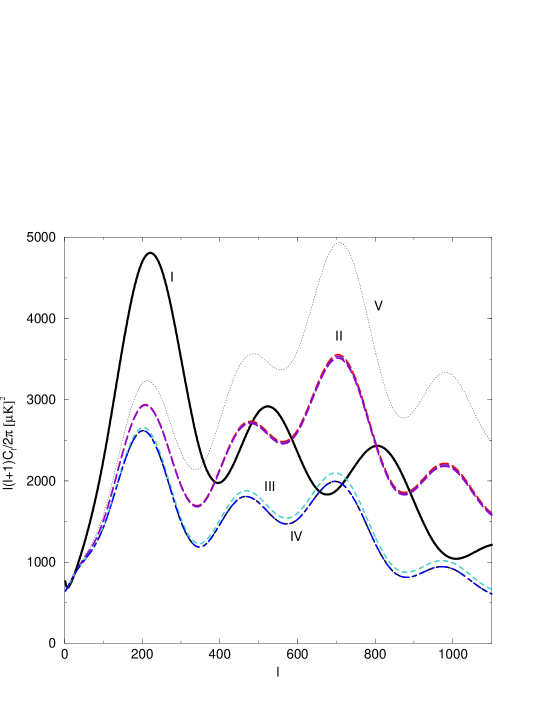
Figure 2: The CMB spectrum corresponding to our model for three different representative values of the deviation parameters $k_{0}$ and fixed deviation amplitude $B=2$, $II-IV$. Shown is also the case of a larger amplitude $B=2.5$ at scale $k_{0}\approx H_{LS}$ (V). The CMB plots were obtain using CMBFAST and they were normalised to COBE.

4 Summary

In this work we investigated claims that a modified large-distance curvature may offer an alternative explanation for the SN1a data. To check these claims, we studied the sensitivity of CMB spectrum to the whole range of modes, $0\leq k\leq\infty$, when short and large distance regimes are modified.

In [9] it was noticed that a modified curvature of the universe at large distance (when traced back at the time of inflation) gives rise to a dispersed frequency for the cosmic perturbations. The field is minimally coupled to the curvature thus its propagation feels the modifications in the background geometry. We adopted the method of Ref. [9] in order to find out the effects of curvature deviations on the current astrophysical observables.

The role of a modified curvature of the universe at large distances on the inflationary metric perturbations was analytically described by a family of dispersion relations. The modification modulates the generalized frequencies of the inflationary perturbation modes at small values of the momenta $k$ by departing from linearity around some certain small momenta $k=k_{0}$ ($k_{0}\leq M_{P}$) with a deviation amplitude $B$. The nonlinear feature of the dispersion relations, at small momenta $k_{0}$ and in the transplanckian regime, tracks the curvature deviations at large and short distances, from the conventional FRW universe of intermediate scales. One of the parameters ($k_{1}^{2}<k_{C}^{2}$), in this class of dispersion functions was constrained in order to satisfy the Starobinsky bound for negligible backreaction [14].

The analytical expression for the CMBR spectrum (Sect. 2), as well as the CMBFAST plots of this class of models, deviate from the black body scale invariant spectrum. The deviation function $\Gamma(k_{0},B)$, given in Sect. 2 and the Appendix, which measures departure from the scale-invariant spectrum (deviation from thermality in the the Bogoliubov coefficient), depends on two free parameters, the scale $k_{0}$ and the amplitude of the curvature modifications $B$. The tilt produced in the spectrum due to $\Gamma(k_{0},B)$ is present for all modification scales $k_{0}\leq M_{P}$ (these values of the physical momenta correspond to the time of inflation). The tilt is less pronounced for scale modifications corresponding to length scales less or equal to the horizon of the last scattering surface, and in this case, the main constraint comes from the modifications to the amplitude of the first acoustic peak and the fact that curvature modifications in the intermediate FRW Universe scales are under direct observation. It remains interesting to answer why the only curvature modifications that for a small range of $k_{0}$ and $B$ can reconcile with the conventional CMB spectrum are allowed only around the last scattering $H_{LS}$ scales.

The scale and amplitude of the deviations from the conventional spectrum, are severely constrained from the observed CMB spectrum to be within $10\%$ of the scale and amplitude of the first peak. Although it is counterintuitive, since large distance would correspond to low energy theories, our results indicate that any modifications in the large scale curvature of the universe, is tightly constrained from CMB data, to a very small range of deviations from the curvature of the intermediate FRW universe. Perhaps, there is a natural way that would explain such a universe with an FRW spacetime at intermediate and very large distances but with small curvature deviations around $H_{LS}$, without the need to appeal to fine-tuning. But if not, then theoretical cosmological models would have to account for the negative pressure dark energy of the universe.

The analysis of the sensitivity of the CMB spectrum for the whole range of modes in a de Sitter background space, with modifications in the short and large distance physics, reveal: the spectrum is insensitive to the details of short-distance physics and the cuttoff scale $k_{C}$ (the transplanckian regime) only for an initial adiabatic vacuum state; the scale-invariance of the spectrum and the amplitude of the first acoustic peak are very sensitive to modifications of large distance physics (low momentum modes); the spectrum is also highly sensitive to the choice of the initial conditions. In our class of dispersion models, the initial vacuum state is well-defined since the background ($\Omega_{n}(\eta)^{2}$) goes asymptotically flat at early times (Bunch-Davis vacuum [25]). The CMB spectrum for this class of models is indeed insensitive to short distance modifications, as it can be checked by taking the limit when large scale modification parameters ${k_{0},B}$ go to zero, in which case the conventional scale-invariant spectrum is recovered. Therefore all the features observed in Fig. 2, are due to large-scale curvature modifications only.

Acknowledgment: We are very grateful to S.Dodelson for his help with the CMBFAST. We want to thank A. Riotto, R. Kolb, L. Parker, A. Kempf, P. Frampton, G. Siegl, I. Kogan, for beneficial discussions and comments. We also would like to thank P. Kanti for useful discussions in the early stages of this work. We acknowledge Lloyd Knox for making CMBFAST program available.

5 Appendix

The family of dispersion functions we used in Sect. 2 to model the deviation of the curvature at large and short distances is given by:

$$F[k]^{2} = (k^{2}-k_{1}^{2})V_{0}(x,x_{0})+k^{2}~{}V_{1}(x-x_{0})+k_{1}^{2}\,,$$ (15)

$$V_{0}(x,x_{0}) = \frac{C}{1+e^{x}}+\frac{E~{}e^{x}}{(1+e^{x})(1+e^{(x-x_{0})})}\,,$$ (16)

$$V_{1}(x-x_{0}) = -B\frac{e^{x}}{(1+e^{(x-x_{0})})^{2}}\,,$$ (17)

where $x=k/k_{C}$, $x_{0}=k_{0}/k_{C}$; $k_{C}=M_{P}$ is the cutoff scale, $k_{0}\ll k_{C}$ ($x_{0}\ll 1$) is the value at which we deviate from linearity at low momentum, and the amplitude of the “bump/deviation” is controlled by $B$ (see Fig. 1). The parameter $k_{1}=n_{1}/a(\eta)$ gives the asymptotic constant value at initial time for the frequency in the limit ($k\gg k_{C}$), i.e., in the transplanckian regime. On the other hand, in order to ensure the linear behavior at very low values of the momenta, $x\ll 1$, we impose the following constraints for any value of the deviation parameters $x_{0}$ and B:

$$V_{0}(x\ll 1,x_{0}) \simeq 1\,,\;\;\;\;\;V_{0}(x\ll 1,x_{0})^{\prime\prime}\simeq 0\,,$$ (18)

$$V_{1}(x\ll 1,x_{0}) \simeq 0\,,$$ (19)

where prime denotes derivative with respect to the physical momentum $k$. The generalised comoving frequency $\Omega_{n}(\eta)$ is then given by:

$$\Omega_{n}(\eta)^{2} = a(\eta)^{2}F[n/a(\eta)]^{2}$$ (20)

$$= \!\!\!\!(n^{2}-n_{1}^{2})\left[\frac{C}{1+e^{x}}+\frac{E~{}e^{x}}{(1+e^{x})(1+e^{(x-x_{0})})}\right]-n^{2}\left[\frac{B~{}e^{x}}{(1+e^{(x-x_{0})})^{2}}\right]+n_{1}^{2}\,,$$

with $n=a(\eta)k$, $a(\eta)=-|\eta_{C}|/\eta$ during de Sitter inflation ($|\eta_{C}|=1/H(\eta_{C})$), and

$$x=\frac{k}{k_{C}}=-\frac{n}{|\eta_{C}|k_{C}}\eta\,.$$ (21)

The generalised frequency $\Omega_{n}(\eta)$ goes to constant values at $\eta\rightarrow\pm\infty$, such that:

$$\Omega_{n}(\eta) \rightarrow_{\eta\rightarrow-\infty} \Omega_{n}^{in}=n_{1}\,,$$ (22)

$$\Omega_{n}(\eta) \rightarrow_{\eta\rightarrow+\infty} \Omega_{n}^{out}=\sqrt{n_{1}^{2}+C(n^{2}-n_{1}^{2})}\,,$$ (23)

with $\Omega_{n}^{out}\simeq\sqrt{C}n$ when $n\gg n_{1}$.

Under the change of variables $\eta\rightarrow u=exp(dn\eta)$, where $d=1/(|\eta_{C}|k_{C})$, the scalar wave equation (2) for the mode $\mu_{n}$ becomes:

$$\left[\partial^{2}_{u}+\frac{1}{u}\partial_{u}+V(u)\right]\mu_{n}=0\,,$$ (24)

where:

$$V(u)=\hat{D}+\frac{\hat{C}}{u(1+u)}+\frac{\hat{E}}{u(u+1)(\gamma_{0}+u)}-\frac{\hat{B}}{u(u+\gamma_{0})^{2}}\,,$$ (25)

and,

$$\hat{C}=C[(n^{2}-n^{2}_{1})/(n~{}d)^{2}]\,,\;\;\;\hat{E}=E[(n^{2}-n^{2}_{1})/(n~{}d)^{2}]\,,$$

$$\hat{D}=(n_{1}/n~{}d)^{2}\,,$$

$$\hat{B}=B/d^{2}\,,$$

and $\gamma_{0}=exp(-k_{0}/k_{C})$. Eq. (24) is exactly solvable in terms of the Riemann generalised hypergeometric functions [26] with the constraint $\hat{E}=\hat{C}/(1-\gamma_{0})$,

$$\mu_{n}\propto P\left(\begin{array}[]{cccc}0&\infty&-\gamma_{0}&\\ a&c&b&u\\ a^{*}&c^{*}&b^{*}&\end{array}\right)\,.$$ (26)

As explained in Section 2, because of the asymptotic behavior of $\Omega_{n}(\eta)$, the initial and final vacua are well defined and the mode functions $\mu_{n}$ behave as plane waves in the asymptotic limits $\eta\rightarrow\mp\infty$. The exact solution which matches this asymptotic behavior is then given by:

$$\mu^{in}(\eta)=N^{in}(u)^{a}(u+\gamma_{0})^{b}~{}_{2}F_{1}[a+b+c,a+b+c^{*},1+a-a^{*},-\frac{u}{\gamma_{0}}]\,,$$ (27)

where $N^{in}$ is a normalization constant, and

$$a = -i\hat{\Omega}^{in}=-i\sqrt{\hat{D}}\,,$$ (28)

$$b = \frac{1}{2}\left(1+\sqrt{1-4\hat{B}e^{-x_{0}}}\right)\,,$$ (29)

$$c = -i\hat{\Omega}^{out}=-i\sqrt{\hat{D}+\hat{C}}\,.$$ (30)

At late times the solution becomes a squeezed state by mixing of positive and negative frequencies:

$$\mu^{out}_{n}(\eta)\!\!\!\!\!\! = N^{out}~{}(u)^{a}(u+\gamma_{0})^{b}\times$$

$$\!\!\!\!\!\!\left(\frac{\Gamma(1+a-a^{*})\Gamma(c^{*}-c)}{\Gamma(a+b+c^{*})\Gamma(1-a^{*}-b-c)}~{}_{2}F_{1}[a+b+c,a^{*}+b+c,1+c-c^{*},-\frac{\gamma_{0}}{u}]\right.$$

$$+ \!\!\!\!\!\!\left.\frac{\Gamma(1+a-a^{*})\Gamma(c^{*}-c)}{\Gamma(a+b+c)\Gamma(1-a^{*}-b-c^{*})}~{}_{2}F_{1}[a+b+c^{*},a^{*}+b+c^{*},1+c^{*}-c,-\frac{\gamma_{0}}{u}]\right)\,,$$

$$\mu^{out}_{n} \rightarrow_{\eta\rightarrow+\infty} \frac{\alpha_{n}}{\sqrt{2\Omega^{out}_{n}}}e^{-i\Omega^{out}_{n}\eta}+\frac{\beta_{n}}{\sqrt{2\Omega^{out}_{n}}}e^{+i\Omega^{out}_{n}\eta}\,,$$ (31)

with $|\beta_{n}|^{2}$ being the Bogoliubov coefficient equal to the particle creation number per mode $n$ and $\hat{\Omega}_{i}=\Omega_{i}/n$. Using the linear transformation properties of hypergeometric functions [26], we find that

$$\left|\frac{\beta_{n}}{\alpha_{n}}\right|^{2}=\frac{\sinh^{2}(2\pi\hat{\Omega}_{-})+\Gamma(k_{0},\hat{B})}{\sinh^{2}(2\pi\hat{\Omega}_{+})+\Gamma(k_{0},\hat{B})}\,,$$ (32)

where,

$$\hat{\Omega}_{\pm}=\frac{\hat{\Omega}^{out}\pm\hat{\Omega}^{in}}{2}\,,\;\;\;\;\hat{\Omega}^{(}i)=\frac{\Omega^{i}}{nb}\,,$$ (33)

and the deviation function $\Gamma(k_{0},\hat{B})$ is

$$\Gamma(k_{0},\hat{B})=\cosh^{2}(\frac{\pi}{2}\sqrt{4\hat{B}e^{-x_{0}}-1})\,.$$ (34)

When $B=0$ and $\Omega^{in}>\Omega^{out}$, then it is clear from Eq. (32) that the spectrum of created particles is nearly thermal to high accuracy,

$$\left|\frac{\beta_{n}}{\alpha_{n}}\right|^{2}\simeq e^{-4\pi\sqrt{C}}\,,$$ (35)

as expected in de Sitter expansion. However, when $B\neq 0$, $\gamma_{0}\neq 0$, at the mode crossing time $n=Ha(\eta)$, we can write:

$$\left|\frac{\beta_{n}}{\alpha_{n}}\right|^{2}\approx e^{-4\pi\sqrt{C}}\left[\frac{1+\frac{\Gamma(k_{0},B)}{\sinh^{2}2\pi\hat{\Omega}_{-}}}{1+\frac{\Gamma(k_{0},B)}{\sinh^{2}2\pi\hat{\Omega}_{+}}}\right]\,.$$ (36)

The expression in the squared bracket in the above equation contains the deviation from scale invariance. The deviation $\Gamma(k_{0},B)$ is larger at low values of the momentum modification scale, $x_{0}\ll 1$. On the other hand, $\Gamma(k_{0},B)$ is suppressed around large scales, $x_{0}\simeq 1$. The same results about the scale dependence of the deviation function were obtained by using CMBFAST code (Figs. 2).

References

- [1] S. Perlmuttter et al., Astrophys. J. 517, 565 (1999); A. G. Riess et al, Astron. J, 116, 1009 (1998); astro-ph/0104455.
- [2] S. Perlmutter, M. S. Turner and M. White, Phys. Rev. Lett. 83, 630 (1999); L. M. Krauss, astro-ph/0102305; J. L. Tonry, astro-ph/0105413. S. Carroll, Living Rev. Rel.4:1,2001.
- [3] P. P. Avelino, J. P. M. de Carvalho, C. J. A. P. Martins and J. C. R. E. Oliveira, astro-ph/0004227; P. P. Avelino, J. P. M. de Carvalho and C. J. A. P. Martins, astro-ph/0103075; P. P. Avelino, A. Canavezes, J. P. M. de Carvalho and C. J. A. P. Martins, astro-ph/0106245.
- [4] For a review, see for example: V. Mukhanov, H. Feldman and R. H. Brandenberger, Phys. Rep. 215, 203 (1992), and references therein.
- [5] I. I. Kogan, S. Mouslopoulos, A. Papazoglou, G. G. Ross and J. Santiago, Nucl. Phys. B584 (2000) 313; I. I. Kogan and G. G. Ross, Phys. Lett. B 485 (2000) 255; I. I. Kogan, S. Mouslopoulos, A. Papazoglou and G. G. Ross, Nucl. Phys. B595 (2001) 225; I. I. Kogan, S. Mouslopoulos and A. Papazoglou, Phys. Lett. B 503 (2001) 173.
- [6] C. Csáki, J. Erlich and T. J. Hollowood, Phys. Rev. Lett. 84 (2000) 5932; Phys. Lett. B481 (2000) 107.
- [7] R. Gregory, V. A. Rubakov and S. M. Sibiryakov, Phys. Rev. Lett. 84 (2000) 5928; hep-th/0003045.
- [8] C. Deffayet, Phys. Lett. B502 (2001)199; G. Dvali, G. Gabadadze and M. Porrati, Phys. Lett. B485 (2000) 208; C. Deffayet, G. Dvali and G. Gabadadze, astro-ph/0105068. See also: P. P. Avelino and C. J. A. P. Martins, astro-ph/0106274, for constraints on this kind of models.
- [9] L. Mersini, M. Bastero-Gil and P. Kanti, hep-ph/0101210; L. Mersini, hep-ph/0106134; M. Bastero-Gil, hep-ph/0106133.
- [10] L. Mersini, Int. J. Mod. Phys. A13, 2123 (1998).
- [11] J. Martin and R. H. Brandenberger, hep-th/0005209; R. H. Brandenberger and J. Martin, astro-ph/0005432.
- [12] J. C. Niemeyer, Phys. Rev. D63, 123502 (2001); J. C. Niemeyer and R. Parentani, astro-ph/0101451.
- [13] A. Kempf, Phys. Rev. D63, 083514 (2001); A. Kempf and J. C. Niemeyer, astro-ph/0103225; T. Jacobson, hep-th/0001085; T. Jacobson and D. Mattingly, gr-qc/0007031; hep-th/0009052; M. Visser, C. Barceló and S. Liberati, hep-th/0109033.
- [14] T. Tanaka, astro-ph/0012431; A. A. Starobinsky, astro-ph/0104043.
- [15] R. Easther, B. R. Greene, W. H. Kinney and G. Shiu, hep-th/0104102.
- [16] E. M. Lifshitz and I. M. Khalatnikov, Adv. Phys. 12, 185 (1963); L. P. Grishchuk, Phys. Rev. D50, 7154 (1994).
- [17] L. P. Grishchuk, Zh. Eksp. Teor. Fiz. 67, 825 (1974); J. Martin and D. Schwarz, Phys. Rev. D57, 3302 (1998).
- [18] L. Parker, Phys. Rev. 183, 1057 (1969); R. U. Sexl and H. K. Urbantke, Phys. Rev. 179, 1247 (1969); Y. Zel’dovich and A. Starobinsky, Zh. Sksp. Teor. Fiz. 61, 2161 (1971) [Sov. Phys. JETP 34, 1159 (1971)]; Ya. Zel’dovich, Pis’ma Zh. Eksp. Teor. Fiz. 12, 443 (1970) [Sov. Phys. JETP Lett. 12, 302 (1970)]; B. L. Hu, Phys. Rev. D9, 3263 (1974); S. W. Hawking, Nature 248, 30 (1974); Comm. Math. Phys. 43, 199 (1975); W. G. Unruh, Phys. Rev. D14, 870 (1976); B. K. Berger, Phys. Rev. D12, 368 (1975); L. Parker, Naure 261, 20 (1976); in “Asymptotic Structure of Space-Time”, eds. F. P. Esposito and L. Witten (Plenum, New York, 1977).
- [19] N. D. Birrell and P. C. W. Davies, “Quantum fields in curved space-time” (Cambridge University Press, Cambrigde, 1982).
- [20] B. L. Hu, in Proc. CAP-NSERC Summer Institute in Theoretical Physics, Vol. 2, Edmonton, Canada, 1987( World Scientific, Singapore, 1988); B. L. Hu and Y. Zhang, “Coarse-graining, scaling and inflation”, Univ. Maryland preprint 90-186 (1990); B. L. Hu, in Relativity and Gravitation: Classical and Quantum, Proc. SILARG VII, Cocoyoc, Mexico, 1990 (World Scientific, Singapore, 1991); A. Raval, B. L. Hu and D. Koks, Phys. Rev. D55, 4795 (1997).
- [21] P. de Bernardis et al., Nature 404, 955 (2000); A. Balbi et al., astro-ph/0005124; A. H. Jaffe et al., astro-ph/0007333.
- [22] A. T. Lee et al., astro-ph/0104459; C. B. Netterfield et al., astro-ph/0104460; N. W. Halverson et al., astro-ph/0104489.
- [23] A. E. Lange et al, Phys. Rev. D63, 042001 (2001); C. Pryke et al., astro-ph/0104490; R. Stompor et al., astro-ph/0105062; P. de Bernardis et al., astro-ph/0105296;
- [24] L. Pilo, R. Rattazzi and A. Zaffaroni, hep-th/0004028.
- [25] T. D. Bunch and P. C. W. Davies, Proc. Roy. Soc. Lond. A360, 117 (1978).
- [26] M. Abramowitz and A. I. Stegun (eds.), “Handbook of Mathematical Functions” (New York, Dover, 1965).