CHEMICAL EVOLUTION OF CLUSTERS OF GALAXIES

The high metallicity of the intra–cluster medium (ICM) is generally interpreted on the base of the galactic wind scenario for elliptical galaxies. In this framework, we develop a toy–model to follow the chemical evolution of the ICM, formulated in analogy to chemical models for individual galaxies. Just as the ingredients for usual models are (a) the stellar yields, amount of metals newly synthesized and re-ejected by stars; (b) the Star Formation Rate and (c) the stellar Initial Mass Function (IMF), our model for clusters involves: (a’) “galactic yields” derived from galactic wind models of ellipticals; (b’) a parametric Galactic Formation Rate; (c’) a Press-Schechter-like Galactic Initial Mass Function.
The model is used to test the response of the predicted metal content and abundance evolution of the ICM to varying input galactic models. The resulting luminosity function of cluster galaxies is also calculated, in order to constrain model parameters.

Introduction

The popular galactic wind (GW) scenario, introduced by Larson (1974) to account for the photometric properties of elliptical galaxies, predicted as a side effect the pollution of the intra–cluster medium (ICM) with the chemical elements produced and expelled by individual galaxies (Larson & Dinerstein 1975). Metals in the hot ICM were in fact detected soon afterwards (Mitchell et al. 1976, Serlemitsos et al. 1977).

The amount of metals present in the ICM, as reported by Renzini (1997), is currently estimated as:

$$\frac{M_{ICM}^{Fe}}{M_{*}^{Fe}}=\frac{Z_{ICM}^{Fe}\,M_{ICM}}{Z_{*}^{Fe}\,M_{*}}=1.65\,h^{-3/2}$$

with obvious meaning of the symbols. Iron is generally used as tracer of the overall metallicity, being the best measured element in the hot ICM. With $h\sim 0.65$, three times more metals seem to be spread in the ICM than locked into the stellar component of the individual galaxies.

The source of such a large amount of metals in the ICM could be galactic (as in the original prediction by Larson) or reside in Population III pre-galactic objects (White & Rees 1978). The distinct correlation between the iron mass in the ICM and the luminosity of elliptical and S0 galaxies,

$$M_{ICM}^{Fe}\propto L_{V}^{E+S0}$$

demonstrated by Arnaud et al. (1992), seems to favour galaxies as the sites of production of the metals in the ICM.

Accepting that the metals in the ICM originated in the E and S0 galaxies of the cluster, two mechanisms exist to extract the newly sinthesized elements from the individual galaxies: the above mentioned GW and ram pressure stripping. Arguments have been given by Renzini (1997) favouring the GW scenario, mostly based on the observation that the “iron mass–to–luminosity ratio” (IMLR) is roughly constant independently of cluster richness and temperature, while the ram pressure mechanism should be more efficient, extracting more metals for a given stellar content, in richer clusters.

Though the role of ram pressure stripping is still debated (e.g. Mori & Burkert 2000), from here on we will limit to the GW scenario for the pollution of the ICM, bearing in mind that the addition of other mechanisms (metal production in pre-galactic objects and/or ram pressure stripping) would allow to inject even more metals into the ICM, further favouring the enrichment.

1 The gas and metal content of the ICM

In this section we briefly summarize previous literature and current understanding of the gas and metal content in the ICM, from the point of view of theoretical models of galactic chemical evolution with GWs.

1.1 The metal content of the ICM

Various early studies investigated whether “standard” chemical models for galaxies can explain the amount of metals detected in the ICM (Vigroux 1977, Himmes & Biermann 1980, De Young 1978); by “standard” we mean a chemical model with the same physical ingredients (mainly, stellar Initial Mass Funstion and yields) suited to reproduce the Solar Neighbourhood. Amidst these early studies, we mention in particular the one by Matteucci & Vettolani (1988), as the first attempt to link directly the metallicity of the ICM with the properties of the corresponding galaxy population. To this aim, the authors developed a modelling technique that has been widely adopted afterwards. Basing on a grid of models of elliptical galaxies with GW, they assigned to any given galaxy of final stellar mass $M_{*}$, or equivalently of final present–day luminosity $L_{*}$, the corresponding masses of gas and iron ejected in the GW ($M^{ej}_{gas}$, $M^{ej}_{Fe}$). Integrating these quantities over the observed luminosity function (LF), they calculated the total masses of gas and iron globally ejected by the galactic population in the cluster. Their main conclusions were:
(1) the iron content of the ICM can be reproduced with a standard Salpeter Initial Mass Function (IMF) in the individual galaxies;
(2) the global amount of gas ejected as GW is much smaller than the observed mass of the ICM, hence the ICM must be mostly primordial gas which was never involved in galaxy formation.

This early successful reproduction of $M_{Fe}^{ICM}$ turned out afterwards to be favoured by the low gravitational potential wells of model galaxies, calculated only on the base of their luminous, baryonic component. Once the potential well of the much heavier dark matter halo is included, the ejecta of SN Ia hardly escape the galaxy and the metal pollution of the ICM by GWs is much reduced (David et al. 1991, Matteucci & Gibson 1995). In this case, standard chemical models fail to reproduce the metal content of the ICM. Some non–standard scenarios were thus invoked to solve the riddle, such as:

• a more top–heavy IMF than the Salpeter one, with logarithmic slope $x\sim 1.0$ rather than the standard value $x=1.35$ (Matteucci & Gibson 1995, Gibson & Matteucci 1997ab, Loewenstein & Mushotzky 1996);

• a bimodal IMF with an early generation of massive stars heavily polluting the ICM, followed by a more normal star formation phase producing the stars we see today (Arnaud et al. 1992, Elbaz et al. 1995).

These models, where SN II from massive stars play the main role in the metal pollution of the ICM, were further supported by the enhanced abundances of $\alpha$–elements with respect to iron detected with ASCA (e.g. Mushotzky et al. 1996; but see nowadays the revised, low oxygen abundances measured with XMM, Mushotzky, this conference).

In brief, a wealth of work in literature suggests that some non–standard scenario (or IMF) must be invoked to account for the metals in the ICM. We recall that a non–standard IMF has been suggested for elliptical galaxies also on the base of other, independent arguments:

• a top–heavy IMF ($x\sim 1.0$) is better suited to reproduce the photometric properties of ellipticals (Arimoto & Yoshii 1987);

• sistematic variations of the IMF in ellipticals of increasing mass might explain the increase of the $M/L$ ratio with galactic luminosity, that is the so–called “tilt of the Fundamental Plane” (Larson 1986, Renzini & Ciotti 1993, Zepf & Silk 1996).

1.2 The amount of intra-cluster gas

Just as in the early work by Matteucci & Vettolani (1988), most authors conclude that GWs cannot account for the huge amount of gas present in the ICM (2–5 times the mass in galaxies, Arnaud et al. 1992). The ICM must then consist, for a 50 to 90%, of primordial gas.

Trentham (1994), on the base of the steep slope of the LF at the low luminosity end observed in clusters, suggested that all the intra–cluster gas could have originated in dwarf galaxies, since these are numerous in clusters and they are expected to eject a large fraction of their initial mass as GW, due to their shallow potential wells. This suggestion was discarded by Nath & Chiba (1995) and by Gibson & Matteucci (1997a), who calculated detailed models of dwarf galaxies and related GW ejection to show that galaxies cannot be the only source for the whole intra–cluster gas, even in the case of the steepest observed LF (hence the largest contribution from dwarfs).

2 A non–standard IMF

As mentioned in § 1.1, many authors have suggested that some non-standard IMF must be invoked to explain the amount of metals in the ICM. What physical reason may justify a different IMF in different situations?

Larson (1998) suggested the following functional form of the IMF:

$$\frac{dN}{d\log{M}}\propto M^{-x}exp\left(-\frac{M_{s}}{M}\right)$$

where $M_{s}$ is a typical mass scale related to the Jeans mass. In brief, this IMF is a (Salpeter–like) power law down to a typical peak mass

$$M_{p}\sim\frac{M_{s}}{x}$$

below which there is an exponential cut-off. The peak mass varies with the temperature and density conditions of the parent gas as

$$M_{p}\propto T^{2}\,\rho^{-\frac{1}{2}}$$

as expected from Jeans’ law. In warmer and/or less dense gas, therefore, the typical peak mass $M_{p}$ increases; namely, relatively more massive stars are formed while less mass remains locked into ever-living, very low–mass stars (lower locked-up fraction, e.g. Tinsley 1980).

A similar behaviour is predicted by the theoretical IMF by Padoan et al. (1997, hereinafter PNJ), which features a peak mass

$$M_{p}=0.2M_{\odot}\left(\frac{T}{10K}\right)^{2}\left(\frac{n}{1000K}\right)^{-\frac{1}{2}}\left(\frac{\Sigma_{g}}{2.5~{}km~{}sec^{-1}}\right)^{-1}$$

Although the physical derivation of the PNJ IMF has been sometimes questioned (e.g. Scalo et al. 1998), one can still adopt it in galactic models as a tentative recipe, yielding the behaviour naïvely expected for the typical Jeans mass; see Chiosi (2000) for further discussion.

2.1 Galactic models with the PNJ IMF

Chiosi et al. (1998) developed chemo–thermodynamical models following the thermodynamical evolution of the gas in an elliptical galaxy, and the corresponding variations in the IMF according to the PNJ recipe. The characteristics and behaviour of these models as a function of galactic mass and redshift of formation are discussed in full details in Chiosi et al. (1998) and Chiosi (2000). Here, we briefly underline the qualitative trends with respect to (a) mass and (b) redshift of formation.

(a)

At increasing galactic mass, the average density of the object $\rho$ decreases and the typical peak mass $M_{p}$ increases, yielding a lower locked-up fraction.

(b)

At increasing redshift $z_{for}$ of formation, the temperature of the object increases, since it can never fall below the corresponding temperature of the cosmic microwave background, $T\geq T_{CMB}(z_{for})$, which increases with redshift; hence, the peak mass $M_{p}$ is higher and the locked–up fraction is lower.

We remark here that the above mentioned trends are by no means drastic: the peak mass $M_{p}$ never exceeds 1 $M_{\odot}$, and the “high $M_{p}$” phase is limited to the early galactic ages; after the initial stage, in fact, the system reaches a sort of thermodynamical balance, with the peak mass and the IMF settling on quite standard values. The overall picture loosely resembles the bimodal behaviour suggested by Elbaz et al. (1995), with an early phase dominated by massive stars followed by a more normal star formation phase producing the low–mass stars we see today. However, in our models the IMF naturally and smoothly varies in time following a physical prescription.

Though not long-lasting, the variations in the early phases are enough to differentiate the resulting galactic models, making them successful at reproducing many features of observed ellipticals, such as (Chiosi et al. 1998):

• the tilt of the Fundamental Plane (§ 1.1)

• the analogous of the “G–dwarf” problem, or the lack of a large population of low metallicity stars, detected in the spectral energy distribution of ellipticals (Bressan et al. 1994, Worthey et al. 1996);

• the high fraction of white dwarfs (Bica et al. 1996);

• both the colour–magnitude relation and the trends in $\alpha$–enhancement with mass at the same time, thereby overcoming the well-known dichotomy between the “classic” and “inverse” GW scenario (Matteucci 1992, 1994, 1997).

This last point is worth commenting further, as the GW modelling influences directly the predictions concerning the ICM. GW models of elliptical galaxies with a constant IMF (whether Salpeter or more top–heavy) face the following puzzle. The colour–magnitude relation suggests that GWs occur later in more massive ellipticals than in smaller ones, so that star formation and chemical enrichment proceed longer and the stellar population reaches redder colours in more luminous objects. On the other hand, metallicity indices, if interpreted as abundance indicators, suggest that the [Mg/Fe] ratio increases with galactic mass; this requires GWs to occur earlier in more massive galaxies, where only SN II should contribute to the chemical enrichment to make the resulting abundance ratios in stars $\alpha$–enhanced.

This dichotomy between the so–called “classic” and “inverse” GW scenario, hampers predictions of the metal pollution of the ICM, since two competing sets of GW models are to be considered. It is therefore quite appealing, when we address the chemical enrichment of the ICM, that the variable IMF scenario described above can reproduce both observational constraints, with a unique set of models.

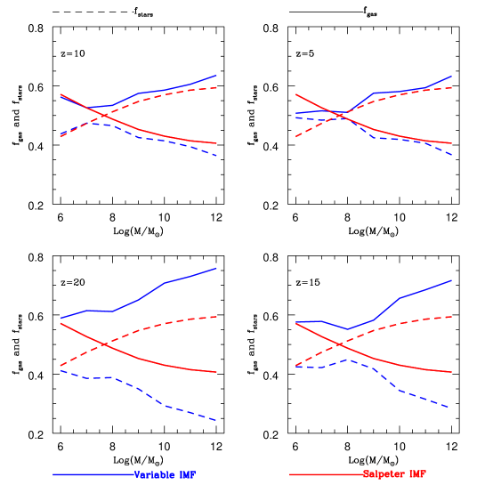
Figure 1: Mass fraction of ejected gas (solid lines) and complementary fraction locked into stars (dashed lines) as a function of the initial (baryonic) galactic mass. The four panels correspond to models with different redshifts of formation, as indicated. Red lines: galaxy models with Salpeter IMF; blue lines: models with variable PNJ IMF.

2.2 Galactic ejecta: PNJ vs. Salpeter IMF

Chiosi (2000) first analyzed what are the predictions about the metal pollution of the ICM when galaxy models with the PNJ IMF are adopted. To this purpose, he calculated multi–zone chemical models of ellipticals with the PNJ IMF.

The adoption of radial multi–zone models, rather than simple one–zone models, has in fact noticeable consequences on the predicted enrichment of the ICM, as first underlined by Martinelli et al. (2000). When the radial structure of an elliptical galaxy is considered, with the corresponding gradients in density, colours etc., it turns out that the GW tends to develop not instantly over the whole galaxy, but earlier in the outskirts (where the potential well is shallower) and later in the central parts. This means that star formation and chemical enrichment proceed longer in the centre than in the outer regions (Tantalo et al. 1998, Martinelli et al. 1998), and the GW ejected from different galactic regions is metal enriched to different degrees.

The models calculated by Chiosi (2000) account for these effects by dividing the galaxy into three zones: a central sphere where star formation and metal production is most efficient and lasts longer; an intermediate shell where the GW sets in earlier and the metal production proceeds to a lesser extent, and an outer corona where the gas is expelled almost immediately, with virtually no star formation and chemical processing. This behaviour is the combined result of the shallower potential well when moving outward in the galaxy (as in standard models with a constant IMF) and of the varying $M_{p}$ in the PNJ IMF when moving to outer, less dense regions; see Chiosi (2000) for a detailed discussion.

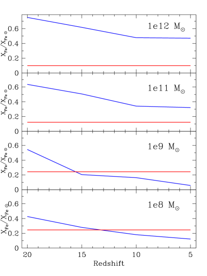
Figure 2: Metallicity (iron abundance) of the gas ejected as GW from galaxies of given initial (baryonic) mass, indicated in the individual plots, and as a function of their redshift of formation. Blue lines: galactic models with the PNJ IMF; red-lines: comparative results for models with the Salpeter IMF, which are redshift independent.

For the sake of comparison, analogous models with the standard Salpeter IMF were also calculated. For a better understanding of the results concerning the chemical evolution of the ICM, let’s first inspect the predicted GW ejecta of the galactic models when the variable IMF or the Salpeter IMF are adopted in turn.

In Fig. 1 we compare the mass fraction of gas ejected in the GW, and the complementary mass fraction locked into stars, for galactic models with the variable PNJ IMF and for models with the Salpeter IMF (blue and red lines, respectively). Mass fractions refer to the total initial baryonic mass of the (proto)galaxy. The amount of ejected gas is larger in the case of the PNJ IMF, since less mass is locked into low-mass stars, thanks to the high $M_{p}$ in the early galactic phases. The difference with the Salpeter case gets sharper for larger (proto)galactic masses, and for higher redshifts of formation. (Notice that models with the Salpeter IMF bear no dependence on the redshift of formation, as there are no temperature effects on the IMF in this case).

It is worth underlining here the following “inverse” behaviour of the models with the PNJ IMF with respect to what is generally expected from models with a constant IMF. According to the general consensus, larger galaxies store a larger fraction of their mass into stars and eject a lower fraction of gas in the GW, while smaller galaxies are more efficient in wind ejection, due to their shallower potential wells. This behaviour is in fact found in the Salpeter galactic models of Fig. 1. The models with the PNJ IMF, on the other hand, show quite the opposite behaviour: larger galaxies eject a larger fraction of their initial mass in the wind and lock a lower fraction into stars, due to the higher peak mass that characterizes them in the early phases. This effect overwhelms their deeper potential wells, and the trend becomes stronger and stronger with the redshift of formation.

Fig. 2 shows the iron abundances in the gas ejected as GW, again comparing the Salpeter IMF (red lines) and the PNJ IMF case (blue lines). In most cases, the galactic ejecta in the PNJ models are more metal–rich than in the Salpeter case, up to a factor of 5 or more in the case of the more massive galaxies, and for high redshifts of formation. In the PNJ models, in fact, more gas in the galaxy gets recycled through massive stars, effective metal contributors, and less gets locked into low–mass stars, before the GW occurs.

From the trends described above, we expect that models of ellipticals with the PNJ IMF predict, for the ICM, a more efficient metal pollution and a higher fraction of the gas originating from GWs, with respect to “standard” models. The first results in this respect are discussed in Chiosi (2000).

3 The chemical evolution of the ICM: a toy model

As mentioned in § 1.1, the most popular way to calculate the expected properties of the ICM of a cluster, on the base of its population of elliptical galaxies, is to make use of a grid of galactic models and integrate their GW ejecta over the observed LF, a method first developed by Matteucci & Vettolani (1988). In this approach, all the ellipticals in the cluster are assumed to be coeval, of an age around 13-15 Gyrs.

If we are to adopt here galactic models with the PNJ IMF, however, results are expected to be very sensitive to the exact epoch (redshift) of formation of the individual galaxies. The usual integration over the present–day LF is not a viable method in our scenario: the present-day luminosity of a galaxy no longer provides enough information to identify it (in terms of its initial protogalactic mass) since the final properites of a galactic model depend not only on its initial mass, but also on its exact formation redshift. Hence, we need to follow in detail the epoch of formation of the individual galaxies in the cluster, and evolve the overall system down to the present–day, using then the LF as a constraint a posteriori. This approach also allows, in principle, a more self–consistent description of the chemical evolution of the cluster and of its galactic population as a whole.

An improved modelling of the evolution of the cluster, taking into account that its galaxies may form at different redshifts, has been introduced by Chiosi (2000), who replaced the usual integration over the LF with an integration over the Press-Schechter mass function at different redshifts. Suitable redshift–dependent mass limits for the galaxies forming at each epoch were taken into account (Tegmark et al. 1997).

On the same line, we developed a global, self-consistent chemical model for the cluster as a whole, which could follow the simultaneous evolution of all its components: the galaxies, the primordial gas, and the gas processed and re-ejected via GWs (Moretti et al. 2001). Our chemical model for clusters is developed in analogy with the usual chemical models for galaxies. These latter are schematically conceived as follows (e.g. Tinsley 1980, Pagel 1997):

1. the gas present in the system (usually starting from primordial composition) keeps transforming into stars according to some prescribed Star Formation Rate (SFR);

2. stars are thus formed, distributed according to the adopted IMF;

3. stars return part of their mass in the form of chemically enriched gas, according to the so–called stellar yields (prescriptions derived from stellar evolution and nucleosynthesis);

4. this chemically enriched gas mixes with the surrounding gas, causing the chemical evolution of the overall interstellar medium (ISM).

In a cluster, we are interested to model the chemical evolution of the ICM, and the objects responsible for its enrichment are the galaxies, via GWs. In analogy with the above scheme, therefore, our chemical model for the cluster is conceived as follows:

1. the primordial gas in the ICM gets consumed in time by galaxy formation according to some prescribed Galactic Formation Rate (GFR);

2. at each time (redshift) galaxies form distributed in mass according to a Galactic Initial Mass Function (GIMF), derived from the Press-Schechter mass function suited to that redshift;

3. galaxies restitute a fraction of their initial mass in the form of chemically enriched GWs, according to the adopted galactic models;

4. this enriched gas mixes with and causes the chemical evolution of the overall ICM, which includes the amount of primordial gas not yet consumed by galaxy formation (if any) and the gas re-ejected by galaxies in the GWs up to the present age.

We can schematically plot the analogy between the two types of models as follows:

		primordial gas	primordial gas
		$\Downarrow$	$\Downarrow$
	$\swarrow$	SFR, IMF	GFR, GIMF	$\searrow$
		$\Downarrow$	$\Downarrow$
ISM		stars	galaxies		ICM
		$\Downarrow$	$\Downarrow$
	$\nwarrow$	stellar yields	GW yields	$\nearrow$
		$\Downarrow$	$\Downarrow$
		enriched gas	enriched gas

Model equation parallel those of galactic chemical models, with the substitutions SFR $\rightarrow$ GFR, IMF $\rightarrow$ Press-Schechter GIMF, stellar yields $\rightarrow$ GW yields. For further details on the model and its equations, see Moretti et al. (2001). Here we only point out a few main assumptions at the base of the model:

• The model is one–zone, namely the cluster is treated as a single uniform compound of gas and galaxies, where the metal abundance of the gas evolves in time but is otherwise homogeneous in space.

• The model is calculated assuming the Instantaneous Recycling Approximation (IRA), that is assuming that galaxies eject the corresponding GWs instantly, as soon as they are formed; this is a reasonable approximation as the timescales for the onset of the GW are generally short, less than 1 Gyr. The IRA could affect predictions at high redshifts, where a time–span of a few $10^{8}$ yr corresponds to a sizeable gap in redshift; but up to redshift $z\sim 1$, where observational data on ICM abundances are available, the effect is minor.
  Later on, the model might be improved in this respect, by taking into account the actual delay between the formation of a galaxy and the time when its GW is expelled; but as it is always preferable to start with the simplest possible assumptions, we adopt IRA for the time being.
  Notice however that the galactic models for the individual ellipticals, and the related GW yields, are not calculated under the IRA approximation, but with a detailed chemical network taking into account the different, finite stellar lifetimes for the different stellar masses (Chiosi et al. 1998 and references therein).

• We adopt the closed–box description for the chemical model of the cluster, as suggested by Renzini (1997) on the base of the homogeneity of the chemical properties of clusters: open models with a variety of infall histories would lead to a large scatter of features (metal abundances in the ICM, etc.), at odds with observations. Besides, the closed–box assumption is the simplest case to consider, when starting up a new model.
  It is worth commenting further on how realistic it is to apply a closed box (i.e. constant mass) model to structures that are supposed to form by hierarchical accretion of subunits, according to current cosmological theories. We remind here that a one-zone chemical model contains no information on the spatial distribution of its components. Therefore, at high redshifts our “model cluster” can be considered simply as the sum of the subunits that will later merge and form it, irrespectively of whether the cluster has in fact formed or not, as a bound gravitational structure. The chemical model at high redshifts simply describes the average properties of the sum of the parent subunits of the cluster.

As mentioned above, in this new approach the observed LF becomes a constraint to compare the models with a posteriori. It turns out in fact to be the main constraint to calibrate the model parameters, especially the GFR.

4 The “best case” models

In this section we present our case of “best match” with the observed LF in the B–band (Trentham 1998). This is obtained with a GFR with the following characteristics:

• the GFR linearly increases in time from $z=20$ down to $z\sim 0.5$,

• for $z<0.5$ galaxy formation stops due to the exhaustion of the primordial gas out of which galaxies are assumed to form;

• a burst of formation of dwarf galaxies at high redshift ($z\sim 10-20$) is added on top of the smoothly increasing GFR to reproduce the steepening of the LF at low luminosities.

Here we do not address further details on the parameters of the model and their calibration, to be found in Moretti et al. (2001). Fig. 3 shows the predicted LF compared to the observed one, in the “best case” when galactic models with the PNJ IMF are adopted (left panel). As a comparison, the corresponding LF predicted with the same cluster evolution parameters, but with the Salpeter galactic models, is shown in the right panel. For otherwise equal parameters, the Salpeter case predicts more galaxies in the high–luminosity bins, due to the fact that for massive (proto)galaxies more mass remains locked into stars in the Salpeter case than with the PNJ IMF (cf. Fig. 1). Anyways, the LF is still in agreement with the observed one within errors. The dotted lines represent the extension of the LF to the range of galaxies fainter than the observational limit. Although these galaxies largely dominate in number, their contribution in terms of luminosity or stellar mass is a negligible fraction of the total; in the cluster these objects might also have been disrupted and be nowadays dispersed as a diffuse intra–cluster stellar component.

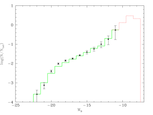
Figure 3: B–band luminosity function of cluster galaxies as predicted by our “best case” cluster model versus the observational data (by Trentham 1998). Left panel: results for galactic models with the PNJ IMF. Right panel: results for galactic models with the Salpeter IMF.

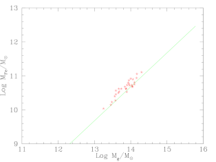
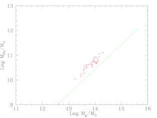
Figure 4: Metallicity (iron abundance) of the ICM as predicted by our chemical evolution model for the cluster versus the observational data (by Matsumoto et al. 2000). Left panel: results for galactic models with the PNJ IMF. Right panel: results for galactic models with the Salpeter IMF.

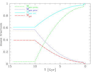
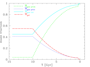
Figure 5: Time evolution of the cluster components: mass in primordial and processed gas separately, total gas mass, and mass in galaxies. Left panel: results for galactic models with the PNJ IMF. Right panel: results for galactic models with the Salpeter IMF.

Although the predicted LF is virtually the same in the two models, strong differences are found in the predicted gas and metallicity content in the ICM. Fig. 4 shows the predicted abundances in the ICM in the PNJ and Salpeter case (left and right panel, respectively). In the plot, lines of unit slope represent iso-metallicity loci. Observational data roughly fall onto the same abundance level, around 0.3 $Z_{\odot}$. It is evident how adopting galactic models with the PNJ IMF improves predictions about the metallicity of the ICM.

Fig. 5 shows the evolution of the mass fraction of the various components of the cluster: the primordial gas, which gets consumed by galaxy formation; the processed gas, namely the gas that has been processed inside galaxies and then re-ejected as GW; the total gas, sum of the primordial and of the processed gas; the mass in galaxies, that is in the stellar component we see today, “left over” after the GW. While in the Salpeter case (right panel) the overall mass that remains locked into galaxies (red line) is larger that the mass ejected in the GWs (dark blue line), the opposite is true in the cluster model with the PNJ galaxies (left panel), as qualitatively expected from the comparison of the different galactic models in § 2.2. In the latter case, the mass of the re-ejected gas is $\sim 1.5$ times larger than that locked into galaxies. Although this is not enough to account for the whole of the observed intra-cluster gas (whith a mass 2–5 times larger than that in galaxies, Arnaud et al. 1992), the amount of gas re-ejected by galaxies is expected to make up for a remarkable fraction of the overall ICM.

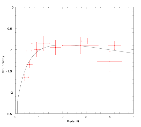
Figure 6: Galactic Formation Rate with a functional form following the Madau–plot. Data Steidel et al. (1999).

5 A Madau–like GFR

In the previous “best case” model the GFR was calibrated so as to reproduce the observed LF, being otherwise arbitrary. An alternative recipe for the GFR is a functional form resembling the cosmic SFR of the Madau–plot (Fig. 6). The burst of dwarf galaxy formation at $z\sim 10-20$ is always needed to reproduce the faint end of the LF, but this is not in constrast with the Madau–plot.

Fig. 7 shows the corresponding predictions for metallicity, metallicity evolution and mass fraction evolution of the various components. Only results for galactic models with the PNJ IMF are shown; the comparison with the corresponding Salpeter case would lead to considerations similar to those in § 4. Once more, the average metallicity of the observed clusters is quite well reproduced, and a large amount of gas ($\sim$1.5 times the mass in galaxies) is predicted to be re-ejected by GWs. With this Madau–like form of the GFR, however, it is hard to reproduce the observed LF in detail.

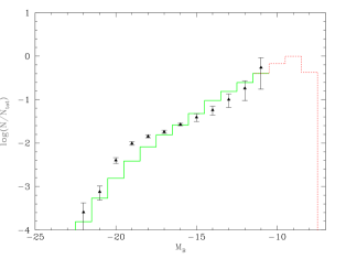
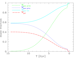
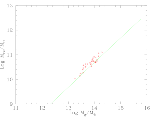
Figure 7: Results for the cluster model adopting a Madau–like GFR and galactic models with the PNJ IMF. Top left: luminosity function. Top right: time evolution of the mass fraction in the different cluster components. Bottom left: present day iron abundance in the ICM. Bottom right: redshift evolution of the iron abundance in the ICM; data by Matsumoto et al. (2000), Fukazawa et al. (1998), Mushotzky & Loewenstein (1997).

6 Summary and conclusions

Galactic winds from elliptical galaxies are the most likely source of the chemical enrichment of the ICM. In this scenario, various studies in literature suggests that a non–standard IMF must be invoked for elliptical galaxies, if we are to account for the metal pollution of the ICM (§ 1).

We considered GW models for ellipticals adopting a variable, physically grounded IMF whose behaviour in time and space follows common expectations for the Jeans mass. This IMF (by PNJ) naturally predicts a lower locked–up fraction in the early galactic stages, especially for massive ellipticals and/or for high redshifts of formation. Galactic models calculated with this IMF have been shown to reproduce successfully a variety of observational properties of ellipticals (Chiosi et al. 1998). In this paper we discussed the resulting GW ejecta for these model ellipticals with respect to models adopting the standard Salpeter IMF. Our new models predict galaxies to eject both more metals and more gas than standard chemical models do (§ 2).

Then we have developed a toy–model for the chemical evolution of the ICM, following the formation history of cluster galaxies and the corresponding chemical evolution of the ICM in a self–consistent fashion. The model can adopt different sets of galactic models in turn, so as to explore the corresponding variation of the predicted metal pollution history of the ICM (§ 3).

The galaxy formation history can be calibrated so as to reproduce the observed present–day LF of cluster galaxies. A good match with the LF can be obtained both using model ellipticals with the PNJ IMF, and using more standard galactic models with the Salpeter IMF. However, when the PNJ galactic models (also favoured on the base of their spectro–photometric properties) are adopted, predictions on the metal abundances of the ICM are remarkably improved. With these models, the mass of gas re-ejected in the GWs exceeds the mass stored in stars by a factor of 1.5, and becomes an important fraction of the total intra-cluster gas (§ 4).

We also explored an alternative cluster model, where the galactic formation history follows the trend suggested by the Madau plot (at the expence of a less successful prediction on the LF). Conclusions about the chemical evolution of the ICM, with the PNJ IMF, do not substantially change: the model predicts the correct metal abundance of the ICM, and suggests that an important fraction of the intracluster gas may be of galactic origin (§ 5).

References

References

- [1] Arimoto N., Yoshii Y., 1987, A&A 173, 23
- [2] Arnaud M., Rothenflug R., Boulade O., Vigroux L., Vangioni-Flam E., 1992, A&A 254, 49
- [3] Bica E., Bonatto C., Pastoriza M.G., Alloin D., 1996, A&AS 313, 405
- [4] Bressan A., Chiosi C., Fagotto F., 1994, ApJS 94, 63
- [5] Chiosi C., 2000, A&A 364, 423
- [6] Chiosi C., Bressan A., Portinari L., Tantalo R., 1998, A&A 339, 355
- [7] David L.P., Forman W., Jones C., 1991, ApJ 380, 39
- [8] De Young D.S., 1978, ApJ 223, 47
- [9] Elbaz D., Arnaud M., Vangioni–Flam E., 1995, A&A 303, 345
- [10] Fukazawa Y., Makishima K., Tamura T., Ezawa H., Xu H., Ikebe Y., Kikuchi K., Ohashi T., PASJ 50, 187
- [11] Gibson B.K., Matteucci F., 1997a, ApJ 475, 47
- [12] Gibson B.K., Matteucci F., 1997b, MNRAS 291, L8
- [13] Himmes A., Biermann P., 1980, A&A 86, 11
- [14] Larson R.B., 1974, MNRAS 169, 229
- [15] Larson R.B., 1986, MNRAS 218, 409
- [16] Larson R.B., 1998, MNRAS 301, 569
- [17] Larson R.B., Dinerstein H.L., 1975, PASP 87, 911
- [18] Loewenstein M., Mushotzky R.F., 1996, ApJ 466, 695
- [19] Martinelli A., Matteucci F., Colafrancesco S., 1998, MNRAS 298, 42
- [20] Martinelli A., Matteucci F., Colafrancesco S., 2000, A&A 354, 387
- [21] Matsumoto H., Tsuru T.G., Fukazawa Y., Hattori M., Davis D.S., 2000, PASJ 52, 153
- [22] Matteucci F., 1992, ApJ 397, 32
- [23] Matteucci F., 1994, A&A 288, 57
- [24] Matteucci F., 1997, Fund. Cosmic Phys. 17, 283
- [25] Matteucci F., Gibson B.K., 1995, A&A 304, 11
- [26] Matteucci F., Vettolani G., 1988, A&A 202, 21
- [27] Mitchell R.J., Culhane J.L., Davidson P.J.N., Ives J.C., 1976, MNRAS 176, 29
- [28] Moretti A., Portinari L., Chiosi C., 2001, in preparation
- [29] Mori M., Burkert A., 2000, ApJ 538, 559
- [30] Mushotzky R., Loewenstein M., 1997, ApJ 481, L63
- [31] Mushotzky R., Loewenstein M., Arnaud K.A., Tamura T., Fukazawa Y., Matsushita K., Kikuchi K., Hatsukade I., 1996, ApJ 466, 686
- [32] Nath B.B., Chiba M., 1995, ApJ 454, 604
- [33] Padoan P., Nordlund A.P., Jones B.J.T., 1997, MNRAS 288, 145 (PNJ)
- [34] Pagel B.E.J., 1997, Nucleosynthesis and chemical evolution of galaxies, Cambridge University Press
- [35] Renzini A., 1997, ApJ 488, 35
- [36] Renzini A., Ciotti L., 1993, ApJ 416, L49
- [37] Scalo J., Vazquez-Semadeni E., Chappell D., Passot T., 1998, ApJ 504, 835
- [38] Serlemitsos P.J., Smith B.W., Boldt E.A., Holt S.S., Swank J.H.,1977, ApJ 211, L63
- [39] Steidel C.C., Adelberger K.L., Giavalisco M., Dickinson M., Pettini M., 1999, ApJ 519, 1
- [40] Tantalo R., Chiosi C., Bressan A., 1998, A&A 333, 419
- [41] Tegmark M., Silk J., Rees M.J., Blanchard T., Abel T., Palla F., 1997, ApJ 474, 1
- [42] Tinsley B.M., 1980, Fund. Cosmic Phys. 5, 287
- [43] Trentham N., 1994, Nature 372, 157
- [44] Trentham N., 1998, MNRAS 294, 193
- [45] Vigroux L., 1977, A&A 56, 473
- [46] White S.D.M., Rees M.J., 1978, MNRAS 183, 341
- [47] Worthey G., Dorman B., Jones L.A., 1996, AJ 112, 948
- [48] Zepf S.E., Silk J., 1996, ApJ 466, 114