The Spectra of Red Quasars

Paul J. Francis ^1,2 Catherine L. Drake ¹ Matthew T. Whiting ³ Michael J. Drinkwater ³ Rachel L. Webster ³

Abstract

We measure the spectral properties of a representative sub-sample of 187 quasars, drawn from the Parkes Half-Jansky, Flat-radio-spectrum Sample (PHFS). Quasars with a wide range of rest-frame optical/UV continuum slopes are included in the analysis: their colours range from $2<B-K<7$ . We present composite spectra of red and blue subsamples of the PHFS quasars, and tabulate their emission-line properties.

The median H $\beta$ and [O III] emission-line equivalent widths of the red quasar sub-sample are a factor of ten weaker than those of the blue quasar sub-sample. No significant differences are seen between the equivalent width distributions of the C IV, C III] and Mg II lines. Both the colours and the emission-line equivalent widths of the red quasars can be explained by the addition of a featureless red synchrotron continuum component to an otherwise normal blue quasar spectrum. The red synchrotron component must have a spectrum at least as red as a power-law of the form $F_{\nu}\propto\nu^{-2.8}$ . The relative strengths of the blue and red components span two orders of magnitude at rest-frame 500nm. The blue component is weaker relative to the red component in low optical luminosity sources. This suggests that the fraction of accretion energy going into optical emission from the jet is greater in low luminosity quasars. This correlation between colour and luminosity may be of use in cosmological distance scale work.

This synchrotron model does not, however, fit $\sim 10$ % of the quasars, which have both red colours and high equivalent width emission-lines. We hypothesise that these red, strong-lined quasars have intrinsically weak Big Blue Bumps.

There is no discontinuity in spectral properties between the BL Lac objects in our sample and the other quasars. BL Lac objects appear to be the red, low equivalent width tail of continuous distribution. The synchrotron emission component only dominates the spectrum at longer wavelengths, so existing BL Lac surveys will be biassed against high redshift objects. This will affect measurements of BL Lac evolution.

The blue PHFS quasars have significantly higher equivalent width C IV, H $\beta$ and [O III] emission than a matched sample of optically selected QSOs.

¹ Research School of Astronomy and Astrophysics, Australian National University, Canberra ACT 0200
pfrancis,cdrake@mso.anu.edu.au
² Joint appointment with the Department of Physics, Faculty of Science, Australian National University
³ School of Physics, University of Melbourne, Victoria 3010
mwhiting, m.drinkwater, rwebster@physics.unimelb.edu.au

Keywords: Quasars: general — Quasars: Emission Lines — BL Lacertae Objects: General

1 INTRODUCTION

The rest-frame optical/UV emission of radio quiet QSOs is dominated by strong broad emission lines and by extremely blue continuum emission (the Big Blue Bump, which peaks in the far-UV, eg. Malkan & Sargent 1982). The emission of flat radio spectrum radio-loud quasars is often quite different. It is now well established that many have much redder colours than traditional optically selected QSOs (eg. Rieke, Lebofsky & Wisniewski 1982, Webster et al. 1995). A few also have extremely low equivalent width emission lines, and are known as BL Lac objects.

What is responsible for these differences? In this paper, we address this question, using the spectra of a representative sub-set of flat radio spectrum sources from the Parkes Half-Jansky Flat-Spectrum survey (PHFS). This survey consists of 323 sources with flux densities at 2.7 GHz of greater than 0.5 Jy, and radio spectral indices $\alpha$ ( $F_{\nu}\propto\nu^{\alpha}$ ) with $\alpha>-0.5$ as measured between 2.7 and 5.0 GHz (Drinkwater et al. 1997). The PHFS quasars lie at redshift $0<z<4$ .

Francis, Whiting and Webster (2000, hereafter FWW) obtained quasi-simultaneous optical and near-IR photometry for a random subset of 157 PHFS sources. They showed that the spectral energy distributions of red quasars are diverse. They divided the sources, on the basis of their colours, into three classes.

1.

Dusty quasars. About 10% of the sample fall into this category. They have the strongly curved spectral energy distributions expected from dust obscuration, and show reddened line ratios. Their spectra are discussed by FWW.
2.

Galaxies. Another 10% of the sources are spatially resolved, and have spectra typical of elliptical galaxies. These sources are discussed by Masci, Webster and Francis (1997).
3.

Pseudo power-law sources. About 80% of the sources have approximately power-law spectral energy distributions, extending from the rest-frame UV to the near IR. These power-law continua vary in slope between $F_{\nu}\propto\nu^{\sim 0}$ and $F_{\nu}\propto\nu^{\sim-2}$ . These are the sources we discuss in this paper.

What are these pseudo power-law sources, and what is responsible for their diversity of continuum slopes? Three models have been proposed. Firstly, red pseudo-power-law sources might have intrinsically weaker Big Blue Bumps (eg. McDowell et al. 1989). Secondly, all quasars might have similar Big Blue Bumps, but in the redder quasars this emission might be partially absorbed by dust (eg. Webster et al. 1995). The dust properties would have to be unusual not to induce curvature in the spectra. Thirdly, all quasars might have similar Big Blue Bumps, but in the redder quasars, this Big Blue Bump emission is swamped by a red synchrotron emission component from the radio jet (eg. Serjeant & Rawlings 1997).

In this paper, we test these models against the spectra of the PHFS pseudo power-law sources. In Section 2 we discuss our spectra of the PHFS quasars, and show that they represent a reasonably representative sub-sample. In Section 3 we describe in detail our measurements of the spectra, and in Section 4 we show the results. The predictions of the three models for the emission-line properties are discussed in Section 5. We show, in Section 6, that the spectra are mostly consistent with the synchrotron model, and derive constraints on this model. Finally, conclusions are drawn in Section 7.

2 The Sample

We obtained spectra for 77 of the PHFS sources with the Anglo-Australian Telescope (AAT) and the Siding Spring 2.3m telescope (Drinkwater et al. 1997). These were combined with 25 unpublished spectra drawn from the AAT archives, and 86 spectra drawn from the compilation of Wilkes et al. (1983). We thus have spectra of 187 of the 323 sources in the PHFS.

In Fig 1, we show the number of PHFS sources for which we have spectra as a function of $B_{J}$ magnitude. Note that the fraction with spectra is reasonably uniform.

Refer to caption — Figure 1: The number of PHFS sources as a function of $B_{J}$ magnitude (solid line, left axis) and the percentage of PHFS sources for which we have digital spectra (dotted line, right axis). Sources for which we only have an upper limit on their $B_{J}$ magnitude are shown in the right panel.

The quality and wavelength coverage of the spectra is very diverse. The signal to noise ratio of most quasars was too poor to allow measurements of line widths or profiles. As most are not spectrophotometric, we did not attempt to extract continuum parameters or line ratios from the spectra. The quality and diversity of the spectra can best be appreciated by looking at the sample spectra in Drinkwater et al. (1997).

2.1 Sub-samples

Spatially extended sources were excluded from this paper. Images from the UK Schmidt and Palomar sky survey images (IIIa-J) were automatically classified, using the COSMOS and APM scanners. The automated classification was checked against our own deeper imaging. We classified 18 of the PHFS sources with spectra as spatially extended: they are discussed by Masci et al. (1997).

The remaining point-like sources were analysed on the basis of their optical/near-IR colours. The quasi-simultaneous broad-band magnitudes of FWW were used. This excluded half of the quasars with spectra, as no photometry was available for them. Sources with $B-I>2.6$ were excluded from the analysis. These sources have the convex continuum spectral energy distributions expected from dust absorption, and their spectra were discussed in FWW.

In Fig 2 we show the percentage of these remaining pseudo power-law sources for which we have spectra, as a function of their $B-K_{n}$ colour. Note once again that the subsample with spectra is reasonably representative.

We defined two subsamples of these pseudo-power-law sources. They were defined on the basis of their rest-frame colours. We measured these colours from our broad-band photometry, and not from the (non-spectrophotometric) spectra. The flux densities at 340nm and 750nm were calculated by extrapolation between the photometric data points from FWW.

•

The Blue Sample. 22 sources with spectra. Flux density ( $F_{\lambda}$ ) at rest-frame 340nm which exceeds that at 750nm by more than 0.45 dex (a factor of 2.8)
•

The Red Sample. 20 sources with spectra. Flux density ratio of less than 0.45 dex between these wavelengths.

This dividing line corresponds to a power-law of index $F_{\nu}\propto\nu^{-0.7}$ between these two wavelengths, and was chosen to bisect the sample.

As a control sample, the Large Bright QSO Sample (LBQS) was used (Morris et al. 1991 and refs. therein). This sample of 1053 optically selected QSOs is well matched in both redshift and optical luminosity to the PHFS. Broad absorption line QSOs were excluded from the comparison.

3 Analysis

Error arrays were not available for most of the sample spectra. We therefore estimated them as follows. For each pixel, we fit a straight line to the fluxes in the 15 pixels centred on it. The sum of the squares of the residuals from this fit was divided by 13 to estimate the error variance in the pixel. We divided by 13 rather than 15 to allow for the two degrees of freedom in the straight-line fit.

We iteratively fit a 4th order Chebyshev polynomial to the continuum of each quasar. Wavelength regions with strong emission-lines were excluded from the fitting. The fits were iterated three times, with regions more than $2\sigma$ above or $4\sigma$ below each fit excluded from the next. The results were checked by eye: these fits were subjectively judged to be good for 95% of the quasars. The remaining 5% were fit interactively.

Emission-line equivalent widths were obtained by dividing the flux above these continuum fits by the continuum level, integrated over the wavelength regions in Table 1. Only the strongest emission-lines were measured, as the signal-to-noise ratio was too poor to allow measurement of the weaker lines. Ly $\alpha$ was not measured due to the difficulty in defining the continuum under it, and the small number of red quasars at high enough redshift. The [O III] equivalent widths are for the stronger component (the 500.7 nm line) only. All the continuum fits and line equivalent widths were checked by eye, and about 10% of the automated measurements were replaced with interactive ones.

Table 1: Emission-line Integration Limits

Line	Lower Rest Wavelength Limit	Upper Rest Wavelength Limit
C IV	149 nm	159 nm
C III]	183 nm	196 nm
Mg II	268 nm	290 nm
H $\beta$	476 nm	493 nm
$[$ O III $]$	498 nm	505 nm

Composite quasar spectra were obtained as follows. Each individual spectrum was divided through by the continuum fit and shifted to its rest-frame, using interactively defined redshifts. The spectra were then rebinned and co-added. All spectra were equally weighted in the co-add, regardless of their signal-to-noise ratio. This degrades the signal-to-noise ratio of the final composite spectrum, but ensures that it is not biassed towards the properties of the quasars with better quality spectra. The fluxes at very blue and very red wavelengths were given a low weighting, to reflect their generally poor signal-to-noise ratios. Only wavelength regions to which at least five individual quasars contributed were included in the composite spectra.

3.1 Sources without Redshifts

Three sources have no redshift in Drinkwater et al. (PKS 0048 $-$ 097, PKS 0829 $+$ 046 and PKS1156 $-$ 094). Falomo (1991) measured a redshift of 0.18 for PKS 0829 $+$ 046, which we adopt. Both the other sources have red colours and would lie in the red sample regardless of their redshift.

We estimated upper limits on the emission-line equivalent widths of PKS 0048 $-$ 097 and PKS 1156 $-$ 094 as follows. The biggest wavelength gap between strong emission lines is between Mg II and H $\beta$ . The ratio of their wavelengths is 1.74. Thus any wavelength range with an end wavelength more than 1.74 times its starting wavelength must contain at least one strong line. In both spectra, the least noisy wavelength range of this width was taken. The $3\sigma$ limit for a line of width $5000{\rm km\ s}^{-1}$ was computed as a function of wavelength throughout this region, and the highest value taken as our limit.

We place a $3\sigma$ upper limit of 0.17nm for PKS 0048 $-$ 097. The spectrum of PKS 1156 $-$ 094 is poor, and we can only place a $3\sigma$ upper limit of 6.6nm on the equivalent width of any emission line.

3.2 Luminosities and Rest-frame Colours

Continuum luminosities were calculated at particular rest-frame wavelengths, by linear extrapolation between adjacent redshifted photometric bands from FWW. We assume that $H_{0}=70{\rm km\ s}^{-1}{\rm Mpc}$ , $\Omega_{\rm matter}=0.3$ and $\Omega_{\Lambda}=0.7$ throughout. Radio luminosities were calculated in the same way, using radio flux densities at 1600, 2468, 4800 and 8640 MHz obtained by Webster et al. (in preparation). Emission-line luminosities were calculated by scaling the spectra to match the broad-band photometry of FWW extrapolated to the line wavelength.

4 Results

4.1 Composite Spectra

The composite spectra of blue and red PHFS quasars (excluding the two without measured redshifts), and of the optically selected LBQS QSOs, are shown in Figs 3 and 4. A number of differences can be seen. The red PHFS composite has much weaker Mg II, Balmer and [O III] lines than the blue PHFS composite. The C III] and C IV lines, however, are more similar in strength. The LBQS composite more closely resembles the blue PHFS composite, but its Ly $\alpha$ , C IV, H $\beta$ and [O III] lines are weaker. The reality of these differences will be addressed in the next section.

4.2 Equivalent Width Measurements

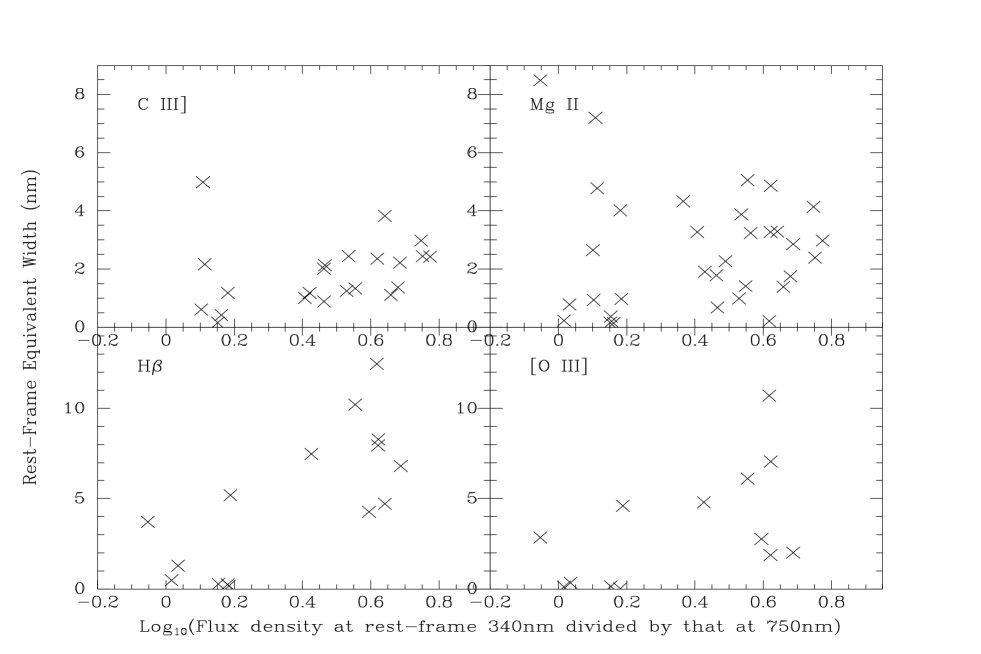
The equivalent width measurements can be found in a machine readable table, included in the electronic edition of this paper. Equivalent widths are plotted against continuum slope in Fig 5. Histograms of equivalent widths for the blue and red sub-samples, and for the LBQS, are shown in Figs 6, 7 and 8. The two PHFS quasars without measured redshifts (both in the red sample) are not included.

Are the differences between the red and blue sub-samples real? The correlation between the equivalent width of H $\beta$ and the continuum slope is significant at the 99.2% level, using Spearman’s Rank Correlation test. A Kolmogorov-Smirnov test confirms that the H $\beta$ equivalent width distributions of the two sub-samples are different at the 97% confidence level. The C III] equivalent width distributions are marginally inconsistent (at the 95% level). There are no other differences significant at the 95% confidence level.

The two quasars without measured redshifts were excluded from this analysis. If we assume that they are of low enough redshift that H $\beta$ would have been seen, they increase the significance of the difference.

4.3 Line Ratios

No correlation was found between line flux ratios and colour. The correlation predicted by a dust model is, however, weak enough to be consistent with the observations. We have wide wavelength coverage, spectrophotometric spectra for three of the reddest pseudo power-law sources, however, from which we can measure Balmer decrements. In all three, the ratio of H $\alpha$ to H $\beta$ is around 3.5, consistent with no dust reddening.

4.4 Correlations with Luminosity

The continuum slope of the PHFS samples correlates with the optical continuum luminosity (Fig 9). Spearman’s Rank Correlation Test shows that this correlation is significant with 99.999% confidence. No significant correlation is seen between continuum slope and radio luminosity.

As the PHFS is a flux limited sample, redshift and luminosity are strongly correlated. Is this really a correlation against luminosity, or could it be a correlation against redshift? To test this, the sample was subdivided into redshift bins. The median luminosity of the sources in each bin was calculated, and subtracted from all the sources in that bin. The resultant differential luminosities still correlated with colour, with 95% confidence. When the process was repeated with luminosity bins, no significant residual correlation was seen. We therefore conclude that the physical correlation is between colour and luminosity.

A stronger correlation is seen between the emission-line luminosity and the continuum slope (Fig 10). The correlation with C III] luminosity is only significant at the 97% level, but the other correlations shown are significant with 99.99% confidence or better.

5 Models

5.1 Weak Blue Bump

How should the strength of the Big Blue Bump affect the emission-line properties? The Big Blue Bump is normally ascribed to thermal emission from an accretion disk. The disk could be different in red and blue quasars. Alternatively, the rest-frame UV/optical emission may be entirely synchrotron. Red and blue quasars could have different electron energy spectra in the jet. Either way, the emission-lines of red and blue quasars should be quite different, as the Big Blue Bump emission dominates their photoionisation.

We modelled the effect of varying the Big Blue Bump size on the emission line, using the Cloudy photoionisation code (Ferland 1996). The broad emission-line region was modelled as a single plane-parallel slab of uniform hydrogen number density $3.1\times 10^{16}{\rm m}^{-3}$ , and solar metallicity. The flux incident on the front of the slab at 500nm wavelength was fixed at $F_{\nu}=1.0\times 10^{-9}{\rm W\ Hz}^{-1}$ (low ionisation model), $F_{\nu}=6.3\times 10^{-9}{\rm W\ Hz}^{-1}$ (medium ionisation model) and $F_{\nu}=4.0\times 10^{-8}{\rm W\ Hz}^{-1}$ (high ionisation model). All these parameters are typical of published broad-line region models.

Cloudy’s standard AGN photoionising continuum was used. This is a power-law in the UV and optical, with exponential upper- and lower cut-offs, together with a second power-law in the X-rays:

f_{\nu}=\nu^{\alpha_{\rm UV}}e^{\frac{-h\nu}{kT_{\rm BB}}}e^{\frac{-kT_{\rm IR}}{h\nu}}+a\nu^{\alpha_{\rm X}}

where $T_{\rm BB}=150,000$ K, $kT_{\rm IR}=0.01$ Ryd and $\alpha_{\rm X}=-1$ . The constant $a$ is set such that the slope of a power-law extrapolated between 2 keV and 250nm rest-frame, $\alpha_{OX}$ , is $-1.4$ . Thus the hard X-ray fluxes of red and blue quasars are same, as suggested by the ROSAT observations of Siebert et al. (1998).

All that we varied was the strength of the Big Blue Bump, parameterised by $\alpha_{\rm UV}$ . The equivalent widths of the strongest emission lines were calculated as a function of $\alpha_{\rm UV}$ , for each of the three ionisation models. Results are shown in Fig 11.

A few clear patterns emerge. H $\beta$ is weaker in weak bump quasars. This is expected, as it is predominantly photoionised by flux just shortward of the Lyman limit, which is dominated by the Big Blue Bump. C III] and C IV can be either weaker or stronger in weak bump quasars, depending on the ionisation state of the broad-line region. This too is expected, as the strength of the Big Blue Bump affects the ionisation parameter, and hence the population of the different ionisation states of carbon. Mg II becomes much stronger in weak bump quasars. Mg II is a relatively low ionisation line, and is predominantly excited by X-rays penetrating deep into the emission-line clouds. Thus an ionising continuum weak in UV photons but relatively strong in harder X-rays is ideal for Mg II formation.

A more realistic model would allow for the stratified nature of the emission-line regions. It is also unlikely that the physical properties of the emission line region are uncorrelated with the colour of the continuum emission.

5.2 Dust

Normal dust models predict a strongly curved continuum in red quasars, and hence are not consistent with the photometry of the pseudo power-law sources (FWW). If the dust were deficient in small grains, however, the UV absorption would be reduced, and the predicted continuum emission could be brought into agreement with that observed.

Dust should affect the emission-line ratios, but should not affect the emission-line equivalent widths, as it should absorb line and continuum radiation equally. The exception to this would be where the dust is either patchy on scales comparable to the broad-line region, or where it is mixed in with the broad-line region.

5.3 Synchrotron Emission

Unified models suggest that we are observing flat radio spectrum quasars from close to the axis of their jets. Any emission from these jets would thus be relativistically boosted. If these jets sometimes emitted a synchrotron component with very red colours in the optical, it could produce the red colours. Whiting, Webster & Francis (2001, hereafter WWF) showed that a model of the continuum emission with two components (a big blue bump and a red synchrotron component) can reproduce the colours of the pseudo power-law sources as measured by FWW, including the small (but significant) deviations from a pure power-law. The model also correctly predicts the polarisation properties of the small fraction of PHFS quasars for which this data is available.

If the synchrotron model is correct, there should be an anti-correlation between the equivalent widths of the emission lines and the redness of the continuum emission. This is because the emission-line flux of a quasar should be proportional to the strength of the Big Blue Bump that photoionises it, and should not be affected by the strength of any red synchrotron emission component. The red component will have too little flux in the UV to ionise emission lines, and it is probably beamed, and hence will only illuminate a small part of the emission-line region. Thus if the observed red continuum emission greatly exceeds the big blue bump, it will also greatly exceed the fluxes of the emission lines, which will hence have very low equivalent widths. The effect should be most marked for longer wavelength lines, as the red synchrotron component will be relatively stronger at longer wavelengths. Line ratios should not correlate with colour.

6 Discussion

At short wavelengths, there are no significant differences between the emission-line equivalent widths of the red and blue sub-samples. H $\beta$ , however, shows a very significant difference, in the sense that most red sources have very weak lines. The data from [O III] are also consistent with this (Table 2).

Table 2: Median Equivalent Widths

Line	Blue PHFS Quasars	Red PHFS Quasars	Ratio Blue/Red
C IV	3.3 nm	2.7 nm	1.2
C III]	2.2 nm	1.1 nm	2.0
Mg II	2.6 nm	2.3 nm	1.2
H $\beta$	7.9 nm	0.9 nm	9.1
$[$ O III $]$	4.4 nm	0.4 nm	12.6

These results are consistent with the red synchrotron component model, if this red component is about ten times stronger than the blue component at $\sim 500$ nm wavelength, but no longer swamps the blue component at 300nm. This implies a spectrum at least as red as a power-law of the form $F_{\nu}\propto\nu^{\sim-2.8}$ , which is consistent with the theoretical modelling of WWF.

These results are not consistent with the dust model, which predicts no correlation between equivalent width and colour. Neither are they consistent with the weak Blue Bump model, which predicts that Mg II should be stronger in the red quasars, and that H $\beta$ should only be weaker by a factor of $\sim 3$ , not $\sim 10$ .

Let us therefore assume that the weakness of the lines of the red sub-sample is due primarily to dilution by a red synchrotron component. We detect the H $\beta$ line at $3\sigma$ confidence or better in all but one of the red quasars with decent data. The equivalent widths span roughly two orders of magnitude at rest frame 500nm, with no obvious bimodality. In at most 10% of the red quasars can the red continuum component exceed the blue component by a factor of more than 100, at rest-frame 500nm. This too is consistent with the modelling of WWF.

6.1 Red, Strong-Lined Quasars

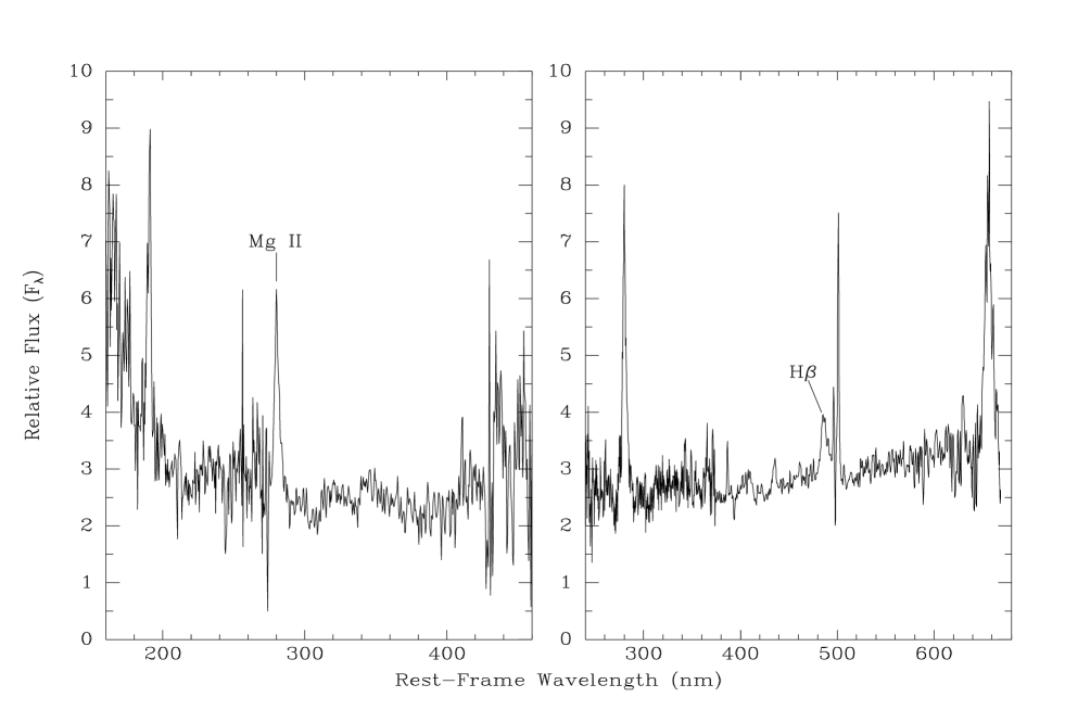
If the synchrotron model is correct, all red quasars should have low equivalent width emission-lines, and all quasars with very low equivalent widths should be red. The latter is consistent with our data, but as Fig 5 shows, there are a small number of extremely red quasars with high equivalent width Mg II lines. The spectra of the two most extreme red, strong-lined quasars are shown in Fig 12. Indeed, these red quasars have the highest equivalent width Mg II emission-lines in the sample.

These sources clearly do not fit into the simple synchrotron model. Dust could redden the continuum without changing the equivalent widths. The Balmer decrements of these sources are, however, $\sim 3.5$ , which is typical of unreddened AGN.

A weak Big Blue Bump model fits the red colours and high Mg II equivalent widths of these sources well. We therefore hypothesise that these quasars have intrinsically weak Big Blue Bumps. Note, however, that while the equivalent widths of these sources are anomalous, their line luminosities fit on the correlation with continuum slope (Fig 10).

6.2 The Correlation between Luminosity and Continuum Slope

The synchrotron model appears to best fit most of the spectra. What then determines the relative strength of the synchrotron and Big Blue Bump components, and hence the quasar colours? The continuum slope measured between 340 and 750nm should be a good measure of the relative strength of the synchrotron and Big Blue Bump components. Emission-line luminosities should correlate strongly with the luminosity of the Big Blue Bump which photoionises them. Thus the correlations shown in both Figs 9 and 10 suggest that the ratio of synchrotron emission to Big Blue Bump flux is relatively high in quasars with low luminosity Big Blue Bumps.

This implies that in quasars with low luminosity Big Blue Bumps, the fraction of the accretion energy going into the jet is relatively high, or that the jet emission extends to shorter wavelengths in these sources. The $1\sigma$ scatter in this correlation is 0.4 dex, which is better than the scatter in the Baldwin Effect. This correlation may thus be useful for cosmological distance scale work.

6.3 Implications for BL Lac Objects

BL Lac objects are normally defined as having no observed emission lines with rest-frame equivalent widths greater than 0.5nm (eg. Stickel et al. 1991, Rector et al. 2000). In our model, this implies that the red synchrotron emission component exceeds the blue one at the line wavelength by a factor of $\sim 10$ .

We do not see any bimodality in the distribution of equivalent factors, though our sub-sample is small. If confirmed, this would imply that radio selected BL Lac objects are simply the tail of the normal population of flat radio spectrum quasars, and not a different class with intrinsically weaker emission lines.

Our analysis suggests that the synchrotron emission component is very red, and hence that it dilutes long wavelength lines far more effectively than short wavelength lines. This implies that BL Lac samples are biassed against finding high redshift objects.

How significant could this bias be? Consider a model in which the red continuum component has a spectrum of the form $F_{\nu}\propto\nu^{-2.8}$ , and the logarithm of the ratio of red to blue components at the wavelength of H $\beta$ is uniformly distributed between 0 and 2, as suggested by our observations. The ratio of red to blue components at the wavelength of Mg II will be 3.4 times smaller than at H $\beta$ , while at C III] it will be 7.8 times smaller. It is assumed that the ratio of red to blue components does not correlate with redshift or luminosity.

Now consider, for example, a sample of BL Lac objects chosen on the basis of spectra covering 400 — 600nm. At redshift zero, the strongest line in this wavelength range will be H $\beta$ , which in blue PHFS quasars has a rest-frame equivalent width of $\sim 5$ nm. For this line to have an observed equivalent width of less than 0.5nm, we require that the red component at the wavelength of H $\beta$ exceed the blue component by a factor of ten. According to our model, 50% of all red quasars meet this criterion and would hence be classed as BL Lac objects.

At redshift one, however, Mg II will be the strongest line within this observed wavelength region. In blue PHFS quasars, Mg II has a median rest-frame equivalent width of 3nm. For the line to have a rest-frame equivalent width of less than 0.5nm, we require that the red continuum component exceed the blue one by a factor of 6 at the wavelength of Mg II. This implies that the red component must exceed the blue by a factor of $3.4\times 6=20$ at the wavelength of H $\beta$ . According to our model, only 35% of red quasars will meet this criterion. Repeating this calculation at redshift two (where C IV is the strongest line), only 6% of red PHFS quasars would be classed as BL Lac objects.

Thus any sample using spectra at a uniform observed-frame wavelength will miss $\sim 30$ % of the BL Lacs at redshift one, and $\sim 90$ % at redshift two. Our small sub-sample size makes these estimates highly uncertain. Nonetheless, this is probably sufficient to cancel out the negative evolution claimed by some authors (eg. Rector et al. 2000), but not to match the enormous positive evolution seen in other classes of quasar.

6.4 Differences between Radio-Loud and Radio-Quiet Quasars

It has long been known that the optical spectra of radio-loud and radio-quiet quasars are remarkably similar, despite the enormous difference in their radio luminosities. A number of small differences in the emission-line properties have been claimed (eg. Boroson & Green 1992, Francis, Hooper & Impey 1993, Corbin & Francis 1994, Corbin 1997), but only on the basis of small, poorly matched and/or incomplete samples. These studies found that C IV, C III] and [O III] had higher equivalent widths in flat radio spectrum quasars than in radio-quiet quasars.

The optical luminosity and redshift distribution of the LBQS are quite similar to those of the PHFS quasars, so any differences between the emission-lines of the two samples must be physical. If we compare the spectra of the LBQS QSOs with the blue PHFS sub-sample, we find that the equivalent width distributions of C IV, H $\beta$ and [O III] are significantly different, with 95% confidence. C III] is different with 94.8% confidence. In all cases, the equivalent widths of the blue PHFS quasars are greater than those of the LBQS QSOs. The red PHFS quasars have significantly weaker Mg II and H $\beta$ equivalent widths than the LBQS QSOs, presumably due to dilution by the red synchrotron component.

7 Conclusions

We conclude that the spectra of the red PHFS quasars are significantly different from those of the blue PHFS quasars. Small number statistics make our conclusions tentative, though they are formally significant. The probable differences are consistent with a model in which the red colours are due to the addition of a featureless red synchrotron continuum component to an otherwise normal blue quasar spectrum, as proposed by WWF. The red component must have a spectrum at least as red as a power-law of the form $F_{\nu}\propto\nu^{-2.8}$ . This red component contributes no more than half the continuum flux at rest-frame 300nm, but at rest-frame 500nm it contributes about 90% of the continuum flux of the red quasars. The physics of such a component is discussed by WWF.

The relative strengths of the blue and red components span two orders of magnitude at rest-frame 500nm. The blue component is relatively weaker in low optical luminosity sources.

If this model is correct, then existing BL Lac surveys are biassed against high redshift objects, though this bias is insufficient to bring the evolution of BL Lacs into consistency with the evolution of other quasars.

A few PHFS quasars, however, have both very red colours and very high equivalent width emission-lines. These quasars do not easily fit the synchrotron model, but their properties can be fit by an intrinsically weak Big Blue Bump model. We confirm that the emission-lines of optically selected QSOs have significantly weaker equivalent widths than those of radio-loud, flat radio spectrum quasars with similar optical luminosities.

Digital copies of the composite spectra and of the measured equivalent widths are available from the on-line copy of this paper.

Acknowledgements

We wish to thank Belinda Wilkes for making her spectra available to us in digital format, and Chriss Wallwork for doing a literature search for new redshifts.

References

Boroson, T. & Green, R. 1992, ApJ, 338, 630

Corbin, M.R. 1997, ApJS, 113, 245

Corbin, M.R. & Francis, P.J. 1994, AJ, 108, 2016

Drinkwater, M.J., Webster, R.L., Francis, P.J., Condon, J.J., Ellison, S.L., Jauncey, D.L., Lovell, J., Peterson, B.A., & Savage, A. 1997, MNRAS, 284, 85

Falomo, R. 1991, AJ, 102, 1991

Ferland, G.J. 1996, Hazy, a brief introduction to Cloudy, University of Kentucky Department of Physics and Astronomy internal report.

Francis, P.J., Hooper, E.J. & Impey, C.D. 1993, AJ, 106, 417

Francis, P.J., Whiting, M.T. & Webster, R.L. 2000, PASA 17, 56 (FWW)

Malkan, M.A. & Sargent, W.L.W. 1982, ApJ, 254, 22

Masci, F.J., Webster, R.L. & Francis, P.J. 1998, MNRAS 301, 975

McDowell, J.C., Elvis, M., Wilkes, B.J., Willner, S.P., Oey, M.S., Polomski, E., Bechtold, J. & Green, R.F. 1989, ApJL, 345, L13

Morris S.L., Weymann R.J., Anderson S.F., Hewett P.C., Foltz C.B., Chaffee F.H. & Francis P.J. 1991, AJ, 102, 1627

Rector, J.A., Stocke, J.T., Perlman, E.S., Morris, S.L. & Gioia, I.M. 2000, AJ 120, 1626

Rieke, G.H., Lebofsky, M.J. & Wisniewskiy, W.A. 1982, ApJ, 263, 73

Serjeant, S. & Rawlings, S. 1997, Nature, 379, 304

Siebert, J., Brinkmann, W., Drinkwater, M.J., Yuan, W., Francis, P.J., Peterson, B.A. & Webster, R.L. 1998, MNRAS, 301, 261

Stickel, M., Padovani, P., Urry, C.M., Fried, J.W., Kühr, H. 1991, ApJ, 374, 431

Webster, R.L., Francis, P.J., Peterson, B.A., Drinkwater, M.J., & Masci, F.J. 1995, Nature, 375, 469

Whiting, M.T., Webster, R.L. & Francis, P.J. 2000, MNRAS in press (WWF)

Wilkes, B.J., Wright, A.E., Jauncey, D.L. & Peterson, B.A., 1983, PASA, 5, 2