Magnetic fields in barred galaxies

We study the generation and maintenance of large-scale magnetic fields in barred galaxies. We take a velocity field (with strong noncircular components) from a published gas dynamical simulation of Athanassoula (1992), and use this as input to a galactic dynamo calculation. Our work is largely motivated by recent high quality VLA radio observations of the barred galaxy NGC 1097, and we compare our results in detail with the regular magnetic fields deduced from these observations. We are able to reproduce most of the conspicuous large-scale features of the observed regular field, including the field structure in the central regions, by using a simple mean-field dynamo model in which the intensity of interstellar turbulence (more precisely, the turbulent diffusivity) is enhanced by a factor of 2–6 in the dust lanes and near the circumnuclear ring. We argue that magnetic fields can be dynamically important, and therefore should be included in models of gas flow in barred galaxies.

1 Introduction

Barred galaxies possess remarkably rich and unusual magnetic structures. The first systematic observations of polarized radio emission from a sample of barred galaxies (Beck et al. 2001a, hereafter Paper I; see also Beck et al. 1999) have revealed widespread polarized emission in the bar region, indicative of magnetic fields ordered at scales of order 1 kpc. The best examples to date are the nearby prototypical barred galaxies NGC 1097 (Beck et al. 1999, see Fig. 1) and NGC 1365 (Paper I; see also Fig. 7 in Lindblad 1999), and these galaxies show broadly similar magnetic structures.

The field in the bar region, obtained from the $B$-vector of the polarized radio emission at centimeter wavelengths where Faraday rotation is small, appears approximately to be aligned with the gas streamlines resulting from gas dynamical simulations (Athanassoula 1992; henceforth A92); notably, it is the velocity field in the reference frame corotating with the bar that exhibits the alignment. Such an alignment is perhaps not surprising in view of the strong gas velocity shear (Beck et al. 1999). In NGC 1365 (Lindblad et al. 1996) and NGC 1530 (Reynaud & Downes 1998) the gas has strong velocity gradients near the dust lanes, consistent with the predictions of gas dynamical models. For NGC 1097, velocity data with sufficient resolution are not available. The total nonthermal radio emission, a tracer of the total (regular+turbulent) magnetic field, exhibits ridges near the dust lanes (see also Ondrechen & van der Hulst 1983) that occur because of the strong gas compression downstream of the bar’s major axis (A92). Thus, the hydrodynamic shock appears to have a counterpart in the total magnetic field (but not in the regular field – see below).

There are, however, a number of puzzling features in the magnetic field which are especially evident in the regular magnetic field (as opposed to the turbulent field whose scale is of order 100 pc). Firstly, the contrast in the total magnetic field strength near the dust lanes is significantly lower (about 2 in NGC 1097, see Beck et al. 1999) than that in gas density (about 20 or more), as inferred from models (A92, Englmaier & Gerhard 1997) and from CO observations (e.g. for NGC 1530, Reynaud & Downes 1998). This suggests that the total magnetic field strength ${B}$ does not scale with the local gas density $\rho$, as would follow from a one-dimensional shock compression in the dust lanes, ${B}\propto\rho$, and even ${B}\propto\rho^{1/2}$ is too strong a dependence. Beck et al. (1999) argue that the low magnetic field compression could be due to enhanced turbulent diffusion downstream from the shock, but this idea needs quantitative verification.

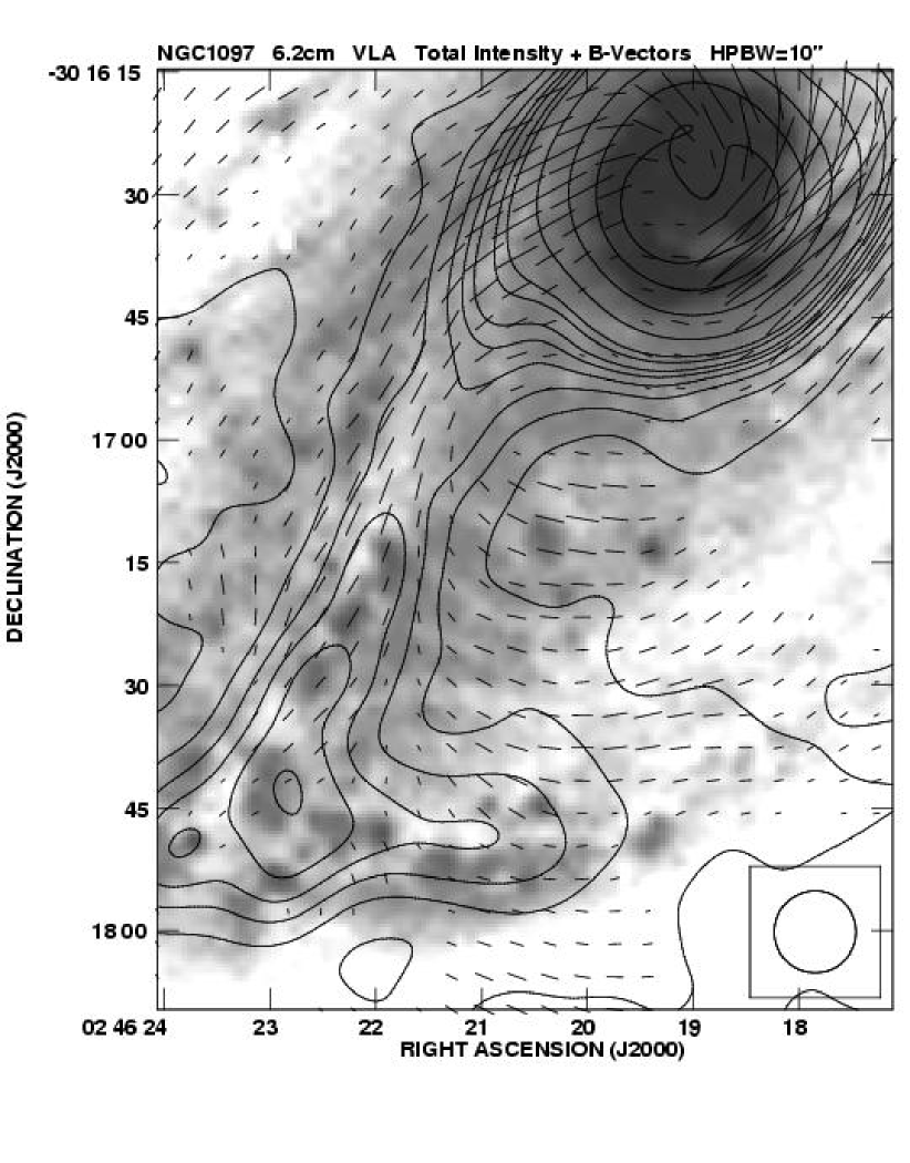
Figure 1: The radio continuum emission in the southern part of NGC 1097, with the galactic centre at top right, observed at $\lambda 6.2\,{\rm cm}$ with the VLA (see Paper III for details). Contours give the total intensity (representing the total magnetic field), dashes show the observed polarization plane rotated by $90^{\circ}$ (representing the regular magnetic field uncorrected for Faraday rotation). The Faraday rotation is about $\pm 20^{\circ}$ at this wavelength (although it can be larger in localized regions). The length of the dashes is proportional to the polarized intensity. The half-power width of the synthesized beam (shown in the lower right corner) is 10″. The background optical B-band image (grey scale) was obtained at the Cerro Tololo Interamerican Observatory by H. Arp. The bar major axis is at an angle $-30^{\circ}$ and the disc major axis (the line of nodes) is at $-45^{\circ}$, both with respect to the south-north direction. The south-western side of the galaxy is closer to us.

Moreover, the polarization intensity (a measure of the strength of the regular magnetic field) in NGC 1097 has a broad local maximum upstream of the dust lanes, where gas density has deep minimum. The regular magnetic field shows hardly any enhancement in the dust lanes. It is also surprising that the regular magnetic field does not show any discontinuity associated with the shock. The sharp turn in magnetic lines leading to a depolarized strip detected by Beck et al. (1999) has been resolved in later observations (Beck et al. 2001b, Paper III) into a smooth turning of the magnetic lines in the region 1 kpc upstream of the dust lanes (Fig. 1). The turn is even smoother in NGC 1365 and occurs about 3 kpc upstream of the compression region (Paper III). Thus, there is no clear signature of any shock-related compression or sharp deflection in the regular magnetic field. It appears that shock effects in the magnetic field may have been mostly eradicated by the enhanced turbulent diffusion in the sheared shock region. The verification and quantification of this effect is one of the main goals of this paper.

There are thin, feather-like, dust filaments bent in a similar way upstream of the main dust lane, seen in the optical photographs of NGC 1097 and NGC 1365. The observed magnetic field is well aligned with these filaments, especially at a distance of 1–3 kpc upstream of the shock front in NGC 1097 (see Fig. 1). Similar filaments have been observed in NGC 5383 by Sheth et al. (2000) who observe that they are associated with H ii regions and propose that the high density and low shear in the filaments make them hosts to star forming regions. If the dust filaments trace the streamlines, the velocity vectors must deviate from the streamlines predicted for this region by gas dynamical simulations (see e.g. Fig. 12 in Roberts et al. 1979, Fig. 2b in A92, and Figs 16 and 26 in Lindblad et al. 1996 where the streamlines have sharp cusp rather than turn smoothly upstream of the shock front). If the magnetic field is sufficiently strong in that region it may control the shape of the dust filaments; however, the occurrence of a dynamically dominant magnetic field has to be confirmed observationally and then explained.

These facts imply that the physics involved is more complicated than that of a simple shock with passive magnetic field. The equipartition strength (with respect to the cosmic rays) of the observed regular magnetic field is about $7\,\mu{\rm G}$ upstream of the dust lane in the southern part of NGC 1097 (Beck et al. 1999). Taking a gas number density of $n=0.1$–$0.2\,{\rm cm^{-3}}$ (from A92), we obtain an Alfvén speed of 30–$50\,{\rm km\,s^{-1}}$. This is much larger than the speed of sound (and, presumably, the turbulent velocity if it has the standard value of $10\,{\rm km\,s^{-1}}$) and is comparable to the shearing velocity in most of the bar region. Hence the magnetic energy density seems to be comparable to the kinetic energy density in the regular shearing motion and much exceeds the thermal energy density. It follows that a fully consistent model of gas flow in barred galaxies should include magnetic fields, a factor systematically neglected in all gas dynamical models of barred galaxies. In this paper we discuss models of regular magnetic field evolution in the velocity field resulting from Athanassoula’s (1992) gas dynamical model in order to assess the extent of the problem, i.e. to establish which features of the observed magnetic field can be readily explained by existing knowledge of the gas flow in barred galaxies and which appear to demand more advanced MHD modelling.

Models of magnetic field evolution in barred galaxies, without the inclusion of dynamo action, have been considered by Otmianowska-Mazur et al. (1997), who used a velocity field resulting from $N$-body simulations (with 38,000 stars and 19,000 molecular clouds). As usual with $N$-body simulations with a modest number of particles, their density distribution has only a moderate enhancement near the bar major axis where dust lanes occur in real galaxies. The simulated magnetic field concentrates in the spiral arms outside the bar region and is weak in the bar. Since the magnetic field is not supported by any dynamo action, it decays in less than $5\times 10^{8}\,{\rm yr}$.

Dynamo models for barred galaxies have been considered by Moss et al. (1998, 1999) who used the gas velocity field obtained from $N$-body simulations with 200,000 stars and 40,000 gas particles. Their density field shows appropriately stronger density contrasts and the inclusion of dynamo action results in persistent magnetic structures. However, the distribution of particles in such models is sparse and uneven, so it is difficult to define reliably a velocity field in low-density regions. This leads to serious complications in magnetic field modelling, and so we prefer to use a velocity field obtained from gas dynamical simulations.

Our model focuses on the regular magnetic field, and the effects of interstellar turbulence on the magnetic field are parameterized in terms of turbulent transport coefficients, including a standard $\alpha$-effect (Moffatt 1978, Parker 1979, Krause & Rädler 1980). The formulation would be similar for alternative mechanisms, such as a magnetic buoyancy driven dynamo, as suggested by Moss et al. (1999b). The key feature of our model is the inclusion of a realistic representation at high spatial resolution of the velocity field in barred galaxies.

We also report briefly in Sect. 4.5 on our discovery of a rather remarkable dynamo effect in galactic discs with positive dynamo number, where the dynamo is driven by noncircular motions rather than by differential rotation. This may be of interest in the wider context of dynamo theory.

2 The alignment of magnetic and velocity fields

As noted by Beck et al. (1999), the regular magnetic field in the bar region of NGC 1097 seems to be aligned with the velocity field of A92, especially in regions with stronger velocity shear. This can be seen from a comparison of Fig. 1, where we present the polarization map of NGC 1097, with the magnetic field orientation indicated with dashes, and Fig. 2 where a velocity field from A92 is shown. Such an alignment is not typical of normal spiral galaxies where magnetic field lines are inclined to the streamlines by $10^{\circ}$–$30^{\circ}$, presumably due to the dynamo action (e.g., Beck et al. 1996, Beck 2000, Shukurov 2000). In the presence of a strongly sheared velocity, the local structure of the magnetic field will be controlled by the local velocity shear. In barred galaxies, the shear of the noncircular velocity field is strong enough to make the form of their magnetic fields markedly different from those found in normal spiral galaxies.

Ignoring the effects of dynamo action, the large-scale field will be frozen into the flow in regions with $R_{\rm m}=uL/\eta\ga 1$, where $u\simeq 100\,{\rm km\,s^{-1}}$ is the regular shearing velocity, $L\simeq 3\,\,{\rm kpc}$ is its scale in the bar region, and $R_{\rm m}$ is the magnetic Reynolds number based on the turbulent magnetic diffusivity $\eta$. Thus, the field will be aligned with the flow if $\eta\la 10^{29}\,{\rm cm}^{2}\,{\rm s}^{-1}$.

However, the alignment of magnetic field and the flow can be affected by dynamo action even at large values of $R_{\rm m}$. Dynamo action is needed to maintain the global magnetic field against the effects of winding by differential rotation and tangling by turbulence, which would lead eventually to enhanced Ohmic decay. Therefore, we also require that the dynamo is unable to misalign the field and the streamlines: the local growth rate of the magnetic field $\gamma$ must be smaller than the shear rate, i.e. $\gamma\la u/L$ with $\gamma\simeq D^{1/2}\eta/h^{2}$, where $D=\alpha uh^{3}/(L\eta^{2})$ is the local dynamo number and $\alpha$ is the alpha-coefficient. This yields $\alpha L/uh\la 1$, or $Lv_{\rm t}/hu\la 1$, where $v_{\rm t}$ is the turbulent velocity and $\alpha\leq v_{\rm t}$ (since $\alpha$ cannot exceed the turbulent speed – see, e.g., Sect. V.4 in Ruzmaikin et al. 1988). In normal galaxies where $u$ is dominated by the streaming velocity produced by the spiral pattern and so $L/h\simeq 2$–3 and $v_{\rm t}/u\simeq 1$, this inequality is not satisfied and we can not expect strong alignment between the streamlines and magnetic lines. Indeed, the magnetic pitch angle (i.e. the angle between the regular magnetic field and the streamlines) is about 1/3 radian, plausibly consistent with this estimate. On the other hand, the shear rate $u/L$ is significantly larger in barred galaxies and we can expect a much closer alignment in the regions where $L\la 3\,{\rm kpc}$ and $u\ga 60\,{\rm km\,s^{-1}}$, where the above inequality is satisfied. In other words, we expect that barred galaxies contain large regions where dynamo action is overwhelmed by the local velocity shear resulting in a tight alignment of the magnetic field with the shearing velocity (more precisely, with the principal axis of the rate of strain tensor). On the other hand, there may be regions of enhanced diffusivity and/or reduced shear where the alignment is reduced (see Fig. 7).

The velocity field, but not the magnetic field, looks different in the inertial and corotating frames. We can expect a rather close general alignment between $\@vec{B}$ and $\@vec{u}$ in the reference frame corotating with the bar for the following reason. Nonaxisymmetric magnetic field patterns must rotate rigidly to avoid winding up by differential rotation (and it is the dynamo which can maintain such fields). With a nonaxisymmetric perturbation from the bar (or spiral arms), the magnetic modes that are corotating with the perturbation will be preferentially excited (e.g. Mestel & Subramanian 1991; Moss 1996, 1998; Rohde et al. 1999). Thus, the regular magnetic field will corotate (or nearly corotate) with the bar, and this is a physically distinguished reference frame. (All magnetic field configurations discussed in this paper, except those in Sect. 4.5, do exactly corotate with the bar.) So, an approximate alignment between $\@vec{B}$ and $\@vec{u}$ is expected in the corotating, but not in the inertial, frame.

3 The model

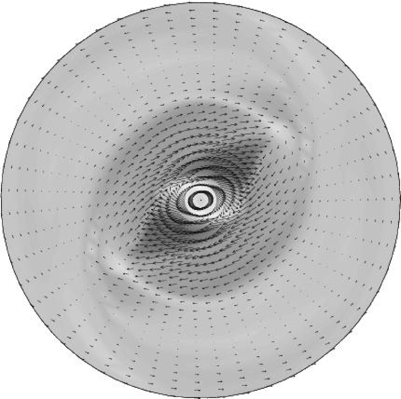
Figure 2: The velocity and gas density (grey scale, lighter shades correspond to higher values) fields in the frame corotating with the bar, from Model 001 of A92. The sense of rotation is clockwise. The bar major axis is at an angle of $45^{\circ}$ to the vertical, the frame radius is $8\,{\rm kpc}$ and the corotation radius is $r_{\rm c}\approx 6\,{\rm kpc}$.

3.1 The gas velocity field

The velocity field was taken from data supplied by E. Athanassoula, corresponding to Model 001 shown in Fig. 2 of A92. This model is two-dimensional, with $\@vec{u}=(u_{x}(x,y),u_{y}(x,y),0)$ in cartesian coordinates $(x,y,z)$. The gas velocity and density fields are steady in the frame rotating with the bar (the corotating frame). The stellar bar extends approximately between the ends of the dust lanes (shown as a light shade in Fig. 2). We reproduce in Fig. 2 the velocity field in this frame rotating in a clockwise sense with angular velocity of about $34\,{\rm km\,s^{-1}}\,{\rm kpc}^{-1}$, placing the corotation radius at about $r=r_{\rm c}\approx 6\,{\rm kpc}$. The streaming velocities relative to the rotating frame are as large as $100\,{\rm km\,s^{-1}}$ near the shock fronts, which are slightly offset from the major axis of the bar. Regions where the sheared velocity is comparable with the rotational velocity are widespread in the bar region. A shock near the dust lanes is just resolved in the data. The region in which the velocities are available is $16\,{\rm kpc}$ across.

The magnetic fields obtained using this velocity field will be compared with observations of NGC 1097 where the corotation radius is $r_{\rm c}\approx 12\,{\rm kpc}$ (assuming a distance to NGC 1097 of 17 Mpc); the length scales are therefore renormalized correspondingly before any comparison is made. However, when discussing the computational results in Sects. 4 and 4.5 we retain the original length scale of A92 with corotation at $6\,{\rm kpc}$. Since the model of A92 refers to a generic barred galaxy rather than to the galaxy NGC 1097 specifically, our comparison with observations can only be qualitative.

3.2 The dynamo model

The basic dynamo model, as applied to galaxies with strong noncircular motions, is described in Moss et al. (1999); it uses the ‘no-$z$’ approximation (Moss 1995), replacing derivatives perpendicular to the galactic midplane ($z$-direction) with inverse powers of $h$, the disc semi-thickness. This is in some ways consistent with the two-dimensional flow model of A92. The mean field dynamo equations are solved for the magnetic field components in the directions orthogonal to $z$. ($B_{z}$ is given in principle by the condition $\nabla\cdot\@vec{B}=\@vec{0}$.) The resulting magnetic field can be thought of as an approximation to the field in the mid-plane, or to represent values averaged vertically over the disc.

We made one significant amendment to the model. Phillips (2001) has showed that the dynamo growth rates in the ‘no-$z$’ model can be made to agree more closely with those of the asymptotic analysis (e.g. Ruzmaikin et al. 1988) by including a correction factor of $\pi^{2}/4$ into the terms representing diffusion in the vertical direction, and so we also included these factors. Thus the local marginal dynamo numbers for our models can now be expected to be fairly directly comparable to standard values of about 10.

The large velocity shear present in barred galaxies resulted in unsatisfactory numerical behaviour of the numerical algorithm previously employed (e.g. Moss et al. 1998, 1999; Moss 1995), and so a new version in cartesian coordinates was written, using a second order Runge–Kutta method for time-stepping, and second-order accurate space discretisation. This code solves the ‘no-$z$’ dynamo equations in the frame corotating with the bar. The earlier calculations were carried out using the $\alpha\omega$ formulation, but now we allow for the regeneration of both meridional and azimuthal regular magnetic field by interstellar turbulence (the $\alpha^{2}\omega$ dynamo). The dynamo equation has the form

$$\frac{\partial\@vec{B}}{\partial t}=\nabla\!\times\!(\@vec{u}\times\@vec{B}-{\textstyle\frac{1}{2}}\nabla\eta\times\@vec{B}+\alpha\@vec{B})-\nabla\!\times(\eta\nabla\!\times\!\@vec{B}),$$ (1)

where $\@vec{u}$ is the regular velocity field described in Sect. 3.1, $\alpha$ parameterizes the dynamo action of the interstellar turbulence, and $\eta$ is the turbulent magnetic diffusivity (see, e.g., Ruzmaikin et al. 1988, Beck et al. 1996). In Eq. (1), we ignore any vertical ($z$-wise) variation of $\eta$, but allow a variation in the disc plane. (In principle we might, in the spirit of the no-$z$ approximation, have approximated the effects of a halo diffusivity larger than that in the disc by an estimate of the form $\partial\eta/\partial z\sim\eta(x,y)/h$.) The equation is solved in a cylindrical region with radius $8\,{\rm kpc}$. We allow for nonlinear dynamo effects leading to the saturation of the magnetic field growth by adopting

$$\alpha=\alpha_{0}\frac{\tilde{\alpha}(\@vec{r})}{1+\xi\@vec{B}^{2}/4\pi\rho(\@vec{r})v_{\rm t}^{2}}\;,$$ (2)

where $\alpha_{0}$ (a typical amplitude of $\alpha$) is a constant, $\tilde{\alpha}(\@vec{r})$ is the normalized background value, and $\rho$ and $v_{\rm t}$ are the gas density and turbulent velocity. We are thus assuming that the large-scale magnetic field significantly reduces the $\alpha$-effect when its energy density approaches that of the turbulence; $\xi$ is a constant, introduced to suggest some of the uncertainty about the details of this feedback. When estimating field strength from our models we set $\xi=1$, but this fundamental uncertainty should be kept in mind. (Indeed, it is quite possible that, rather than being a constant, $\xi$ could depend on local conditions.) We assume that $v_{\rm t}=10\,{\rm km\,s^{-1}}$, and $\rho$ is taken from the same gas dynamical model of A92 as the velocity field $\@vec{u}$. It is often assumed that $\alpha\propto\omega$ with $\omega$ the angular velocity of rotation. We first consider models with $\alpha$ constant apart from quenching effects, i.e. $\widetilde{\alpha}(\@vec{r})=1$, and then put $\widetilde{\alpha}(\@vec{r})=\omega(r)/\omega(r_{\omega})$, where we arbitrarily choose $r_{\omega}=0.3R$, and $R=8\,{\rm kpc}$. (Note that $\omega(r_{\omega})/\Omega_{0}\approx 0.22$ where the unit angular velocity $\Omega_{0}$ is introduced in Sect. 3.3.) We choose this normalization so as to have the dimensionless quantities of order unity in the outer parts of the galaxy.

We can estimate the $z$-averaged vertical field in the disc, by using the condition $\nabla\cdot\@vec{B}=0$, and estimating $\partial B_{z}/\partial z$ by $B_{z}/h$. This vertical magnetic field (not shown in Fig. 4 and other similar figures), is small on average, being about 10 times weaker than the average horizontal field. However, the vertical field is significant in regions with pronounced structure in the horizontal field (e.g. the shock front and the central region) where it can be comparable to the horizontal field.

Note that the dynamo equations with the quadratic nonlinearity (2) allow the transformation $\@vec{B}\to-\@vec{B}$; therefore the magnetic field vectors in the figures shown below can be reversed.

Equation (1) is nondimensionalized in terms of length $R$, the characteristic disc radius, and the magnetic diffusion time across the galactic disc, $h^{2}/\eta_{0}$ with $h$ the disc scale height and $\eta_{0}$ a typical value of $\eta$. Magnetic field is measured in units of $B_{0}=\sqrt{4\pi\rho_{0}v_{\rm t}^{2}/\xi}$ (corresponding to equipartition between the turbulent and magnetic energies), where $\rho_{0}$ is the maximum density. The induction effects arising from turbulence and large-scale motions are quantified by dimensionless dynamo numbers

$$R_{\alpha}=\frac{\alpha_{0}h}{\eta_{0}}\;,\quad R_{\omega}=\frac{\Omega_{0}h^{2}}{\eta_{0}}\;,$$

where subscript zero denotes a characteristic value of the corresponding variable. From here onwards we refer only to dimensionless quantities, unless explicitly stated otherwise.

Although we are studying an $\alpha^{2}\omega$ dynamo characterized by two separate dimensionless parameters $R_{\alpha}$ and $R_{\omega}$, it is still useful to consider the dynamo number $D=-R_{\alpha}R_{\omega}$ as a crude measure of the dynamo intensity. $R_{\omega}$ is positive here because it is defined in terms of a typical angular velocity $\Omega_{0}>0$. In the standard asymptotic analysis for galactic dynamos (see Sect. VI.4 in Ruzmaikin et al. 1988), $D$ is defined in terms of $rd\omega/dr$, which is negative. Thus we have introduced a minus sign into our definition of $D$ so that, consistent with Ruzmaikin et al., the standard galactic dynamo has $D<0$. Our results are primarily a function of $D$ (for given $f_{\alpha}$, $f_{\eta}$, see Eq. (5)) being quite insensitive to the relative values of $R_{\alpha}$ and $R_{\omega}$ in the parameter range considered; this indicates that rotational velocity shear dominates in the production of the azimuthal magnetic field (i.e. we have approximately an $\alpha\omega$ dynamo). The dynamo can maintain the regular magnetic field if $|D|\geq D_{{\rm cr}}$, where $D_{{\rm cr}}$ is a critical dynamo number, which depends weakly on details of the model (Sect. VI.4 in Ruzmaikin et al. 1988); as a rough estimate, $D_{{\rm cr}}\simeq 8$ in the simple model discussed in Sect. 4.1. This marginal value (obtained with the velocity field of A92) is close to that found for a calculation using only the axisymmetric part of the azimuthal velocities.

The computational domain formally is $-1\leq x,y\leq+1$, but we solve only in the region $r=(x^{2}+y^{2})^{1/2}\leq 1$, with boundary conditions $B_{x},B_{y}=0$ at $r=1$. Field amplitudes are found to be small near the boundaries of the domain in most cases considered, and so the boundary conditions remain self-consistent throughout the simulations. The region $r>1$ is ignored; formally $\@vec{B}=0$ there. Our choice is conservative, being arguably the least favourable for dynamo action; for example dynamo action occurring outside $r=8\,{\rm kpc}$ could feed field into the region, interior to this radius, where the equations are solved.

Our standard computational grid has $160$ mesh lines in both the $x$- and $y$-directions, uniformly distributed over $-1\leq x,y\leq 1$; we made a trial integration on a finer grid, finding insignificant differences in our results.

3.3 Units

We choose the size of the formal computational domain to be 16 kpc, consistent with that of A92. Thus $R=8\,{\rm kpc}$, and we choose $h=0.4\,{\rm kpc}$, although the overall nature of the solutions is relatively insensitive to the latter choice: $h$ appears in the dimensionless control parameters $R_{\alpha}$ and $R_{\omega}$, and the overall field strength depends on their product $D$. With $\Omega_{0}=150\,{\rm km\,s^{-1}}\,{\rm kpc}^{-1}$ (of order the value in the inner $1\,{\rm kpc}$ radius), we have $R_{\omega}\approx 72/\eta_{26}$, where $\eta_{26}=\eta_{0}/10^{26}\,{\rm cm}^{2}\,{\rm s}^{-1}$ and, if $\alpha_{0}$ is a few km s^-1, then $R_{\alpha}$ will be of order unity. We assume that $v_{t}=10\,{\rm km\,s^{-1}}$ everywhere, so that, with $\rho_{0}\approx 3.5\times 10^{-24}\,{\rm g}\,{\rm cm^{-3}}$, the unit magnetic field strength is $B_{0}=6.6\times 10^{-6}\xi^{-1/2}\,{\rm G}$.

Neither $v_{\rm t}$ nor $c_{\rm s}$ are well known from observations of barred galaxies. However, Englmaier & Gerhard (1997) found that sound speeds less than about $20\,{\rm km\,s^{-1}}$ are necessary to produce shocks shifted away from the bar axis. We note in this connection that random velocities of molecular clouds in the central regions of NGC 1097 are as high as $35\,{\rm km\,s^{-1}}$ (Gerin et al. 1988), i.e. 3–4 times larger than the turbulent velocities at larger distances from the centre. A similar central enhancement in the velocity dispersion of molecular gas has been detected in NGC 3504 (Kenney et al. 1993). We take $v_{\rm t}=10\,{\rm km\,s^{-1}}$ as a uniform background value, but the turbulent intensity is assumed to be enhanced in the shock fronts and in the central region as described in Sect. 3.4.

A representative value of the turbulent magnetic diffusivity is $\eta_{0}\simeq\frac{1}{3}v_{\rm t}l\simeq 10^{26}\,{\rm cm}^{2}\,{\rm s}^{-1}$ for $v_{\rm t}=10\,{\rm km\,s^{-1}}$, where $l\simeq 100$ pc is the turbulent scale. A convenient estimate of $\alpha$ is (Sect. V.4 in Ruzmaikin et al. 1988)

$$\alpha \simeq \min{\left(\displaystyle\frac{l^{2}\Omega}{h},v_{\rm t}\right)}$$ (3)

$$= \min{\left[0.5\,{\rm km\,s^{-1}}\,\left(\displaystyle\frac{\Omega}{20\,{\rm km\,s^{-1}}\,{\rm kpc}^{-1}}\right),10\,{\rm km\,s^{-1}}\right]},$$ (4)

where we neglect possible local enhancements of turbulent velocity beyond $10\,{\rm km\,s^{-1}}$. With the above values of $l$, $h$ and $\Omega_{0}$, we obtain $\alpha_{0}\simeq 4\,{\rm km\,s^{-1}}$. Thus, our representative values of the dynamo coefficients are $R_{\alpha}=5$ and $R_{\omega}=70$. Since Eq. (3) is just an order of magnitude estimate, we consider that a variation of a factor 3 in the dynamo coefficients is quite acceptable.

3.4 Enhancement of turbulence by shear

Figure 3: Contours of $\eta/\eta_{0}-1$ with $f_{\eta}=3$ in Eq. (5) with $\@vec{u}$ from A92, as used in Sect. 4.2. The 5 contour levels are equally spaced with a range from 0.10 to 0.90. As in Fig. 2, the frame radius is 1.7 times the corotation radius.

We allow for the possibility that both $\eta$ and $\alpha$ may be enhanced where shear flow instabilities are likely to occur, by writing

$$\alpha=\alpha_{0}\left(1+f_{\alpha}\frac{S}{S_{\rm max}}\right),\quad\eta=\eta_{0}(\@vec{r})\left(1+f_{\eta}\frac{S}{S_{\rm max}}\right),$$ (5)

where $f_{\alpha}$ and $f_{\eta}$ are constants and $S=|\partial u_{x}/\partial y|+|\partial u_{y}/\partial x|$, ${\mbox{\boldmath$u$}}=(u_{x},u_{y})$ and $S_{\rm max}$ is the maximum value of $S$. For given values of $R_{\alpha}$, $R_{\omega}$ and/or $D$, the local dynamo action is weakened if $f_{\eta}>0$, and enhanced if $f_{\alpha}>0$. Contours of $\eta/\eta_{0}-1$ with $f_{\eta}=3$ are shown in Fig. 3; our models have magnetic diffusivity enhanced in the dust lanes and in the innermost 1–2 kpc.

The effects of varying $\alpha$ and $\eta$ cannot be disentangled completely since it is the ratio $\alpha/\eta^{2}$ that affects magnetic fields generated by an $\alpha\omega$ dynamo. Therefore, the result of enhanced $\alpha$ can be reproduced, quite closely, by reducing $\eta$ instead. Thus, in order to keep the models as simple as possible, we preferred to take $f_{\alpha}=0$ in most simulations. Furthermore, with $S$ defined after Eq. (5), the turbulent transport coefficients $\alpha$ and $\eta$ with $f_{\alpha},f_{\eta}\neq 0$ would be enhanced even in rigidly rotating regions. The most important result of this is that $\eta$ can be unrealistically large in the central parts of the disc in models discussed below. A perhaps more physically meaningful prescription could be $S=|\partial u_{x}/\partial y+\omega|+|\partial u_{y}/\partial x-\omega|$. However, the effect of the latter refinement is reduced when working in the rotating frame and, moreover, it would plausibly be similar to that of reducing $f_{\eta}$. So we leave this refinement for future, more advanced models. A trial calculation showed that the effect is small when $f_{\eta}\la 3$ and $\alpha_{0}$ is constant.

We suggest that the enhancement of the turbulent diffusivity in the shear flow (the dust lane) is due to the development of flow instabilities. The enhancement will be sufficient to reduce the contrast in the magnetic field if the turbulent diffusion time is shorter than the advection time across the dust lane width: $d^{2}/\eta<d/c_{\rm s}$ with $d\simeq 0.5\,{\rm kpc}$ in NGC 1097 (Regan et al. 1995, 1997) and we have assumed that the transverse velocity immediately behind the shock is equal to the speed of sound $c_{\rm s}\simeq 10\,{\rm km\,s^{-1}}$ (e.g. Roberts et al. 1979, Englmaier & Gerhard 1997). This yields $\eta>1.5\times 10^{27}\,{\rm cm}^{2}\,{\rm s}^{-1}$ for the turbulent magnetic diffusivity within the dust lanes, so $\eta$ would have to be increased about tenfold from the background value $\eta_{0}$, in order to reduce the field contrast.

The Kelvin–Helmholtz instability is an obvious candidate for turbulence amplification in the dust lanes (see Townsend (1976 ) or Terry (2000) for a recent discussion of turbulence in shear flows and Ryu et al. (2000) and Brüggen & Hillebrandt (2001) for a discussion of mixing enhancement by the instability). The growth rate of the instability in a piecewise continuous flow is given by

$$\gamma_{\rm KH}=\frac{U}{2d}K\left[2K^{-1}-1-2K^{-2}\frac{\sinh{K}}{\exp{K}}\right]^{1/2},$$

where $K=kd$ with $k$ the wavenumber in the direction of the shear flow, $d\simeq 0.5\,{\rm kpc}$ is the transverse width of the sheared region and $U\simeq 100$ kms^-1 is the velocity difference across it. The growth rate has a maximum, $\gamma_{\rm max}\approx 0.1U/d$, for $K\approx 0.8$. The resulting enhancement in the turbulent velocity can be estimated as $v_{\rm t}\simeq v_{\rm t0}\exp(\gamma_{\rm max}d/c_{\rm s})$, where $v_{\rm t0}\simeq c_{\rm s}\simeq 10\,{\rm km\,s^{-1}}$ is the turbulent velocity upstream of the dust lane, and we have assumed that the transverse velocity immediately after the shock is equal to the speed of sound, so the residence time of the matter in the unstable region is given by $d/c_{\rm s}$. This yields $\gamma_{\rm max}d/c_{\rm s}\simeq 1$, so the turbulent velocity in the dust lane is expected to be 2–3 times larger than the upstream value of $10\,{\rm km\,s^{-1}}$. The most unstable mode has a scale of $l=2\pi d/0.8\approx 4\,{\rm kpc}$. The resulting enhancement in the turbulent diffusivity $\eta\simeq\frac{1}{3}v_{\rm t}l$ can be as large as by a factor of 100, but this enhancement will be limited by the fact that only a part of the flow produced by the instability will be randomized, and simultaneously the effective value of $l$ will be reduced. Arguably, a better estimate of $\eta$ resulting from the instability is $\eta\simeq\frac{1}{3}v_{\rm t}^{2}\gamma_{\rm max}^{-1}\simeq 3v_{\rm t0}d\simeq 15v_{\rm t0}l$, implying enhancement by a factor of 50. The above estimates are upper limits, referring to the maximum rather than the mean enhancement. The enhancement of $\eta$ used in our models ranges up to a factor of $f_{\eta}+1=6$, and the case $f_{\eta}=3$ is illustrated in Fig. 3.

A magnetic field parallel to the shear velocity can suppress the Kelvin–Helmholtz instability if $V_{\rm A}>U$ (Chandrasekhar 1981), but this inequality is not satisfied in our case.

Apart from the Kelvin–Helmholtz instablity, enhanced small-scale three-dimensional motions can arise from local perturbations to the gravitational field as discussed by Otmianowska-Mazur et al. (2001).

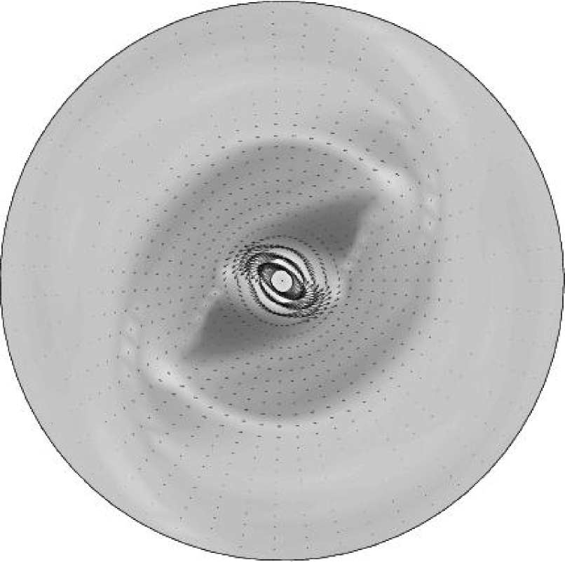
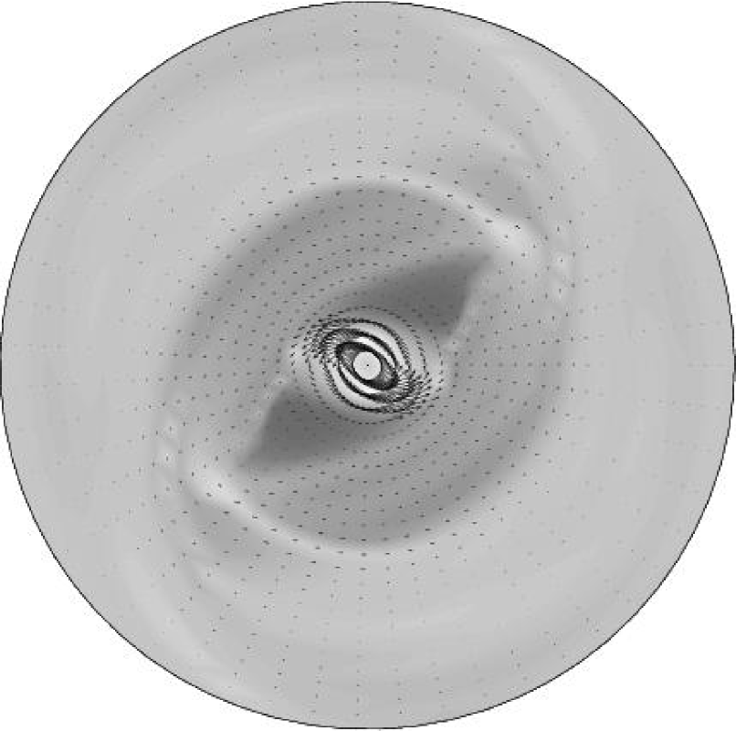
 (a)
 (b)

Figure 4: Vectors of the horizontal magnetic field for the model with $R_{\alpha}=0.3$, $R_{\omega}=36$, $f_{\alpha}=f_{\eta}=0$. The circumscribing circle has radius 8 kpc. Shades of grey show gas density, with lighter shades corresponding to higher values. The magnetic field vectors have been rescaled by $\@vec{B}\to\@vec{B}/B^{n}$ with $n=0.3$, to improve the visibility of the field vectors in regions with small $B$. Panel (a) shows the field vectors over the entire computational domain, whereas in (b) the inner region has been omitted, in order to show the structure in the outer regions of the disc.

4 Results

4.1 Our basic model

We first examined the simplest dynamo model with $\widetilde{\alpha}(\@vec{r})=1$, $f_{\alpha}=f_{\eta}=0$, i.e. $\eta$ is constant, unmodified by the shear, and $\alpha$ is a function only of the magnetic field and gas density, via the $\alpha$-quenching. We experimented with several parameter combinations, and first discuss here a model with $\eta_{0}=2\times 10^{26}\,{\rm cm}^{2}\,{\rm s}^{-1}$ so $R_{\omega}=36$. With $R_{\alpha}=0.3$ (giving $D=-10.8$), the dynamo is slightly supercritical in the central parts of the galaxy ($r<1$–2 kpc) and subcritical at larger radii. The eventual magnetic field configuration is steady in the corotating frame, and its structure is shown in Fig. 4, superimposed on the gas density. Here, and in the other figures, we have smoothed the magnetic field over a scale of about 0.6 kpc, to approximate the resolution of the observations. For comparison, the radio observations have a beamwidth of $10\arcsec$ ($0.8\,{\rm kpc}$) for NGC1097 and $15\arcsec$ (2 kpc) for NGC 1365. We see that the magnetic field is strongly concentrated to the central regions ($r\la 2\,{\rm kpc}$ in this model with uniform diffusivity, reflecting the strong dynamo action in this region where the angular velocity and its shear are maximal. This feature remains even when the dynamo number is very substantially increased. In this model, the maximum field strength of about $0.5B_{0}$ is reached at $r\approx 0.7\,{\rm kpc}$ (corresponding to about $3\,\mu{\rm G}$); the field is negligible beyond $r\simeq 2\,{\rm kpc}$. Observations of NGC 1097 suggest that the ratio of the regular field strength in the inner region ($r/r_{\rm c}\simeq 0.1$) to that in the outer bar region is about 2, and so this model is unsatisfactory. Note that this feature is little altered by the smoothing to the resolution of the observations.

Even when $|D|$ is increased by an order of magnitude, the model magnetic field remains strongly concentrated to the central regions. Note that in all our models the field strength increases with $|D|$, but in order to obtain field strengths comparable with those observed near to the corotation radius, it is necessary to increase $|D|$ to values at the margin of what is plausible, and the field in the inner regions is then significantly larger than observed. The overall field structure is relatively insensitive to the magnitude of $D$. An obvious problem with this basic model with $\eta=\mbox{const}$ is that it yields an unrealistically weak magnetic field in the outer regions and perhaps a too strong contrast in $B$ between the dust lane regions and those upstream of them. Thus we now relax the condition that $\eta$ be constant.

Figure 5: Vectors of the horizontal magnetic field for the models with $\widetilde{\alpha}(\@vec{r})=1$, $f_{\alpha}=0$, $R_{\alpha}=3$, $R_{\omega}=72$. (a) $f_{\eta}=1$, (b) $f_{\eta}=3$, and (c) $f_{\eta}=5$. The circumscribing circle has radius 8 kpc. Shades of grey show gas density, with lighter shades corresponding to higher values. The magnetic field vectors have been rescaled as $\@vec{B}\to\@vec{B}/B^{n}$ with $n=0.3$, to improve the visibility of the field vectors in regions with small $B$.

 (a)  (b)
 (c)

4.2 Models with turbulent diffusivity depending on velocity shear: uniform $\widetilde{\alpha}$

An obvious refinement of the model is to consider the turbulent magnetic diffusivity to be modulated by the shear rate, i.e. to put $f_{\eta}>0$ in Eq. (5), keeping the background value uniform, i.e. $\eta_{0}(\@vec{r})=\mbox{const}$. Note that, as $f_{\eta}$ and thus the magnetic field dissipation increase, so does the marginal dynamo number, for example $D_{{\rm cr}}\approx-27$ when $f_{\eta}=5$, and even $D=-11$ is just subcritical when $f_{\eta}=1$. Also, broadly speaking the effects of taking $f_{\alpha}>0$ for given $R_{\alpha}$ and of increasing $R_{\alpha}$ with $f_{\alpha}=0$ are similar, and so we keep $f_{\alpha}=0$. We now set $\eta_{0}=10^{26}$ cm²s^-1, so that $R_{\omega}=72$ and adopt $R_{\alpha}=3$. Thus the models we discuss now are all substantially supercritical, with the local values of $D$ (calculated from the local values of $\Omega$) of order $-(10^{2}$–$10^{3})$ at $r\la 3\,{\rm kpc}$ and about $-15$ near the corotation radius.

In Fig. 5 we show the field structures for calculations with $f_{\eta}=1,3,5$. Again, the magnetic fields are steady in the rotating frame. Increasing $f_{\eta}$ clearly reduces the dominance of the central field. Also, increasing $\eta_{0}$ to $2\times 10^{26}$ cm²s^-1 ($R_{\omega}=36$) produces little overall effects on the field structure, but does affects the field strength. When, for example, $R_{\omega}=36$, $f_{\eta}=1$, $R_{\alpha}=0.6$ ($D=-22.5$), the maximum field strength is about $0.7B_{0}$; this figure increases to about $6.5B_{0}$ when $R_{\omega}=72$, $f_{\eta}=1$, $R_{\alpha}=3$ ($D=-216$, Fig. 5a) Of this increase, a factor of about 4 can be attributed to enhanced induction by rotational shear which yields $B\simeq B_{0}\left(|D|/D_{{\rm cr}}-1\right)^{1/2}$, and the rest to the noncircular velocities.

A feature of all these solutions is that there is a broad field minimum in the bar region, but with strong magnetic ridges at the positions of the dust lanes and field enhancement in the central part where the circumnuclear ring is observed. This agrees well with the overall distribution of polarized intensity in NGC 1097 and 1365. Nevertheless, the local magnetic energy density near the major axis (upstream of the dust lanes) exceeds the turbulent kinetic energy density. As we discuss in Sect. 5.1, both the model and observed field strengths have a well pronounced structure within the bar region in addition to the ridges elongated with the dust lanes and the central ring.

There is a relatively strong, quasi-azimuthal field upstream of the shock, especially near the ends of the bar. This feature also agrees well with the observations, cf. Fig. 1. For the dynamo parameters of the models illustrated in Fig. 5, the dynamo is locally supercritical nearly everywhere. However, the field structure is rather insensitive to the value of $D$. To illustrate this, we show in Fig. 6 the field vectors with only a slightly supercritical dynamo number ($\eta_{0}=2\times 10^{26}\,{\rm cm}^{2}\,{\rm s}^{-1}$, $R_{\alpha}=0.6$, $R_{\omega}=36$). The field configuration is remarkably similar to that of Fig. 5a, with a much larger dynamo number, except perhaps near the outer boundary. This supports the idea that the field in regions upstream of the dust lanes at larger galactocentric distances is mainly produced not by local dynamo action but rather by advection over almost $180^{\circ}$ from regions at small radii (where the dynamo action is stronger) on the other side of the bar. We note that the half-rotation time of the gas at $r\simeq 5\,{\rm kpc}$ is shorter than magnetic diffusion time $h^{2}/\eta_{0}\simeq 5\times 10^{8}\,{\rm yr}$. If the dynamo is strong enough ($R_{\alpha}\ga 3$ for $R_{\omega}=72$) the advection produces a magnetic configuration where the magnetic energy density exceeds that of the interstellar turbulence in broad regions, including the region upstream of the shock front. The steep rotation curve at small radii and the large local dynamo numbers found there suggest that the dynamo is particularly efficient in the inner region. This field is then transported outwards by the noncircular velocities and further enhanced by shear.

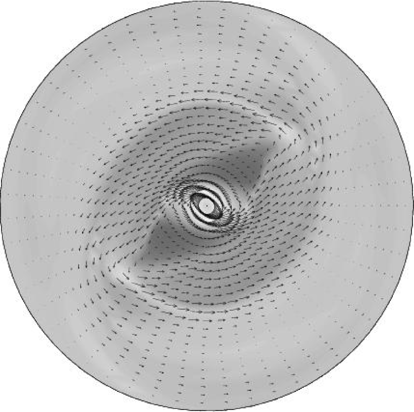
Figure 6: As in Fig. 5a, but for $R_{\alpha}=0.6$, $R_{\omega}=36$, $f_{\eta}=1$, giving weak dynamo action.

Figure 7: The alignment of the regular magnetic and velocity fields in the corotating frame is illustrated with level contours of $\cos\chi=|\@vec{u}\cdot\@vec{B}|/uB$ for the model of Fig. 5a. The levels shown are 0.4 (dotted), 0.7 (dashed) and 0.95 (solid).

Immediately downstream of the shock position, the velocity and magnetic fields are closely aligned. The alignment is fairly good throughout the galactic disc, with the mean angle $\chi$ between magnetic and velocity vectors being about $\chi\approx 20^{\circ}$ ($\langle\cos\chi\rangle\approx 0.93$) in the model of Fig.  5a. As can be seen in Fig. 7, the alignment is especially close outside the bar and slightly reduced within the bar and at the corotation radius. The reduction in the bar can be plausibly attributed to enhanced magnetic diffusivity in the dust lanes and that at corotation to the small local values of $\@vec{u}$ in the rotating frame.

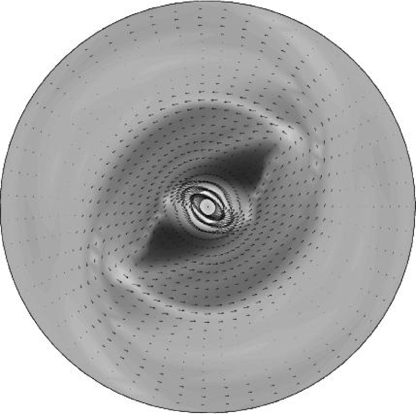
Figure 8: As in Fig. 5a, but for $\widetilde{\alpha}(\@vec{r})\propto\omega(r)$ and $R_{\alpha}=1.5$.

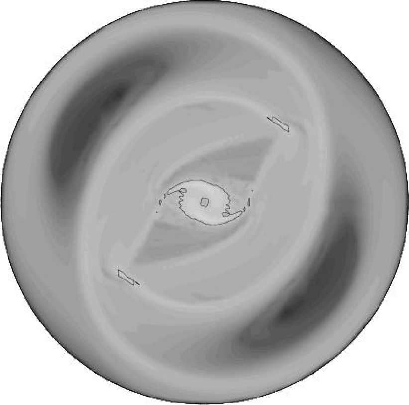
Figure 9: Grey scale map of $B^{2}$ (unsmoothed) for the model shown in Fig. 8. Lighter shades indicate higher values, and the contours shown are for $B^{2}=1$, so the energy density of the regular magnetic field exceeds that of turbulence inside the contours. The circumscribing circle has radius 8 kpc.

4.3 Models with turbulent diffusivity depending on velocity shear: $\widetilde{\alpha}\propto\omega$

We now discuss models in which we set $\widetilde{\alpha}\propto\omega(r)$ (see Sect. 3.2), whilst keeping $f_{\alpha}=0$. Since the dynamo action now becomes more intense in the disc centre, the field strength is more strongly concentrated to the centre for given $f_{\eta}$, than when $\widetilde{\alpha}$ is uniform. As $f_{\eta}$ is varied, these results can be broadly summarized by saying that the field structure is very similar to that when $\widetilde{\alpha}(\@vec{r})$ is uniform, if a larger value of $f_{\eta}$ is now taken. For example, we show in Fig. 8 the field structure when $R_{\omega}=72$, $f_{\eta}=3$, $R_{\alpha}=3$, which can be compared with that shown in Figs. 5a and 5b, with $\widetilde{\alpha}(\@vec{r})=1$ and $f_{\eta}=1,3$ respectively. We note that the effect of setting $\widetilde{\alpha}\propto\omega(r)$ is the opposite of increasing $f_{\eta}$ – the former enhances the central field concentration, the latter decreases it. But the field structure outside of the inner 1–2 kpc is altered only slightly by such changes.

For this model, the maximum field strength is about $3.9B_{0}$, attained at $r/r_{\rm c}\approx 0.1$ (see also Fig. 13). We show in Fig. 9 a grey scale plot of $B^{2}$ for the model of Fig. 8 where magnetic field enhancements in the dust lanes, the spiral arms and the central region are prominent. The field is especially strong in the circumnuclear region and at the ends of the bar. Trailing magnetic arms, emanating approximately from the ends of the bar, are a common feature of the modelled and observed magnetic structures. (This feature is also seen in the model for the weakly barred galaxy IC 4214 of Moss et al. 1999.)

This class of models exhibits the best agreement with observations and we discuss them in detail in Sect. 5.

4.4 Magnetic fields in the absence of dynamo action: the case of pure advection

In this section we attempt to elucidate the roles of the two key ingredients of our model, stretching by the regular velocity and the $\alpha$-effect. In Fig. 10 we show the field structure for a computation with $R_{\omega}=72$, $f_{\eta}=5$, and $R_{\alpha}=0$ (no dynamo action). In the absence of dynamo action this field decays exponentially, with an $e$-folding time of about $10^{8}\,{\rm yr}$. This decay time scale is about 5 times shorter than in normal galaxies because of the enhanced velocity shear that reduces the field scale and so facilitates its decay. Since most barred galaxies in the sample of Paper I do exhibit detectable polarized radio emission and thus possess regular magnetic fields, we conclude that the need for dynamo action in barred galaxies is even stronger than in normal galaxies.

Looking at the spatial structure of the decaying magnetic field, we see that some of the features of the dynamo maintained fields shown in Figs. 5 and 8 are present, particularly the field minimum upstream of the shock, and the trailing magnetic arms outside of the corotation radius. However there is no hint of the relatively strong fields at small radii seen in all models with dynamo action present. In addition, the relative magnetic field strength near the bar major axis is now too low.

Thus it appears that the field structure in the outer regions is relatively insensitive to the parameters of the dynamo model, but that dynamo action is essential to maintain the fields over time scales of gigayears and to produce strong magnetic fields in the region of the circumnuclear ring and upstream of the shock front.

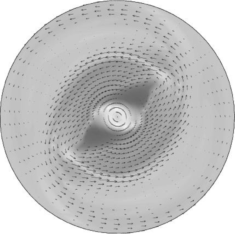
Figure 10: As in Fig. 5, but without any dynamo action: $R_{\alpha}=0$, $R_{\omega}=72$, $f_{\alpha}=0$ and $f_{\eta}=5$. In this case the magnetic field decays on a time scale of about $10^{8}\,{\rm yr}$.

4.5 Results with positive dynamo number

We made some experiments with $R_{\alpha}<0$, i.e. positive dynamo number $D$. This is motivated by suggestions that this may be the case in accretion discs (Brandenburg et al. 1995) even though the origin of turbulence there is quite different from that in galaxies. It is a familiar result for axisymmetric galactic discs that the marginal positive dynamo numbers for dynamo excitation are much larger in magnitude than the marginal values for the usually considered case with $D<0$ – i.e. dynamos with $D>0$ are much harder to excite than those with $D<0$. As mentioned in Sect. 3.2, in the models with $D<0$ the marginal values of $D$ for the models with the full A92 velocity field are essentially unchanged from those found by including only the axisymmetric rotational velocities. When $D>0$, the situation is quite different. A dynamo is excited by the full velocity field at a marginal dynamo number of magnitude considerably less than required to excite the corresponding dynamo driven by the circular motions alone. In other words, when $D>0$ the dynamo is driven by shear due to noncircular velocities rather than from differential rotation.

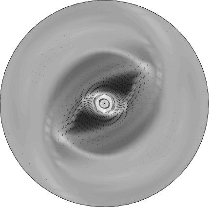
Figure 11: Snapshot of typical vectors of the horizontal magnetic field for the positive dynamo number model with $R_{\alpha}=-6$, $R_{\omega}=36$, $f_{\alpha}=0$, $f_{\eta}=5$, in a format similar to that of Fig. 5.

Figure 12: Profiles of the square of the horizontal magnetic field along cuts perpendicular to the shock front of the model shown in Fig. 8 at (a) 1.5 kpc and (b) 3 kpc galactocentric distance. The total length of each cut is 10 kpc, approximately symmetrical about the position of the shock front, with distance increasing in the upstream direction. The corresponding cuts (with scaled lengths of 20 kpc; $20\arcsec$ corresponds to $r/r_{\rm c}\approx 0.14$) through the map of $\lambda 6$ cm polarized intensity (represented by the vector length of Fig. 1) are shown in (c) and (d) for galactocentric distances of 3 and 6 kpc. The cuts are shown for the same values of $r/r_{\rm c}$ in the model and NGC 1097 and extend over the same linear length.

             (a)                   (b)
             (c)                   (d)

We illustrate our results by discussing a simulation with $R_{\omega}=72$, $f_{\eta}=5$, $f_{\alpha}=0$, $\widetilde{\alpha}(\@vec{r})=1$ and $R_{\alpha}=-6$, a somewhat supercritical value. The magnetic fields are now oscillatory, with a dimensionless period of about 0.48, corresponding to about $1.1\times 10^{8}$ yr. We see in Fig. 11 that the regions of strong magnetic field correspond to the regions of strong velocity shear. The overall field structure varies significantly during the cycle period, and at certain times the amount of structure in the magnetic field is much greater than at others. The magnetic field strength has a maximum in the inner bar region and in two elongated features parallel to the shock fronts. These structures persist through nearly all of the oscillation period. However, the field geometry within the structures changes with time as a magnetic field reversal along a line approximately parallel to the shock front propagates clockwise in Fig. 11. In the lower left-hand part of Fig. 11, weak field directed approximately radially outwards is visible. At a slightly later time, this has grown in strength and this region eats in to the adjacent area of approximately inwardly directed field, strengthening the field reversal. A little later still, the reversal has disappeared, and then the cycle repeats. We emphasize that, for this calculation the field decays when the nonaxisymmetric velocities are removed.

It is clear that these dynamos with positive dynamo numbers generate magnetic fields that are rather different from those observed.

5 Discussion and comparison with observations

5.1 The magnetic field in the shock region

We show in Fig. 12 the variation of $B^{2}$ along two cuts through the shock front region for the model illustrated in Fig. 8, illustrating the variation in the magnetic field strength between the post- and pre-shock regions. Also shown is the observed profile of polarized synchrotron intensity along similarly chosen cuts in NGC 1097. In the case of constant energy density of cosmic-ray electrons, the polarized intensity depends on $B_{\perp}^{2}$, where $B_{\perp}$ is the magnetic field component perpendicular to the line of sight.

Both the model magnetic field and the observed polarized intensity reveal several peaks in $B^{2}$ on each side of the shock front and a pronounced minimum at the shock front itself. The model and observations differ in detail, which is no surprise as inter alia the velocity field and gas distribution used in our models was not designed specifically to fit NGC 1097. We find that the best correspondence between the $B^{2}$ variations from the models and the observed polarized intensity profiles is obtained in models with $\widetilde{\alpha}\propto\omega$ (Sect. 4.3), with $R_{\alpha}\la 1.5$ when $R_{\omega}=72$. Larger values of $|D|$ give weaker peaks near the bar, but taking too small a value of $|D|$ gives rather low field strengths.

Due to the inclination of NGC 1097 ($45^{\circ}$), the difference between $B_{\perp}^{2}$ and $B^{2}$ is typically a factor of 2. Projection effects reduce the polarized intensity upstream of the shock from where magnetic field has significant component parallel to the line of sight, but not in the dust lane where the value of $B_{\perp}$ is closer to that of $B$. This will suppress the amplitude of the secondary peak in polarized intensity in the pre-shock region. With allowance for the unaccounted projection effect, our model shows remarkably good agreement with observations in the number and width of the magnetic peaks in the shock region.

Our models reproduce a smooth turn of the magnetic field vector upstream of the dust lanes observed in NGC 1097 (and also NGC 1365). This turn may be difficult to see in the figures presented here because we have shown magnetic vectors only at a fraction of mesh points. It can be seen from Fig. 7 that the alignment between the magnetic and velocity fields is reduced 1–2 kpc upstream of the shock fronts (dust lanes). Several effects apparently contribute to smear and displace the turn in the magnetic field with respect to that in the velocity field. We argue in Sect. 4.2 that magnetic field can be advected to the pre-shock region from smaller radii (the elongated shape of the streamlines responsible for that can be clearly seen in Fig. 2b of A92, but not that easily in Fig. 2 here). The admixture of magnetic field generated elsewhere must smear any sharp structures produced locally. Furthermore, magnetic field will tend to be aligned with the prinicpal axis of the rate of strain tensor rather than the velocity field itself, and so its turn can start long before it becomes visible in the velocity vectors.

Other effects can be envisaged that might, in principle, result in a smooth turn of magnetic field upstream of the shock fronts. For example, this can be a manifestation of the dynamical influence of the regular magnetic field on the velocity field. However, this is hardly the case in our models where the regular magnetic field does not reach equipartition with even the turbulent kinetic energy in the regions concerned (see Fig. 9). Another possibility is that the turn in the observed field is smoothed by the presence of a magnetic halo with a regular magnetic field smoother than in the disc; however, there is so far no evidence for a polarized halo in NGC 1097. A further option is that the magnetic field is anchored in a warm component of the interstellar medium that has different kinematics than the cold gas (i.e., higher speed of sound); our preliminary analysis of this possibility has given no evidence for this, but we shall return to it elsewhere.

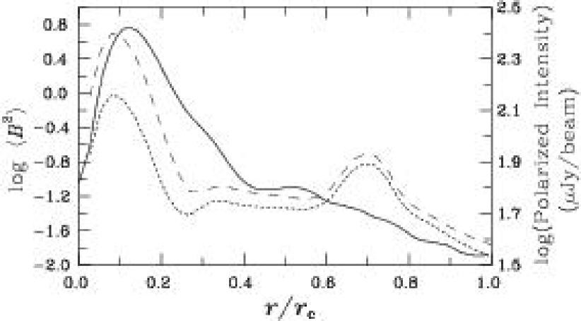
Figure 13: The radial dependence of the azimuthally averaged square of the horizontal magnetic field for the models with $R_{\alpha}=1.5,\ R_{\omega}=72,\ \widetilde{\alpha}\propto\omega$, but with $f_{\eta}=1$ (dashed) and $f_{\eta}=3$ (dotted). For comparison the radial profile of the azimuthally averaged polarized intensity at $\lambda 6\,{\rm cm}$ in NGC 1097 is shown with solid line. Note the logarithmic scale on the vertical axes; $\langle B^{2}\rangle=0$ at $r=0$ in our models.

5.2 Radial profiles of magnetic field

We show in Fig. 13 the dependence of the azimuthally averaged value of $B^{2}$ on radius for the model shown in Fig. 8 and a similar model with larger $f_{\eta}$, and compare it with the observed dependence of polarized intensity on radius. The model reproduces the peak observed close to the centre and has a realistic radial scale. The slower decrease of polarized intensity with galactocentric radius in NGC 1097 can be explained by a steeper rotation curve in the A92 model, which has the turnover radius at $r/r_{\rm c}\approx 0.25$ whereas it occurs at about $r/r_{\rm c}=0.4$ in NGC 1097 (Ondrechen & van der Hulst 1989). The model magnetic field has a pronounced subsidiary peak at $r/r_{\rm c}\approx 0.7$; this peak is related to the strong magnetic arms visible in Fig. 9. A similar peak in the observed radial profile is less pronounced and occurs at a smaller fractional radius.

In our models, the regular magnetic field vanishes on the rotation axis because of its symmetry properties. However, the observed polarized intensity remains significant at $r=0$. We discuss implications of this in the next section.

Table 1: The global magnetic structure in NGC 1097 represented in terms of the amplitudes of the azimuthal Fourier modes ${\cal R}_{m}$, their pitch angles $p_{m}$ and phases $\beta_{m}$ with $m$ the wavenumber. The bottom line shows azimuthally averaged magnetic field strengths obtained assuming ${n_{\rm e}}=0.1\,{\rm cm^{-3}}$ and $h=0.4\,{\rm kpc}$.

		Radial range (kpc)
		2.9–3.7	3.7–4.5	4.5–5.3
${\cal R}_{0}$	$\rm{rad\,m^{-2}}$	$-152$ $\pm 6$	$-141$ $\pm 13$	$-152$ $\pm 17$
$p_{0}$	degrees	$18$ $\pm 1$	$27$ $\pm 2$	$22$ $\pm 2$
${\cal R}_{1}$	$\rm{rad\,m^{-2}}$	$-75$ $\pm 8$	$-88$ $\pm 12$	$-90$ $\pm 10$
$p_{1}$	degrees	$-50$ $\pm 13$	$-71$ $\pm 13$	$-58$ $\pm 7$
$\beta_{1}$	degrees	$-119$ $\pm 6$	$-98$ $\pm 6$	$-122$ $\pm 8$
${\cal R}_{2}$	$\rm{rad\,m^{-2}}$	$110$ ${}^{+3}_{-185}$	$57$ ${}^{+8}_{-145}$	$75$ ${}^{+15}_{-8}$
$p_{2}$	degrees	$0$ ${}^{+1}_{-130}$	$-7$ ${}^{+9}_{-102}$	$-31$ ${}^{+8}_{-91}$
$\beta_{2}$	degrees	$13$ $\pm 4$	$11$ $\pm 15$	$28$ $\pm 8$
$\langle B\rangle$	$\mu\rm{G}$	$5.3$ ${}^{+0.3}_{-1}$	$4.9\,$$\pm 0.6$	$5.3$ ${}^{+0.6}_{-1}$

5.3 The azimuthal structure of the global magnetic field

The azimuthal structure of the regular magnetic field is a useful diagnostic of both the overall structure of the gas velocity and the field generation mechanisms. We have fitted the polarization angles observed in NGC 1097 at $\lambda\lambda 3.5$ and 6.2 cm, for three radial rings between 2.9 and $5.3\,{\rm kpc}$ with a model where the magnetic field is expanded into azimuthal Fourier modes. The model and the fitting procedure are discussed by Berkhuijsen et al. (1997) and Fletcher et al. (2001); Table 1 gives details of the fits. The polarization angles have been obtained from Stokes parameters averaged over $20^{\circ}$ sectors in the $0.8\,{\rm kpc}$ wide rings. The results are presented in terms of ${\cal R}_{m}=0.81\,B_{m}{n_{\rm e}}h$, $p_{m}$ and $\beta_{m}$, where $B_{m}$ (in $\mu$G) is the amplitude of the magnetic mode with azimuthal wave number $m$, ${n_{\rm e}}$ is the thermal electron density in cm^-3, $h$ is the scale height of the thermal ionized layer in pc, $p_{m}$ is the pitch angle of the mode $m$ (i.e. the angle between the field direction and the circumference; $p>0$ indicates a trailing spiral) and $\beta_{m}$ is the azimuthal angle, measured counter-clockwise from the northern end of the major axis of the galaxy, where the mode $m$ ($m\neq 0$) has maximum strength. ${\cal R}_{m}$ is related to the Faraday rotation measure; ${\cal R}_{m}=100\,{\rm rad\,m^{-2}}$ corresponds to a field strength of about $3\,\mu{\rm G}$ for $n_{\rm e}=0.1\,{\rm cm^{-3}}$ and $h=400$ pc. Note that the limited azimuthal resolution of the fits $(m\leq 2)$ does not allow the fitting of the sharp deflection of the $B$ vectors in the shock wave region (Fig. 1).

The amplitudes of the three lowest azimuthal Fourier modes in the observed regular field of NGC 1097 have ratios $1:1:0.5$. The corresponding values for the models shown in Figs. 5a,b,c and Fig. 8 are all $1:0:0.5$. The axisymmetric mode is dominant in both the observed field and in all these models. The relative amplitude of the $m=2$ mode for these models is also in agreement with the observations, having about half the amplitude of the $m=0$ mode.

The magnetic fields in our models do not contain the $m=1$ magnetic mode present in the observed field. This is due to the strict symmetry of the model velocity field (it does not contain any modes with odd $m$) and the inability of the dynamo to maintain the $m=1$ mode on its own. The only mode actively maintained by the dynamo in our models is the axisymmetric one, $m=0$, and the $m=2$ mode arises via distortion of the basic field by a flow with a strong $m=2$ component. In turn, other magnetic modes with $m$ even are also maintained. In real galaxies such a high degree of symmetry of the velocities cannot be expected, and thus a wider range of azimuthal modes will be present in the magnetic field. We note that NGC 1097 is perturbed by a companion, so the real velocity field will certainly be more complicated than that used in the dynamo simulations. Any $m=1$ component of velocity will then generate a corresponding component of magnetic field from the $m=0$ field by the $\@vec{u}\times\@vec{B}$ term in the induction equation (e.g. Moss 1995), although whether the amplitude of the resulting $m=1$ mode is large enough to be consistent with the observed value can only be determined by a detailed calculation. Naive numerical experimentation suggests that the amplitude of the $m=1$ velocity component would have to be comparable with that of the $m=2$ component if a $m=1$ magnetic field of the strength implied by Table 1 is to be produced solely by the $\@vec{u}\times\@vec{B}$ interaction. Anisotropy in the $\alpha$-effect, neglected here, can also excite the $m=1$ magnetic mode via dynamo action (Rohde & Elstner 1998). Neglecting the $m=1$ mode, the implication is that all the models presented in Figs. 5 and 8 reproduce the global azimuthal structure sufficiently well.

The absence of modes with odd $m$ explains why the model magnetic field vanishes at the disc centre as all modes with even $m$ have $B=0$ at $r=0$ from symmetry considerations. Models with a more realistic velocity field can have strong magnetic fields with $m=1,3,\ldots$ at the disc centre. The significant observed polarized intensity at $r=0$ (see Fig. 13) may be due to magnetic modes with odd $m$.

The estimates of azimuthally averaged magnetic field strength resulting from the fits of Table 1, shown in the bottom line of the Table, have been obtained using an electron density of ${n_{\rm e}}=0.1\,{\rm cm^{-3}}$ and an ionized disc scale height of $h=0.4\,{\rm kpc}$. (The errors given do not include any uncertainty in ${n_{\rm e}}$ and $h$.) Both parameters are poorly known for barred galaxies. The diffuse H_α flux in barred galaxies is only moderately lower than in normal spirals (Rozas et al. 2000) and the H i scale height is comparable to (or somewhat larger than) in the Milky Way (Ryder et al. 1995), so electron densities can be expected to be similar in different galaxy types. The electron density at comparable fractional radii (with respect to corotation) of 4–5 kpc in the Milky Way are about $0.1\,{\rm cm^{-3}}$ (Taylor & Cordes 1993). This justifies our crude estimate ${n_{\rm e}}=0.1\,{\rm cm^{-3}}$ for $r\simeq 5\,{\rm kpc}$ in NGC 1097. A significantly lower value of ${n_{\rm e}}$ would imply a systematically larger magnetic field strength than estimates resulting from energy equipartition with cosmic rays.

5.4 The field in the central ring

In the top right of Fig. 1, the field at a galactocentric radius of about 1.5–$2\,{\rm kpc}$ can be seen to have a strongly nonaxisymmetric structure apparently dominated by the $m=2$ mode with a significant $m=0$ mode also present. The overall field structure features strong magnetic fields at those azimuthal angles where the dust lanes intersect the nuclear ring. This can be compared with the magnetic fields in the inner regions of our models (seen most clearly in Figs. 4, 5a, 8 where the field in the inner regions is emphasized). The form of these fields is remarkably similar to that shown in Fig. 1. We emphasize that the fact that the observed polarized intensity does not vanish at small galactocentric radii (see Fig. 13), as it should for modes with even $m$, indicates that the modes with odd $m$ should become increasingly dominant at smaller radii. Angular momentum transfer due to the magnetic stress produced by the regular field can provide a mass inflow rate into the central region of about $1\,M_{\odot}\,{\rm yr}^{-1}$, which is comparable to that required to feed the active nucleus (Beck et al. 1999).

6 Conclusions

Our simulations confirm that conventional mean-field dynamo models can reproduce magnetic field structures that are similar to those observed in barred galaxies. Even though we have used a velocity field model for a generic barred galaxy (Athanassoula 1992), our magnetic configurations show an overall agreement with observations of the prototypical barred galaxy NGC 1097. Our models are most successful when they include enhanced turbulence in regions of strong shear, most notably near the shock fronts offset from the bar major axis. The best overall agreement with observations seems to be provided by models with $\widetilde{\alpha}\propto\omega$ and $f_{\eta}\approx 3$, although the overall appearance of the field in the outer regions is not very sensitive to the choice of parameters.

We argue that regular magnetic fields can be dynamically important in large regions within the corotation radius. The energy density of the magnetic field in our models and, plausibly, in real barred galaxies exceeds that of the interstellar turbulence and is largely controlled by the local shear in the regular (noncircular) velocity. This is in a striking contrast to the situation in normal spiral galaxies where regular magnetic fields and turbulence are close to energy equipartition.

Our models can successfully reproduce some salient features of the observed field structures, notably the unexpectedly strong field upstream of the shock, the gentle bending of the field across the shock, and the overall structure of the field near the galactic centre. There are well developed trailing spiral arms present outside of the corotation radius, which begin approximately at the ends of the bar.

The intensity of interstellar turbulence must be enhanced in the dust lanes and circumnuclear region in order to obtain a radial contrast in the regular magnetic field similar to that observed in NGC 1097. We argue that this enhancement can arise naturally due to shear flow instabilities. The enhancement of turbulence may have important implications for star formation and gas dynamical models in barred galaxies. Enhancements in turbulent velocity implied by CO observations for the central parts of NGC 1097 (Gerin et al. 1988) and NGC 3504 (Kenney et al. 1993) are consistent with those used in our models.

The initially surprising bending of magnetic lines upstream of the shock can be explained by (i) advection of magnetic field from other regions, and (ii) by the alignment of $\@vec{B}$ with the principal axis of the rate of strain tensor rather than the velocity itself. Note however that advection in an approximately uniform (non-sheared) flow does not cause alignment of $\@vec{u}$ and $\@vec{B}$, even in the perfect conductivity limit.

In conclusion, we emphasize three important findings of this paper.

1. Barred galaxies are different magnetically to ‘normal’ spiral galaxies, in that the field strengths are significantly higher, and the alignment between magnetic and velocity vectors is, on average, closer.

2. The magnetic field may be dynamically important: Alfvén speeds can be comparable with noncircular velocities (although generally a little lower). Such strong fields require relatively, but not unrealistically, strong dynamo action ($R_{\alpha}\ga 3$ for our models with $\eta_{0}=10^{26}$ cm²s^-1).

3. In order to model satisfactorily the magnetic fields it is necessary for the turbulence to be locally enhanced in the vicinity of the dust lanes and the circumnuclear ring, in a manner consistent with other evidence. This will affect other aspects of modelling of these galaxies.

- (1) Athanassoula, E. 1992, MNRAS, 259, 345 (A92)
- (2) Beck, R., 2000, Phil. Trans. R. Soc. Lond. A, 358, 777
- (3) Beck, R., Brandenburg, A., Moss, D., Shukurov, A., & Sokoloff, D.D. 1996, ARAA, 34, 155
- (4) Beck, R., Shoutenkov, V., Shukurov, A., Sokoloff, D., & Ehle M. 1999, Nat, 397, 324
- (5) Beck, R., Shoutenkov, V., Ehle, M., Harnett, J.I., Haynes, R.F., Shukurov, A., & Sokoloff D.D. 2001a, A&A, submitted (Paper I)
- (6) Beck, R., Moss, D., Shoutenkov, V., Shukurov, A., & Sokoloff, D. 2001b, in preparation (Paper III)
- (7) Berkhuijsen, E.M., Horellou, C., Krause, M., Neininger, N., Poezd, A.D., Shukurov, A., & Sokoloff D.D. 1997, A&A, 318, 700
- (8) Brandenburg, A., Nordlund, Å., & Stein, R.F. 1995, ApJ, 446, 741
- (9) Brüggen M., & Hillebrandt W. 2001, MNRAS, 323, 56
- (10) Chandrasekhar, S. 1981, Hydrodynamic and Hydromagnetic Stability (Dover, N.Y.), Sect. 106
- (11) Englmaier, P., & Gerhard, O. 1997, MNRAS, 287, 57
- (12) Fletcher, A., Berkhuijsen, E.M., Beck, R., & Shukurov A., 2001, in preparation
- (13) Gerin, M., Nakai, N., & Combes F. 1988, A&A, 203, 44
- (14) Kenney, J.D.P., Carlstrom, J.E., Young, J.S. 1993, ApJ, 418, 687
- (15) Krause, F., & Rädler K.-H. 1980, Mean-Field Magnetohydrodynamics and Dynamo Theory (Pergamon Press, Oxford)
- (16) Lindblad, P.O. 1999, A&AR, 9, 221
- (17) Lindblad, P.A.B., Lindblad, P.O., & Athanassoula E. 1996, A&A, 313, 65
- (18) Mestel, L., & Subramanian, K. 1991, MNRAS, 248, 677
- (19) Moffatt, H.K. 1978, Magnetic Field Generation in Conducting Fluids (Cambridge University Press)
- (20) Moss, D. 1995, MNRAS, 275, 191
- (21) Moss, D. 1996, A&A, 308, 381
- (22) Moss, D. 1998, MNRAS, 297, 800
- (23) Moss, D., Korpi, M., Rautiainen, P., & Salo, H. 1998, A&A, 329, 895
- (24) Moss, D., Rautiainen, P., & Salo, H. 1999a, MNRAS, 303, 125
- (25) Moss, D., Shukurov, A., & Sokoloff, D. 1999b, A&A, 343, 120
- (26) Onderchen, M.P., & van der Hulst, J.M. 1983, ApJ, 269, L47
- (27) Onderchen, M.P., & van der Hulst, J.M. 1989, ApJ, 342, 39
- (28) Otmianowska-Mazur, K., Elstner, D., Soida, M., & Urbanik, M. 2001, A&A, submitted
- (29) Otmianowska-Mazur, K., von Linden, S., Lesch, H., & Skupniewicz, G. 1997, A&A, 323, 56
- (30) Parker, E.N. 1979, Cosmical Magnetic Fields (Clarendon Press, Oxford)
- (31) Phillips, A. 2001, Geophys. Astrophys. Fluid Dyn., 94, 135
- (32) Regan et al. 1997, ApJ, 482, L143
- (33) Reynaud,D., & Downes, D. 1998, A&A, 337, 671
- (34) Rohde, R., & Elstner, D. 1998, A&A, 333, 27
- (35) Rohde, R., Rüdiger, G., & Elstner, D. 1999, A&A, 347, 860
- (36) Rozas, M., Zurita, A., & Beckman, J.E. 2000, A&A, 354, 823
- (37) Ruzmaikin, A.A., Shukurov, A.M., & Sokoloff, D.D. 1988, Magnetic Fields of Galaxies (Kluwer, Dordrecht)
- (38) Ryder, S.D., Staveley-Smith, L., Mailn, D., & Walsh, W. 1995, AJ, 109, 1592
- (39) Ryu, D., Jones, T.W., & Frank, A. 2000, ApJ, 545, 475
- (40) Sheth, K., Regan, M.W., Vogel, S.N., & Teuben, P.J. 2000, ApJ, 532, 221
- (41) Shukurov, A. 2000, in The Interstellar Medium in M31 and M33, eds. E.M. Berkhuijsen, R. Beck & R.A.M. Walterbos (Shaker Verlag, Aachen), p. 191 (astro-ph/0012460)
- (42) Syer, D., & Narayan, R. 1993, MNRAS, 262, 749
- (43) Taylor, J.H., & Cordes, J.M. 1993, ApJ, 411, 674
- (44) Terry, P.W. 2000, Rev. Mod. Phys., 72, 109
- (45) Townsend, A.A. 1976, The Structure of Turbulent Shear Flow (Cambridge Univ. Press)