Future supernova probes of quintessence

Abstract

We investigate the potential of a future supernovae data set, as might be obtained by the proposed SNAP satellite, to discriminate between two possible explanations for the observed dimming of the high redshift type IA supernovae, namely either (i) a cosmological evolution for which the expansion of the universe has been accelerating for a substantial range of redshifts $z\mathop{\sim}\limits 1$; or (ii) an unexpected supernova luminosity evolution over such a redshift range. By evaluating Bayes factors we show that within the context of spatially flat model universes with a dark energy the future SNAP data set should be able to discriminate these two possibilities. Our calculations assume particular cosmological models with a quintessence field in the form of a dynamical pseudo Nambu–Goldstone boson (PNGB), and a simple empirical model of the evolution of peak luminosities of the supernovae sources which has been recently discussed in the literature. We also show that the fiducial SNAP data set, simulated with the assumption of no source evolution, is able to discriminate the PNGB model from a number of other spatially flat quintessence models which have been widely studied in the literature, namely those with inverse power–law, simple exponential and double–exponential potentials.

I Introduction

Type Ia supernovae (SNe Ia) can be used as standard candles to infer the luminosity distance, $d_{L}$, as a function of redshift [4, 5, 6], and such data provide a key element in the case for cosmic acceleration. The measurements provide a simple way to estimate cosmological parameters. This is the aim of at least two collaborations: the Supernova Cosmology Project [4, 6] and the High-redshift Supernova Search Team [5]. However, the analysis of some $\sim 50$ supernovae at redshifts around $z\mathop{\sim}\limits 0.5$ has not yet provided strong constraints on the nature of the “dark energy”.

“Quintessence” [7, 8, 9] has been proposed as a candidate for the “dark energy” to provide a dynamical solution to the cosmological constant problem [10]. The supernova data, although sufficient to constrain the parameters of quintessence models[11, 12, 13], is not yet abundant enough to allow a discrimination between competing quintessence models. Moreover, the unexpected dimming of the type IA supernovae at redshifts $z\mathop{\sim}\limits 0.5$ is a phenomenon which could be readily attributed either to an accelerating Universe or to an unexpected luminosity evolution [14]. The present data alone is not sufficient to allow a discrimination between these two possibilities with complete confidence [13, 15, 16].

Very recently the identification of a SN Ia event at redshift $z\mathop{\sim}\limits 1.7$ [17] has provided tantalizing evidence that the expansion of the universe could have been decelerating at that epoch. Naturally, no firm conclusions can be drawn from a single event. However, if this result holds up it would rule out the simplest models of source evolution. Furthermore, supernovae events at such redshifts are the type of observations which should enable a discrimination to be made between some of the different quintessence models.

Much more data is needed to enable an accurate estimation of the nature of the dark energy. This might be accomplished by a dedicated space telescope, the SuperNova Acceleration Probe (SNAP) [18, 19], which aims to collect a large number of supernovae with $z<2$. In this paper, we assess the ability of the SNAP mission to determine various properties of the “dark energy”. By analysing a simulated data set, as might be obtained by the proposed SNAP satellite, we can test the ability of such experiments to distinguish among currently attractive quintessence models [7, 8, 12, 13, 20, 21, 22, 23, 24, 25, 26].

The feasibility of determining the properties of the dark energy component by using simulated data sets has already been considered by several authors [25, 27, 28, 29, 30, 31]. One common approach is to assume that the quintessence field is described by a perfect fluid with equation of state $P=w\rho$, where $w$ is approximately constant over epochs of interest, or else slowly varying. For example, various authors [28, 29, 30, 31] consider models with an equation of state linear in redshift, $w(z)=w_{0}+w_{1}z$. However, many realistic cosmological models could fall outside the confines of these approximations. In this paper we wish to take a different approach by considering models in which the quintessence field is directly given by a Lagrangian, and in which $w(z)$ has the freedom to vary widely over measurable redshifts. We will fit simulated SNAP data sets to the exact $d_{L}(z)$ of different quintessence models derived from numerical integration of the coupled Einstein-scalar field equations.

For the fiducial cosmological model used in the simulation of the supernova data set, we consider a form of quintessence, an ultra-light pseudo Nambu–Goldstone boson (PNGB) [20] which is still relaxing to its vacuum state. Our reasons for this choice of quintessence model are twofold. Firstly, from the viewpoint of quantum field theory PNGB models are the simplest way to have naturally ultra-low mass, spin-$0$ particles and hence perhaps the most natural candidate for a presently-existing minimally-coupled scalar field. The effective potential of a PNGB field $\phi$ can be taken to be of the form [21]

$$V(\phi)=M^{4}[\cos(\phi/f)+1]\ ,$$ (1)

where the constant term ensures that the vacuum energy vanishes at the minimum of the potential. This potential is characterized by two mass scales, a purely spontaneous symmetry breaking scale $f$ and an explicit symmetry breaking scale $M$.

The second motivation for choosing a PNGB model rather than other forms of quintessence is that it provides a natural framework for studying the question of the possibility of source evolution.

Analyses of the SN Ia data performed with source evolution have been undertaken in the case of open Friedmann–Robertson–Walker (FRW) models [16]. However, the measurement of the positions of the first acoustic peaks in the angular power spectrum of cosmic microwave background radiation anisotropies by the BOOMERANG, MAXIMA and DASI experiments now gives unequivocal evidence that the Universe is close to being spatially flat [32, 33, 34]. This makes the choice of a spatially open FRW model uncompelling.

On the other hand, the PNGB cosmologies have the virtue that while they are spatially flat, there is no a priori preference for either accelerated or decelerated expansion [13, 15]. Both possibilities are available at modest redshifts, depending on parameter values. Ultimately, the scalar field will undergo coherent oscillations about its minimum, and the resulting luminosity distance will become indistinguishable from that of an Einstein–de Sitter model at late times, although the fraction of energy density in clumped matter, $\Omega_{m}$, and the fraction of energy density in quintessence, $\Omega_{\phi}$, can take any values consistent with $\Omega_{m}+\Omega_{\phi}=1$. Whether the scalar field is currently rolling down the potential for the first time in the history of the universe – leading to a luminosity distance relation similar to that produced by a cosmological constant – or whether it has already undergone one or more oscillations by the present epoch, is a matter of a choice of initial conditions. Beyond some bounds set by primordial nucleosynthesis these initial conditions are not very much constrained by our present knowledge of the models, resulting in diverse possibilities for cosmological evolution. The current and final values of $\Omega_{m}$ and $\Omega_{\phi}$ likewise depend on initial conditions for the scalar field, and on the parameters $M$ and $f$.

II accelerating Universe vs luminosity evolution

In an earlier paper [13], we considered the observational constraints arising from SNe Ia data and gravitational lensing data on cosmological models based on Einstein gravity minimally coupled to a scalar quintessence field with a PNGB potential (1). In the case of the supernovae, we studied the constraints on the PNGB parameters $M$ and $f$ from 60 supernovae data from the Supernova Cosmology Project (hereafter P98) of Perlmutter et al. [6]. We numerically evolved the coupled Einstein-scalar field equations of motion forward from the epoch of matter-radiation equality to obtain the luminosity distance – redshift relation, comparing the results with the data both with and without an allowance for the possibility of source evolution.

In allowing for source evolution we are acknowledging that the peak luminosities of distant SNe Ia have been normalized according to empirical “Phillips relations” [35]–[37] between observed peak luminosity and supernova decay time, which have been found to be valid at low redshifts. Although we would hope that such relations remain applicable at high redshifts, until the Phillips relations can be modelled and accounted for physically some doubt will always remain about applying these relations at higher redshifts.

A simple empirical model for possible source evolution was employed in ref. [13]: following Drell, Loredo and Wassermann [16] we added a term $\beta\ln(1+z)$ to the distance modulus. This particular luminosity evolution function is simply chosen as an illustrative example, and is not singled out by any particular physical model. Naturally, one can criticize it on these grounds. However, the Phillips relations are also purely empirical, and the purpose of our study as with that of ref. [16] was simply to test the extent to which any form of source evolution was able to account for the observed data as compared to an accelerated expansion.

For the purposes of analysing the data it was assumed in refs. [13, 15, 16] that the prior for the parameter $\beta$ was a Gaussian with a mean $\beta_{0}$ and standard deviation $b$. The best–fit value of $\beta_{0}$ for the P98 data set was found to vary very slightly with initial conditions, taking a value $\beta_{0}=0.414$ for $w_{i}\equiv\phi_{i}/f=1.5$ and $\beta_{0}=0.435$ for $w_{i}=0.2$, where $\phi_{i}$ is the value of the quintessence field at the time of onset of matter domination ($z=1100$). In this paper we use the initial value $w_{i}=0.2$. Our reason for doing this is that in general, and especially for larger values of $w_{i}$, there is a tension between the values of $\Omega_{\phi 0}$ and $H_{0}t_{0}$ favoured by current observations, with larger values of $H_{0}t_{0}$ often corresponding to values of $\Omega_{\phi 0}$ rather greater than 2/3. It is still possible to find parameter values of $M$ and $f$ which give $\Omega_{\phi 0}\mathop{\sim}\limits 0.7$ while yielding an age for the Universe consistent with the lower bound of the current observational range [38], even for $w_{i}=1.5$. However, one finds that the tension between the values of $\Omega_{\phi 0}$ and $H_{0}t_{0}$ is more easily mitigated by choosing a lower value of $w_{i}$, for which the scalar field spends more of its early dynamical history higher up the potential hill. Confidence limits on the $M,f$ parameter space obtained from the P98 data set, assuming no evolution, are shown in Fig. 1.

In refs. [13, 15] we included all 60 data from the P98 data set. In fact, in ref. [6] Perlmutter et al. considered a subset of 54 SNe Ia which excluded 6 supernovae events: two that are the most significant outliers from the average light–curve width, two that have the largest differences between observed and expected magnitudes (or fluxes), and two that are likely to be reddened. It was discovered that excluding these six supernovae produced a more robust fit of the cosmological parameters $\Omega_{m0}$ and $\Omega_{\Lambda 0}$. In refs. [13, 15] we took a conservative approach and included all 60 SNe Ia, since we are investigating models with different cosmological parameters from those fitted in ref. [6] and we did not wish to prejudge matters. However, one may of course redo the analysis of refs. [13, 15] for the “fit C” data set of Perlmutter et al. For the PNGB model we find that in the best–fit case this reduces the normalized $\chi^{2}$ parameter from 101.6, i.e., 1.75 per degree of freedom, for the full data set to 58.65, or 1.13 per degree of freedom, for the reduced “fit C” data set. For the models with source evolution the normalized $\chi^{2}$ is similarly reduced from 101.1, or 1.74 per degree of freedom, to 58.21, or 1.12 per degree of freedom. Thus the “fit C” data provides a more robust fit in all cases we have studied, whatever the model assumptions.

Since the results in ref. [13, 15] were based on the full P98 data set, we have included results based on both the full data set and the reduced data set in Fig. 1, to compare the differences. Note that although the 2$\sigma$ allowed area to the right disappears entirely for the reduced data set for $w=0.2$, this is not the case for $w=1.5$, and thus the discrepancy between the P98 data set and that of Riess et al. [5] which was noted in Ref. [13] remains for the PNGB model whether or not one uses the full or reduced data set.

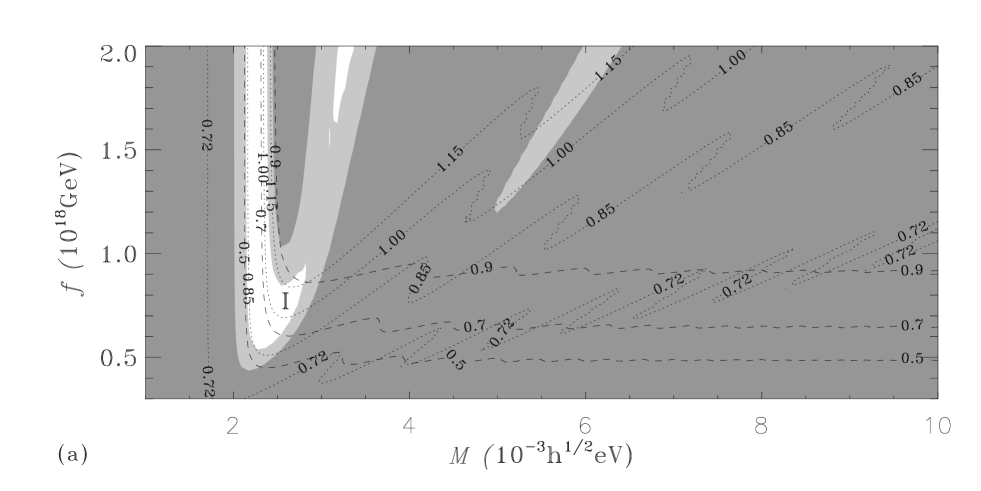
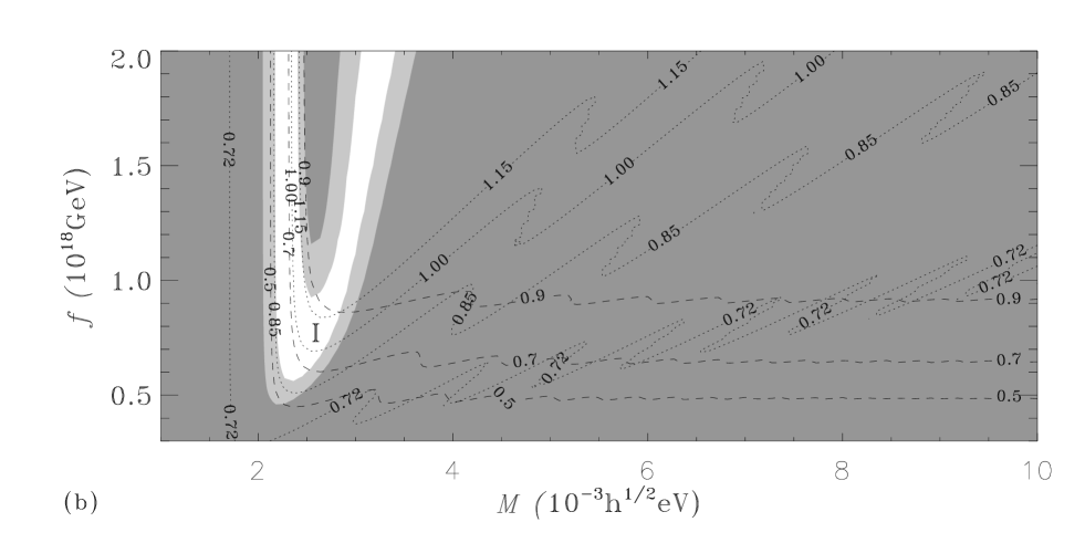
FIG. 1.: Confidence limits on $M$,$f$ parameter values, with $w_{i}=0.2$: (a) for the 60 supernovae Ia in the P98 data set; (b) for the 54 supernovae Ia in the reduced “fit C” P98 data set. Parameter values excluded at the 95.4% level are darkly shaded, while those excluded at the 68.3% level are lightly shaded. Overplotted are the contours for $\Omega_{\phi 0}$ (dashed) and $H_{0}t_{0}$ (dotted).

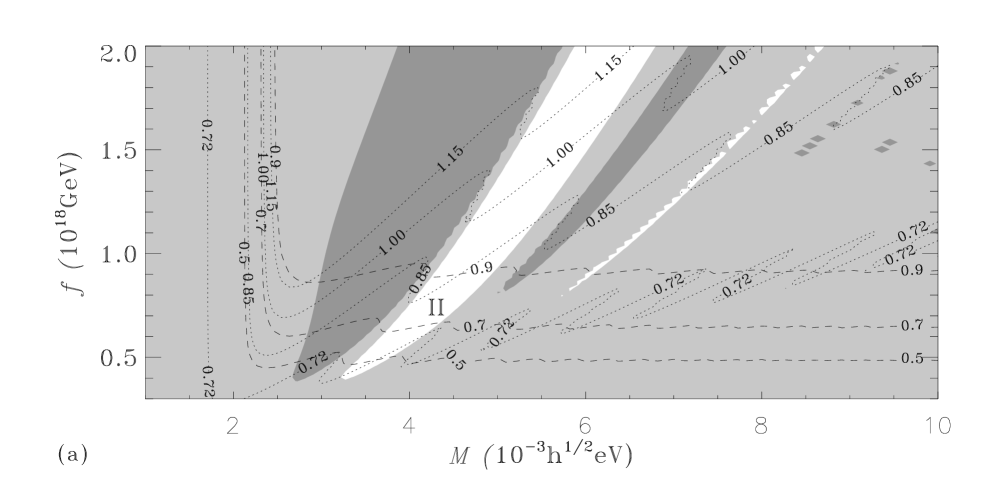
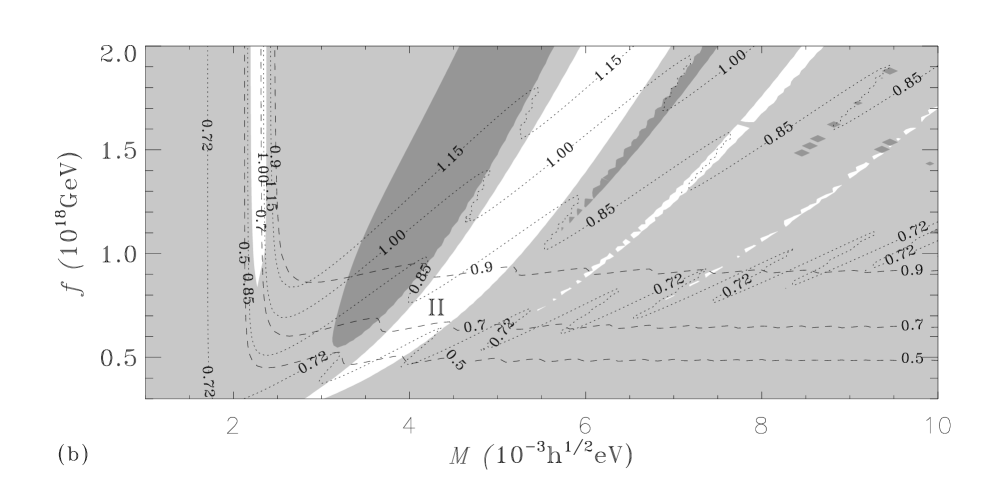
FIG. 2.: Confidence limits on $M$,$f$ parameter values, with $w_{i}=0.2$, marginalized over a flat prior for the luminosity evolution parameter $\beta$: (a) for the 60 supernovae Ia in the P98 data set; (b) for the 54 supernovae Ia in the reduced “fit C” P98 data set. Parameter values excluded at the 95.4% level are darkly shaded, while those excluded at the 68.3% level are lightly shaded. Overplotted are the contours for $\Omega_{\phi 0}$ (dashed) and $H_{0}t_{0}$ (dotted).

Here we will take a somewhat different approach to ref. [13] in our treatment of the case with source evolution. We will assume that the parameter $\beta$ has a flat prior bounded over some range $\Delta\beta=2.3$, with limits corresponding to $-0.6<\beta<1.7$, and marginalize the likelihood function over this prior. The choice of the bounds on $\beta$ in explained below in section IIB.

Despite the differences from the approach used in Ref. [13] the conclusions of the analysis are broadly similar, and are shown in Fig. 2. In particular, two regions of parameter space appear to be singled out: region I (see Fig. 1), which corresponds to cosmological models for which the scalar field is rolling down the potential (1) for the first time (with $\phi$ increasing) at the present epoch, and region II (see Fig. 2) in which the scalar field is rolling down the potential for the second time (with $\phi$ decreasing) at the present epoch. In the absence of any evolution the P98 data set favours Region I, whereas if evolution is allowed for then region II appears to be favoured slightly more than region I.

Note that over the entire parameter space considered, we find the value of $\hat{\beta}$ with the best fit of all is $\hat{\beta}\approx 0.622$ using the entire P98 data set, which occurs at parameter values $M=4.55\times 10^{-3}h^{1/2}$eV, $f=0.884\times 10^{18}$GeV, while for the “fit C” data set it is $\hat{\beta}\approx 0.720$, which occurs at $M=4.64\times 10^{-3}h^{1/2}$eV, $f=0.901\times 10^{18}$GeV. Averaged over the $(M,f)$ parameter space we find $\langle\hat{\beta}\rangle\approx 0.286$ for the full P98 data set, and $\langle\hat{\beta}\rangle\approx 0.348$ for the “fit C” data set. Thus in both cases the value of $\hat{\beta}$ is peaked in region II, but for the “fit C” data the overall values of $\hat{\beta}$ are somewhat larger.

The results of refs. [13, 15] were inconclusive. Ostensibly the source evolution models appeared to provide a slightly better fit. However, the extent to which they were better was not quantified statistically. One relatively straightforward way to compare the relative strengths of rival theoretical models in fitting a common set of data is by the calculation of Bayes factors [16, 39], even when the models involve different numbers of parameters. Given more parameters, one may always find a better fit to the data – however, the Bayes factor approach includes an effective “Ockham’s razor factor” which adds a weighting against the inclusion of extra parameters. The Bayes factor method may be readily applied to the results of [13, 15] to give an explicit statistic to compare the relative strengths of a cosmological explanation of the SNe Ia data versus an explanation in terms of source evolution.

In Bayesian inference, when comparing rival models $M_{i}$, each with parameters ${\cal Q}_{i}$, the likelihood for a model conditional on the data ($D$) in a model comparison calculation is equal to the average likelihood for its parameters,

$$p(D|M_{i})=\int d{\cal Q}_{i}\mbox{ }p({\cal Q}_{i}|M_{i}){\cal L}({\cal Q}_{i})\ ,$$ (2)

where $p({\cal Q}_{i}|M_{i})$ is the prior probability for ${\cal Q}_{i}$, and ${\cal L}({\cal Q}_{i})$ is the sampling probability for $D$ presuming $M_{i}$ to be true. The ratio of model likelihoods,

$$B_{ij}={p(D|M_{i})\over p(D|M_{j})}$$ (3)

is called the Bayes factor. When the prior odds does not strongly favour one model over another, the Bayes factor can be interpreted just as one would interpret an odds in betting. Kass and Raftery [39] provide a comprehensive review of Bayes factors, and the recommended interpretation is summarized in Table 1.

TABLE I.: Interpretation of Bayes Factors

$B_{ij}$	Strength of evidence for $H_{i}$ over $H_{j}$
1 to 3	Not worth more than a bare mention
3 to 20	Positive
20 to 150	Strong
$>150$	Very Strong

A P98 data set

In order to ascertain what degree of improvement could be expected with data from SNAP, we will begin by calculating Bayes factors for the existing P98 data set.

The prior ranges for parameters play an important role in Bayesian model comparison. We will make a choice of the prior ranges of parameters in the different models by the resulting values of $\Omega_{m0}$ and $H_{0}t_{0}$ that they give rise to. In particular, we will choose a conservative bound of $0.5\leq\Omega_{\phi 0}\leq 0.9$. For the expansion age of the universe we choose $0.72\leq H_{0}t_{0}\leq 1.15$: for $H_{0}=70\mbox{ km s}^{-1}\mbox{Mpc}^{-1}$ it corresponds to a conservative bound of $t_{0}\simeq 13\pm 3$ Gyr consistent with recent estimates [38]. The parameter space bounded by these two constraints is indicated by the contours of $\Omega_{m0}$ and $H_{0}t_{0}$ in Figs. 1 and 2. In the large $f$ region in region I where the contours appear to be parallel to the $f$–axis, a cut-off at $f\mathop{\sim}\limits 10^{19}$ GeV, the Planck scale, is chosen.

We calculate the average parameter likelihood by integrating ${\cal L}(M,f)$ over the prior ranges for the parameter and dividing the integral by the relevant area. For the full P98 data set the Bayes factor for the model without luminosity evolution versus the model with luminosity evolution, which is the ratio of the average parameter likelihoods, is $B\simeq 2.6$. For the reduced “fit C” data set we obtain a Bayes factor of 2.5, which is the same as far as its interpretation is concerned. Thus the data alone cannot discriminate between the two hypotheses.

B SNAP data sets

We will now simulate a data set which would be expected to be obtained by the SNAP satellite to investigate its potential for discriminating between the two possibilities. We will simulate two data sets from fiducial cosmologies chosen with parameters in each of regions I and II. In each case we will introduce a random error to the exact distance moduli to simulate a future supernova data set that has been converted to a table of effective magnitudes $m_{i}$ and redshifts $z_{i}$ of objects with a single fiducial absolute magnitude ${\cal M}_{0}$. We will consider both statistical and systematic uncertainties in the magnitudes. Typically the redshifts are known to sufficiently high precision that their uncertainties can be ignored. We assume the supernovae observed uniformly within four different redshift ranges with the following different sampling rates, which are the same as those chosen by Weller and Albrecht [29]: In the first range from $z=0$–$0.2$ we assume that there are $50$ observations, in the second and largest redshift range from $z=0.2$–$1.2$ there are $1800$ SNe and in the two high redshift bins, $z=1.2$–$1.4$ and $z=1.4$–$1.7$, there are $50$ SNe and $15$ SNe observations respectively. The statistical error in magnitude is assumed to be $\sigma_{\text{mag}}=0.15$, including both measurement error and any residual intrinsic dispersion after calibration.

For data set A, we assume there is no luminosity evolution. We choose the fiducial parameters $M=2.53\times 10^{-3}h^{1/2}$eV and $f=0.58\times 10^{18}$GeV; these parameters give $(\Omega_{m0},\Omega_{\phi 0})\approx(0.23,0.77)$ and $H_{0}t_{0}\approx 0.9$. For data set B, we assume there is a luminosity evolution and we add a term $\beta\ln(1+z)$ to the distance moduli. We choose the fiducial parameters $M=4\times 10^{-3}h^{1/2}$eV and $f=0.676\times 10^{18}$GeV. These parameters give $(\Omega_{m0},\Omega_{\phi 0})\approx(0.25,0.75)$ and $H_{0}t_{0}\approx 0.8$. The best–fit value of the parameter $\beta$ for this particular choice of $M$ and $f$ is $\hat{\beta}=0.659$ for the full data set, and $\hat{\beta}=0.727$ for the “fit C” reduced data set. We will take $\beta\approx 0.659$ as the fiducial parameter for data set B, as it is the somewhat more conservative value, representing less luminosity evolution.

The fiducial parameters for the two data sets have been deliberately chosen so as to give similar values of $\Omega_{m0},\Omega_{\phi 0}$ and $H_{0}t_{0}$ on one hand, so as to be consistent with values favoured by other observational tests. On the other hand, the fiducial parameters for data set A are centred in region I, which corresponds to a universe in which the scalar field is rolling down the potential for the first time at the present epoch, whereas the fiducial parameters for data set B are centred in region II, which corresponds to a universe in which the scalar field is rolling down the potential for the second time at the present epoch. As was discussed in [13] region I is favoured if the SNe Ia luminosity distances are true cosmological distances, whereas region II becomes significantly favoured if the data hides a simple luminosity evolution.

We will use Bayesian analysis to estimate uncertainties. Rigorous calculation of the likelihood for the quintessential parameters ${\cal Q}$ is very complicated, requiring the introduction and estimation of many additional parameters, including parameters from the light–curve model and parameters for characteristics of the individual supernovae. With several simplifying assumptions [16], the final result is relatively simple. One finds

$${\cal L}({\cal Q})\simeq{\rm e}^{-\chi^{2}/2}\ ,$$ (4)

where

$$\chi^{2}({\cal Q})=\sum_{i}{[\mu_{s,i}-\mu(z_{i};{\cal Q})]^{2}\over\sigma_{\mu,i}^{2}}\ .$$ (5)

In the above equation,

$$\mu(z_{i};{\cal Q})=5\log d_{L}(z_{i};{\cal Q})+25\$$ (6)

is the distance modulus predicted by each model with parameters ${\cal Q}$, while $\mu_{s,i}=m_{i}-{\cal M}_{0}$ is the simulated distance modulus, and its uncertainty is $\sigma_{\mu,i}=0.15$. Note that we fix Hubble parameter to $H_{0}=70\mbox{ km/s Mpc}^{-1}$ to simplify the computation.

The model with an unexpected luminosity evolution corresponds to replacing eq. (5) with

$$\chi^{2}({\cal Q},\beta)=\sum_{i}{[\mu_{s,i}-\beta\ln(1+z_{i})-\mu(z_{i};{\cal Q})]^{2}\over\sigma_{\mu,i}^{2}}\ .$$ (7)

We will marginalize over $\beta$ with a flat prior, to obtain the marginal likelihood

$${\cal L}({\cal Q})={1\over\Delta\beta}\int d\beta{\rm e}^{-\chi^{2}/2}\ .$$ (8)

The above integration can be performed by an analytic marginalization [13, 16]. We separate $q$ from $\chi^{2}$ where

$$q({\cal Q}) = -{\hat{\beta}^{2}({\cal Q})\over\bar{\sigma}^{2}}+\sum_{i}{h^{2}(z_{i};{\cal Q})\over\sigma_{i}^{2}}$$ (9)

$$= \sum_{i}{[h(z_{i};{\cal Q})-\hat{\beta}({\cal Q})\ln(1+z_{i})]^{2}\over\sigma_{\mu,i}^{2}}$$ (10)

is independent of $\beta$. The integral is thus an integral over a Gaussian in $\beta$ located at $\hat{\beta}$ with standard deviation $\bar{\sigma}$. $\hat{\beta}$ is the best–fit value of $\beta$ given ${\cal Q}$, and $\bar{\sigma}$ is its conditional uncertainty. They are given by

$${1\over\bar{\sigma}^{2}} = \sum_{i}{[\ln(1+z_{i})]^{2}\over\sigma_{\mu,i}^{2}}\ ,$$ (11)

$$\hat{\beta}({\cal Q}) = \bar{\sigma}^{2}\left[\sum_{i}{h(z_{i};{\cal Q})\ln(1+z_{i})\over\sigma_{\mu,i}^{2}}\right]\ ,$$ (12)

where

$$h(z_{i};{\cal Q})=\mu_{s,i}-\mu(z_{i};{\cal Q})\ .$$ (13)

As long as $\beta$ is inside the prior range and $\bar{\sigma}\ll\Delta\beta$, the value of the integral is well approximated by $\bar{\sigma}\sqrt{2\pi}$, so that

$${\cal L}({\cal Q})={\bar{\sigma}\sqrt{2\pi}\over\Delta\beta}{\rm e}^{-q/2}\ .$$ (14)

The question of what bounds to place on the prior range for the parameter $\beta$ is an interesting one, since we are dealing with a purely empirical model of source evolution with no a priori restrictions on $\beta$, other than that very large values of $\beta$ would not be physically plausible. We will therefore seek the narrowest range of values of $\beta$ consistent with our numerical results. One condition on the prior range for $\beta$ is that $\hat{\beta}$ also lies inside the prior range: setting too tight a bound on $\Delta\beta$ would count against parameter values of $M$ and $f$ which might otherwise be included. By explicit numerical integration we have found that for the initial conditions and the range of parameter values of $M$ and $f$ we have considered $\hat{\beta}$ lies in the range $-0.6<\hat{\beta}<1.7$. We will therefore take these bounds to be the prior range for $\beta$.

If we fit the data set obtained from fiducial model A assuming that there is no luminosity evolution, the parameters $M$ and $f$ are well constrained by the simulated data. The 95.4% confidence level contour bounds a very small region around the best–fit values of $M\approx 2.55\times 10^{-3}h^{1/2}$eV and $f\approx 0.592\times 10^{18}$GeV, with $\chi^{2}=1910$. These best–fit parameters are very close to the fiducial parameters that generate the data set. The average parameter likelihood is ${\cal L}_{\text{ave}}\simeq 7.1\times 10^{-4}{\cal L}_{0}$, where ${\cal L}_{0}=\exp(-1910/2)$. If luminosity evolution is considered to exist (see Fig. 3), fitting the data set from fiducial model A we find that the 95.4% confidence level contour includes a larger region in region I of the parameter space around the fiducial parameters, and a region in region II. The average parameter likelihood is ${\cal L}_{\text{ave}}\simeq 1.9\times 10^{-3}{\cal L}_{0}$. Hence, the Bayes factor for the model with luminosity evolution versus the model without luminosity evolution is $B\simeq 2.7$. We conclude that it is not possible to discriminate between the two hypotheses even though the underlying simulated data does not have any luminosity evolution.

FIG. 3.: Confidence limits on $M$,$f$ parameter values, with $w_{i}=0.2$, marginalized over a flat prior for the luminosity evolution parameter $\beta$, for the 1915 supernovae simulated assuming $M=2.53\times 10^{-3}h^{1/2}$eV, $f=0.58\times 10^{18}$GeV, and $\beta=0$. Parameter values excluded at the 95.4% level are darkly shaded, while those excluded at the 68.3% level are lightly shaded. Overplotted are the contours for $\Omega_{\phi 0}$ (dashed) and $H_{0}t_{0}$ (dotted).

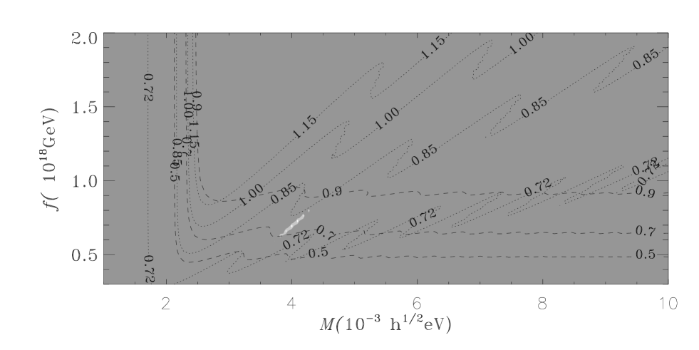
FIG. 4.: Confidence limits on $M$,$f$ parameter values, with $w_{i}=0.2$, marginalized over a flat prior for the luminosity evolution parameter $\beta$, for the 1915 supernovae simulated assuming $M=4\times 10^{-3}h^{1/2}$eV, $f=0.676\times 10^{18}$GeV, and $\beta=0.659$. Parameter values excluded at the 95.4% level are darkly shaded, while those excluded at the 68.3% level are lightly shaded. Overplotted are the contours for $\Omega_{\phi 0}$ (dashed) and $H_{0}t_{0}$ (dotted).

If we fit the data set obtained from the fiducial model B by assuming that there is no luminosity evolution, then the 95.4% level bounds a very small region around the best–fit values of $M\approx 2.27\times 10^{-3}h^{1/2}$eV and $f\approx 0.764\times 10^{18}$GeV. The average parameter likelihood is ${\cal L}_{\text{ave}}\simeq 9.4\times 10^{-18}{\cal L}_{0}$, where ${\cal L}_{0}=\exp(-1924/2)$. If luminosity evolution is considered to exist (see Fig. 4), on the other hand, then the 95.4% level bounds a small region around the best–fit values of $M\approx 4.00\times 10^{-3}h^{1/2}$eV and $f\approx 0.695\times 10^{18}$GeV, with $\hat{\beta}\approx 0.626$ and normalized $\chi^{2}=1924$. The average parameter likelihood is ${\cal L}_{\text{ave}}\simeq 8.3\times 10^{-4}{\cal L}_{0}$. This time, the Bayes factor for the model with luminosity evolution relative to the model without luminosity evolution is much greater than one, $B\simeq 9.1\times 10^{13}$. Thus if the true data were derived from fiducial model B, it would show up clearly as giving a $d_{L}(z)$ which can be discriminated from the model without luminosity evolution.

This result in no way contradicts the inconclusive result obtained from data set A. If the underlying data were to truly follow a simple luminosity evolution, then the analysis above shows that this would stand out as a very strong positive signal in the Bayes factor test. If the underlying data has no luminosity evolution on the other hand, then it may be possible to obtain a good fit with an extra luminosity evolution parameter, simply because one has an extra parameter to fit. Thus a simple luminosity evolution is easy to rule in, but difficult to rule out. Combined together the two results demonstrate the efficacy of the Bayes factor approach. With data set B we would obtain a decisive result, but by Ockham’s razor we should reject the more complicated evolutionary hypothesis if we were to obtain an inconclusive result such as that pertaining to data set A. In fact, we have found that by narrowing the range of the prior $\Delta\beta$ that the Bayes factor for data set A can even be made slightly greater than the cut-off value of 3 listed in Table 1. Clearly any weakly positive results should therefore also be treated with some caution.

III PNGB versus other potentials

The constraints on cosmological parameters which arise from type Ia supernovae have been broadly studied for a wide range of quintessence models [11, 12, 13, 15]. However, all these models seem to have ranges of parameters that fit the existing data equally well, with no particular model standing out as being observationally preferred. The lack of data and the large statistical error bars are among the contributing reasons. In this section, we will investigate the potential of the SNAP supernovae data set to discriminate between competing quintessence models, as contrasted with the P98 data set, assuming no source evolution.

We consider some simple scalar field potential functions which have been widely studied in the literature. They are the simple exponential potential [7, 12, 22]

$$V=V_{A}{\rm e}^{-\lambda\kappa\phi}\ ,$$ (15)

the inverse power–law potential [8, 23]

$$V=V_{A}\phi^{-\alpha}\ ,$$ (16)

and the double–exponential potential [12, 24]

$$V=V_{A}\exp(-A\,{\rm e}^{\sqrt{2}\kappa\phi})\ ,$$ (17)

where $\kappa$ is related to Newton’s constant by $\kappa^{2}=8\pi G$. We evaluate the luminosity distance – redshift relation by numerically evolving the Einstein-scalar field evolution equations forward from the time of onset of matter domination, as what we did for the PNGB models. For the simple exponential and the double–exponential potentials, without lost of generality we choose the initial condition $\phi_{i}=0$. For the power–law potential, we begin the integration by assuming that the scalar field has already reached the tracker solution. These leave us with two parameters in each case. In Figs. 5, 6, and 7, we display the confidence limits for the 54 supernovae Ia in the P98 “fit C” reduced data set, on the parameter spaces for these quintessence models. (The equivalent figures for the full data set have been omitted, as the 1$\sigma$ and 2$\sigma$ confidence regions are very similar to those shown in Figs. 5–7, but just slightly narrower.)

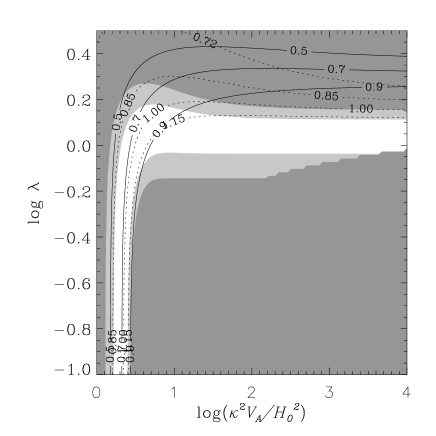
FIG. 5.: Confidence limits on the parameter space for the simple exponential potential model $V=V_{A}{\rm e}^{-\lambda\kappa\phi}$, for the 54 supernovae Ia in the P98 “fit C” reduced data set. Parameter values excluded at the 95.4% level are darkly shaded, while those excluded at the 68.3% level are lightly shaded. Overplotted are the contours for $\Omega_{\phi 0}$ (solid) and $H_{0}t_{0}$ (dotted).

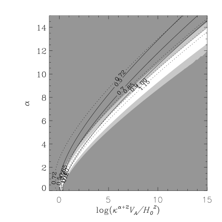
FIG. 6.: Confidence limits on the parameter space for the inverse power–law potential model $V=V_{A}\phi^{-\alpha}$, for the 54 supernovae Ia in the P98 “fit C” reduced data set. Parameter values excluded at the 95.4% level are darkly shaded, while those excluded at the 68.3% level are lightly shaded. Overplotted are the contours for $\Omega_{\phi 0}$ (solid) and $H_{0}t_{0}$ (dotted).

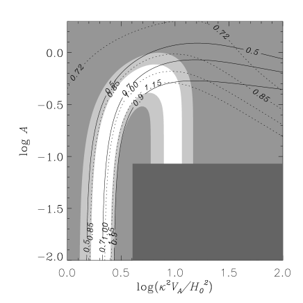
FIG. 7.: Confidence limits on the parameter space for the double–exponential potential model $V=V_{A}\exp(-A{\rm e}^{\sqrt{2}\kappa\phi})$, for the 54 supernovae Ia in the P98 “fit C” reduced data set. Parameter values excluded at the 95.4% level are darkly shaded, while those excluded at the 68.3% level are lightly shaded. Overplotted are the contours for $\Omega_{\phi 0}$ (solid) and $H_{0}t_{0}$ (dotted). The lower right-hand region is excluded from the plot due to computational difficulties.

In this section we will only compare models (15)–(17) on the basis of assuming that the true data follows the PNGB model, with the fiducial parameters of data set A. Naturally, we could assume any of the other potentials (15)–(17) as our fiducial model, and then compare the other models on the basis of a new fiducial data set. This would allow us, for example, to compare the inverse power–law potential (16) with the simple– and double–exponential potentials (15), (17), a test which we have not performed here. However, we will restrict our attention to the fiducial data set A relevant to the PNGB potential (1), since the amount of computer time involved in computing the fiducial data sets is large, and an analysis based on a fiducial PNGB model will prove to be sufficient to illustrate the dramatically increased discriminatory power of a SNAP dataset as opposed to presently available SNe Ia data. Naturally, one could extend the discussion to other fiducial data sets, but we will leave that to future work.

A P98 data set

Firstly we will calculate the Bayes factor of the P98 data set to compare the PNGB model with all the other quintessence models. In order to calculate Bayes factors which compare different theoretical models we must naturally make choices of the range of prior parameters integrated over, and we are dealing with different parameters in the different models. Different choices of priors for these parameters would lead to some variation in the resulting Bayes factors. We will make a choice of the range of prior parameters by using the resulting values of $\Omega_{\phi 0}$ and $H_{0}t_{0}$ that they give rise to. However, the parameter spaces are not completely bounded by the $\Omega_{\phi 0}$ and $H_{0}t_{0}$ constraints. Without a physical cut-off for the parameters, such as a cut-off for $f$ at Planck scale for the PNGB model, we will investigate in each case the dependence of the Bayes factor comparison on the prior ranges of the parameters. We will show that in some cases, the choice of the prior parameter ranges do not affect the conclusion from the Bayes factor analysis.

For the simple exponential potential model, as shown in Fig. 5, the $\Omega_{\phi 0}$ and $H_{0}t_{0}$ contours diverge at large $V_{A}$, putting a bound on the parameter space. In the small $\lambda$ region, where the potential is effectively a cosmological constant model whose value depends on $V_{A}$ only, the $\Omega_{\phi 0}$ and $H_{0}t_{0}$ contours remain near parallel. For the full P98 data set the average parameter likelihood over the region bounded by the $\Omega_{\phi 0}$ and $H_{0}t_{0}$ constraints, with a cut-off at $\lambda=0.1$, is ${\cal L}_{\text{ave}}\simeq 0.67{\cal L}_{R}$, where ${\cal L}_{R}$ is the average parameter likelihood for the PNGB model. In the small $\lambda$ region the likelihood only changes slightly with decreasing $\lambda$ and tends to a constant, corresponding to an average parameter likelihood which we estimate to be ${\cal L}_{\text{ave}}\simeq 1.5{\cal L}_{R}$. Since the small $\lambda$ region extends to an infinite range in terms of the parameterization shown in Fig. 5, if we enlarge the prior range of $\lambda$ to include smaller values, then it has the effect of bringing the average parameter likelihood closer to the average parameter likelihood in the small $\lambda$ region, which is effectively an upper bound. Thus the Bayes factor for the simple exponential potential model versus the PNGB model lies in the range $0.67<B<1.5$ for the full P98 data set. Similarly $0.65<B<1.5$ for the reduced “fit C” data set. In each case the larger value is the one appropriate to including the entire small parameter range for $\lambda$. Such a Bayes factor is too small to confidently discriminate between the two models.

For the double–exponential potential model, the average parameter likelihood over the region bounded by the $\Omega_{\phi 0}$ and $H_{0}t_{0}$ constraints, with a cut-off at $A=0.01$, is ${\cal L}_{\text{ave}}\simeq 0.92{\cal L}_{R}$ for the full P98 data set. The average parameter likelihood in the small $A$ region, where the potential is effectively a cosmological constant model whose value depends on $V_{A}$ only, is ${\cal L}_{\text{ave}}\simeq 1.5{\cal L}_{R}$. By a similar argument to above, the Bayes factor for the double–exponential potential model versus the PNGB model varies slightly over a range $0.92<B<1.5$ for the full P98 data set. Similarly, $0.38<B<1.5$ for the reduced “fit C” data set. Again, the Bayes factor is too small to confidently discriminate between the two models.

For the inverse power–law potential model, as shown in Fig. 6, the $\Omega_{\phi 0}$ and $H_{0}t_{0}$ contours remain nearly parallel towards the upper right-hand region where both $V_{A}$ and $\alpha$ are large. The average parameter likelihood over the region bounded by the $\Omega_{\phi 0}$ and $H_{0}t_{0}$ constraints with arbitrary cut-offs at $\kappa^{\alpha+2}V_{A}/H_{0}^{2}=10^{15}$ and $\alpha=15$ is ${\cal L}_{\text{ave}}\simeq 0.14{\cal L}_{R}$ for the full P98 data set, and ${\cal L}_{\text{ave}}\simeq 0.11{\cal L}_{RC}$ for the reduced “fit C”data set, where ${\cal L}_{RC}$ is the average parameter likelihood for the PNGB model based on the “fit C” data set. This gives a Bayes factor for the PNGB model versus the inverse power–law potential model of $B=7.2$ for the full P98 data set, or $B=9.2$ for the “fit C” data set. Both values are large enough to provide slightly positive evidence that the P98 data set favours the PNGB model over the inverse power–law potential model. Since the Bayes factor is only weakly positive, however, we cannot not place strong confidence in this conclusion. Note that the $\Omega_{\phi 0}$ and $H_{0}t_{0}$ contours both extend towards the smaller likelihoods region. Therefore, increasing the prior ranges for $V_{A}$ and $\alpha$ will decrease the average parameter likelihood, and increase the slightly positive preference for the PNGB potential as compared to the inverse power–law potential in the Bayes factor test.

B SNAP data set

We have shown that the P98 data set does not particularly favour any of the PNGB, simple exponential potential, and double–exponential potential models relative to the others. The P98 data set does disfavour the inverse power–law potential model as compared with the PNGB model. This might be considered to result from the fact that the $2\sigma$–confidence region only overlaps with a small region (the low $\alpha$ region) of the whole parameter space allowed by the priors set on $\Omega_{\phi 0}$ and $H_{0}t_{0}$.

In this section we want to compare the typical results we should expect when a future SNAP data set is used. We will use data set A, simulated from a fiducial PNGB model assuming no luminosity evolution. We will study the potential of this data set to distinguish the PNGB model from other quintessence models.

For the simple exponential potential model, the average parameter likelihood over the region bounded by the $\Omega_{\phi 0}$ and $H_{0}t_{0}$ constraints, with a cut-off at $\lambda=0.1$, is ${\cal L}_{\text{ave}}\simeq 2.1\times 10^{-5}{\cal L}_{0}$, where ${\cal L}_{0}=\exp(-1910/2)$. In the small $\lambda$ region, we estimate the average parameter likelihood to be ${\cal L}_{\text{ave}}\simeq 6.6\times 10^{-31}{\cal L}_{0}$. Comparing with the average parameter likelihood for the PNGB model, ${\cal L}_{\text{ave}}\simeq 7.1\times 10^{-4}{\cal L}_{0}$, the Bayes factor for the PNGB model versus the simple exponential potential model takes values in the range $34$ – $10^{27}$, depending on the prior range for $\lambda$. This would provide a very strong conclusion that data set A favours the PNGB model over the simple exponential potential model.

For the double–exponential potential model, the average parameter likelihood over the region bounded by the $\Omega_{\phi 0}$ and $H_{0}t_{0}$ constraints, with a cut-off at $A=0.01$, is ${\cal L}_{\text{ave}}\simeq 1.6\times 10^{-3}{\cal L}_{0}$. The average parameter likelihood in the small $A$ region, is ${\cal L}_{\text{ave}}\simeq 2.1\times 10^{-29}{\cal L}_{0}$. The Bayes factor for the PNGB model versus the double–exponential potential model lies in the range $0.44$ – $10^{25}$, depending on the the prior range for $A$. The lower bound of the Bayes factor, $B=0.44$, is too small to confidently discriminate between the two models. However, provided small values of the parameter $A$ are included in the prior range, the Bayes factor would provide a strong conclusion that data set A favours the PNGB model over the double–exponential potential model.

For the inverse power–law potential model, the average parameter likelihood over the region bounded by the $\Omega_{\phi 0}$ and $H_{0}t_{0}$ constraints with arbitrary cut-offs at $\kappa^{\alpha+2}V_{A}/H_{0}^{2}=10^{15}$ and $\alpha=15$ is ${\cal L}_{\text{ave}}\simeq 1.9\times 10^{-10}{\cal L}_{0}$. This gives a Bayes factor for the PNGB model versus the inverse power–law potential model of $B\simeq 10^{6}$. This provides very strong evidence that data set A would favour the PNGB model over the inverse power–law potential model.

IV Discussion

Let us now consider our results in relation to previous work concerning the feasibility of determining the properties of the dark energy from future supernovae surveys [25, 27, 28, 29, 30, 31]. One approach in past studies of scalar field quintessence has been to assume a potential $V(\phi)$ over which the scalar field, $\phi$, would have slowly varied during cosmological time scales, and then test the efficacy of reconstructing the potential [25, 27]. Another approach has been to assume that the quintessence field can be described by a perfect fluid with slowly varying equation of state $P=w(z)\rho$, expand $w(z)$ in a power series, and then test the efficacy of determining the coefficients in the power series [28, 29, 30, 31].

The conclusions of investigations to date are mixed [28, 29, 30, 31]. Weller and Albrecht [29] find that many models can be distinguished with a fit to a linear equation of state for the dark energy, $P=w(z)\rho$ with $w(z)=w_{0}+w_{1}z$, but only if the current mass density, $\Omega_{m}$, is known to a high precision. Barger and Marfatia [30] find that, even by putting $\Omega_{m}=0.3$ exactly, there is still a possibility of obtaining data sets which might not discriminate between quintessence and “$k$-essence”, namely an alternative form of dark energy with a scalar field characterized by non-linear kinetic terms [40]. Wang and Garnavich [31] consider two classes of functions $w(z)$, corresponding respectively to a linear variation and to $k$-essence. Using somewhat different techniques to other authors they are more optimistic about prospects for determining $w(z)$ from future SNe Ia data.

In the present paper we have taken a different approach from those above, by considering a class of models – the PNGB models – which are very well motivated from the point of view of particle physics, but for which the above methods will not always be satisfactory in the case of all plausible parameter ranges, given the potentially oscillatory nature of $w(z)$ and the corresponding fact that the scalar field may have varied over a wide range of values of $V(\phi)$ over observable time scales. We fitted the simulated SNAP data sets to the exact $d_{L}(z)$ of different models obtained by numerical integration, and compared them to other models.

One real drawback of all approaches is that as yet there is no preferred physical model for the dark energy. On one hand this means that any approximations made in potential reconstruction methods may be too restrictive, since many different potential energy functions $V(\phi)$ are conceivable, and many of these may give results degenerate with each other. On the other hand, using a given Lagrangian for the quintessence field, as we have done, limits us to a model by model test.

Nevertheless, we find that data sets such as those that would be produced by SNAP promise to be very successful on some tests, even if they will probably be less successful on others. In particular, while existing data is not yet sufficiently large to discriminate between various quintessence models or models with evolution [11, 12, 13], we have shown that the much larger size and smaller error bars of the simulated SNAP type IA supernovae data sets provide much tighter constraints on the parameters for quintessence models such as those corresponding to pseudo Nambu–Goldstone bosons.

By evaluating Bayes factors in the context of the PNGB model, we have shown that future satellite SNe Ia data sets should have greater success in detecting whether the observed luminosity distance – redshift relation is purely cosmological in origin, or is significantly contaminated by evolutionary effects of the sources. The results of section IIB showed that although it may be difficult to completely rule out luminosity evolution, if the true data were from a population with luminosity evolution then this would provide a strong distinctive signal. We have only studied one simple illustrative supernova luminosity evolution function, but we expect that similar conclusions would apply to other simple luminosity evolution models.

We have further shown that with the future data it should be possible to discriminate PNGB model from some other particular types of quintessence; in particular, it gives a very different signature to that of simple inverse power–law potentials or simple exponential potentials. The case of a double–exponential potential gives a lower Bayes factor, and may therefore be more difficult to distinguish from the PNGB model. However, even in this case some distinction between the two models is possible if one allows a suitably large prior range of the parameter $A$, to include small values.

A number of obvious extensions of our analysis are possible. In the case of testing source evolution versus the case with no evolution, for example, it would be interesting to determine by how much we can reduce the parameter $\beta$ for the simulated SNAP data set B while still obtaining a very strong result for the discriminatory power of the relevant Bayes factor. Given the magnitude of the value obtained in section IIB, we suspect that the fiducial value of $\beta$ could be significantly reduced. Likewise many other tests could be performed with fiducial data sets based on other quintessence potentials.

In conclusion, we find that future supernovae measurements such as those that would be afforded by the SNAP satellite, will have the power to significantly increase our knowledge of the properties of the dark energy in the universe. To be completely confident, however, we will require a deeper theoretical understanding of the nature of the dark energy and hopefully new input from fundamental physics.

REFERENCES

- [1] Electronic address: cng@physics.adelaide.edu.au
- [2] Electronic address: dlw@phys.canterbury.ac.nz
- [3] Present address
- [4] S. Perlmutter et al., Astrophys. J. 483, 565 (1997).
- [5] A.G. Riess et al., Astron. J. 116, 1009 (1998).
- [6] S. Perlmutter et al., Astrophys. J. 517, 565 (1999).
- [7] C. Wetterich, Nucl. Phys. B302, 668 (1988).
- [8] P.J.E. Peebles and B. Ratra, Astrophys. J. 325, L17 (1988); Phys. Rev. D37, 3406 (1988).
- [9] R.R. Caldwell, R. Dave, and P.J. Steinhardt, Phys. Rev. Lett. 80, 1582 (1998).
- [10] See P. Binetruy, Int. J. Theor. Phys. 39, 1859 (2000), and references therein.
- [11] I. Waga and A.P. Miceli, Phys. Rev. D59, 103507 (1999); S. Perlmutter, M.S. Turner, and M. White, Phys. Rev. Lett. 83, 670 (1999); L. Wang, R.R. Caldwell, J.P. Ostriker, and P.J. Steinhardt, Astrophys. J. 530, 17 (2000); S. Podariu and B. Ratra, Astrophys. J. 532, 109 (2000); J.A. Frieman and I. Waga, Phys. Rev. D57, 4642 (1998). I. Waga and J.A. Frieman, Phys. Rev. D62, 043521 (2000); R.G. Vishwakarma, Class. Quantum Grav. 18, 1159 (2001).
- [12] S.C.C. Ng, Phys. Lett. B485, 1 (2000).
- [13] S.C.C. Ng and D.L. Wiltshire, Phys. Rev. D63, 023503 (2001).
- [14] A.G. Riess, A.V. Filippenko, W. Li and B.P. Schmidt, Astron. J. 118, 2668 (1999).
- [15] D.L. Wiltshire, in Cosmology and Particle Physics, Proceedings of the CAPP’2000 Conference, Verbier, Switzerland, eds. J. García-Bellido, R. Durrer and M. Shaposhnikov, (American Institute of Physics, 2001) p. 555 [=astro-ph/0010443].
- [16] P.S. Drell, T.J. Loredo, and I. Wasserman, Astrophys. J. 530, 593 (2000).
- [17] A.G. Riess et al., astro-ph/0104455.
- [18] http://www.snap.lbl.gov
- [19] For an earlier proposal on similar lines see: Y. Wang, Astrophys. J. 531, 676 (2000).
- [20] C.T. Hill and G.G. Ross, Nucl. Phys. B311, 253 (1988); Phys. Lett. B203, 125 (1988).
- [21] J.A. Frieman, C.T. Hill, A. Stebbins and I. Waga, Phys. Rev. Lett. 75, 2077 (1995).
- [22] See, for example, E.J. Copeland, A.R. Liddle, and D. Wands, Phys. Rev. D57, 4686 (1998); P.G. Ferreira and M. Joyce, Phys. Rev. Lett. 79, 4740 (1997); Phys. Rev. D58, 023503 (1998), and references therein.
- [23] I. Zlatev, L. Wang and P.J. Steinhardt, Phys. Rev. Lett. 82, 896 (1999); P.J. Steinhardt, L. Wang and I. Zlatev, Phys. Rev. D59, 123504 (1999).
- [24] P. Binetruy, Phys. Rev. D60, 063502, (1999); A. de la Macorra, hep-ph/9910330 (1999).
- [25] A.A. Starobinsky, Pis’ma Zh. Éksp. Teor. Fiz. 68, 721 (1998) [JETP Lett. 68, 757 (1998)]; T.D. Saini, S. Raychaudhury, V. Sahni and A.A. Starobinsky, Phys. Rev. Lett. 85, 1162 (2000).
- [26] V. Sahni and L. Wang, Phys. Rev. D62, 103517 (2000).
- [27] D. Huterer and M.S. Turner, Phys. Rev. D60, 081301 (1999); astro-ph/0012510; T. Chiba and T. Nakamura, Phys. Rev. D62, 121301 (2000).
- [28] I. Maor, R. Brustein, and P.J. Steinhardt, Phys. Rev. Lett. 86, 6 (2001); M. Goliath, R. Amanullah, P. Astier, A. Goobar, and R. Pain, astro-ph/0104009; J. Weller and A. Albrecht, astro-ph/0106079.
- [29] J. Weller and A. Albrecht, Phys. Rev. Lett. 86, 1939 (2001).
- [30] V. Barger and D. Marfatia, Phys. Lett. B498, 67 (2001).
- [31] Y. Wang and P.M. Garnavich, Astrophys. J. 552, 445 (2001).
- [32] A.E. Lange et al., Phys. Rev. D63, 042001 (2001); C.B. Netterfield et al., astro-ph/0104460.
- [33] A. Balbi et al., Astrophys. J. 545, L1 (2000); R. Stompor et al., Astrophys. J. 561, L7 (2001).
- [34] C. Pryke et al., astro-ph/0104490.
- [35] Phillips, M.M., Astrophys. J. 413, L105 (1993).
- [36] Hamuy, M., et al., Astron. J. 112, 2391 (1996).
- [37] Riess, A.G., Press, W.H., and Kirshner, R.P. Astrophys. J. 473, 88 (1996).
- [38] O. Lahav, astro-ph/0105352.
- [39] R.E. Kass and A.E. Raftery, J. Am. Statist. Assoc. 90, 773 (1995).
- [40] T. Chiba, T. Okabe and M. Yamaguchi, Phys. Rev. D62, 023511 (2000); C. Armendariz-Picon, V. Mukhanov, and P.J. Steinhardt, Phys. Rev. Lett. 85, 4438 (2000); Phys. Rev. D63, 103510 (2001).