Constrained Simulations of the Real Universe: the Local Supercluster

Abstract

We present cosmological simulations which closely mimic the real Universe within $\sim 100$ Mpc of the Local Group. The simulations, called Constrained Simulations, reproduce the large-scale density field with major nearby structures, including the Local Group, the Coma and Virgo clusters, the Great Attractor, the Perseus-Pices, and the Local Supercluster, in approximately correct locations. The MARK III survey of peculiar velocities of the observed structures inside $80\mbox{$h^{-1}$Mpc}$ sphere is used to constrain the initial conditions. Fourier modes on scales larger then a (Gaussian) resolution of $\approx R_{g}=5\mbox{$h^{-1}$Mpc}$ are dominated by the constraints, while small scale waves are essentially random. The main aim of this paper is the structure of the Local Supercluster region (LSC; $\sim 30\mbox{$h^{-1}$Mpc}$ around the Virgo cluster) and the Local Group environment. We find that at the current epoch most of the mass ($\approx 7.5\times 10^{14}\mbox{$h^{-1}$M${}_{\odot}$}$) of the LSC is located in a filament roughly centered on the Virgo cluster and extending over $\sim 40\mbox{$h^{-1}$Mpc}$. The simulated Local Group (LG) is located in an adjacent smaller filament, which is not a part of the main body of the LSC, and has a peculiar velocity of $\approx 250~{}\rm km\ s^{-1}$ toward the Virgo cluster. The peculiar velocity field in the LSC region is complicated and is drastically different from the field assumed in the Virgocentric infall models. We find that the peculiar velocity flow in the vicinity of the LG in the simulation is relatively “cold”: the peculiar line-of-sight velocity dispersion within $7\mbox{$h^{-1}$Mpc}$ of the LG is $\lesssim 60~{}\rm km\ s^{-1}$, comparable to the observed velocity dispersion of nearby galaxies.

1 Introduction

Over the last two decades cosmological simulations have proved to be an invaluable tool in testing theoretical models in the highly nonlinear regime. However, comparisons of simulations with observational data are typically done only in a statistical sense. The standard approach is to assume a cosmological model and to use the appropriate power spectrum of the primordial perturbations to construct a random realization of the density field within a given simulation volume. The evolution of the initial density field is then followed using a numerical code and results are compared with observations. A wide variety of statistical measures has been used for comparisons, including the two-point correlation function, the power spectrum, the mass function, different shape statistics, etc.

The statistical approach works well if there is a statistically representative sample of objects with well understood selection effects for both the observed Universe and the simulations. The number of sample objects should be sufficient to overcome the cosmic variance. The approach fails, however, in cases dealing with rare objects such as the Great Attractor or specific configurations as, for example, in the problem of the local peculiar velocity field (Peebles, 1992). The traditional solution has been to choose “observers” or regions in the simulations that resemble the desired configuration as closely as possible. The results of numerical simulations aimed at identifying structures similar to those observed locally in random realizations of the initial density field were generally inconclusive because one is never sure that the selection of objects in simulations is right.

The catalog of galaxy groups constructed using the CfA redshift survey (Davis et al., 1982) is a good illustration of the difficulties one encounters in comparing model predictions to observations (Huchra & Geller, 1982; Nolthenius et al., 1997). While the data-set was sufficiently large for statistical comparisons with models, a large fraction of groups in the sample is in one large object: in the Local Supercluster (LSC). For detailed comparison with observational data it was important to identify groups in a similar environment in cosmological simulations. For example, it was crucial to mimic the environment of the Local Group (LG) in the LSC (e.g., Nolthenius et al., 1997). This was done by simply choosing an “observer” $20\mbox{$h^{-1}$Mpc}$ away from a cluster with mass comparable to that of the Virgo Cluster. Unfortunately, it is not clear what “similar environment” actually means and that simply placing the “observer” at some distance from “Virgo” cluster resolves the issue.

Another problem that is not easy to address using statistical comparisons is the peculiar velocity field around the LG. The observed low velocities of nearby galaxies have long being perceived as one of the important challenges for structure formation models (Peebles, 1992). Because we deal with rather specific environment, in simulations we must find objects, which are analogous to the real Local Group. The interpretation of the galaxy velocity field is further complicated by the possibility of velocity bias (Gelb & Bertschinger, 1994; Colín et al., 2000). Nevertheless, it was suggested that, even after taking the uncertainties into account, observed peculiar velocities of galaxies around the LG are unusually low if compared to the typical velocities of galaxies in cosmological simulations (Schlegel et al., 1994; Governato et al., 1997).

There are two possible ways of addressing problems, which require comparison with specific astronomical objects or with specific environments. (i) We may simply ignore them and wait for larger observational data-sets, such as the Sloan Digital Sky Survey, and pursue the statistical comparison of the observed data with the theoretical predictions. Clearly, the increasing amount and quality of data will continue to fuel the statistical way of testing the cosmological models. At the same time, observational data always will be more extensive and more complete for nearby, somewhat unique objects. Thus, by doing only statistical tests we are bound to lose information on the best observed astronomical objects in our sample.

(ii) An alternative approach, adopted in the present study, is to find a way of making simulations, which reproduce the large scale structures of the real Universe, while keeping the initial conditions consistent with the power spectrum of a given cosmological model. In particular, we want to simulate the small scale nearby structures within the correct large environment of the real Universe as revealed by various large scale surveys. This is done by setting initial conditions of the simulations by constrained realizations of Gaussian fields (Hoffman & Ribak, 1991), thereby constructing the density and velocity fields which agree both with the observed large scale structures and with the assumed theoretical model. This approach is called here as constrained simulation (CS).

Low resolution CSs were made before by Kolatt et al. (1996) and Bistolas & Hoffman (1998), using the IRAS 1.2Jy redshift survey to set the constraints, with the main aim of producing a semi-realistic non-linear realization of the large scale structure. Recently, such CSs were made using the MARK III survey of radial velocities (Willick et al., 1997), and were used (van de Weygaert & Hoffman, 1999, 2000) to study the origin of the local cold velocity field. The study presented here extends this work by using numerical simulations of much higher spatial and mass dynamic range. The dynamic range achieved by the Adaptive Mesh Refinement simulations used in this study far exceeds the range of all previous CSs. The combination of CSs and adaptive mesh refinement is the optimal strategy for simulating formation of the local structures at high spatial and mass resolution in a computational box sufficiently large to properly model the large-scale tidal field.

The present work is the first in a series of papers studying the dynamics of the nearby universe by means of CSs. The main purpose of this paper is to present the general approach and details of the method. The specific CS analyzed here is a relatively low resolution one, while forthcoming CSs will use higher resolution initial conditions and will reach higher mass and spatial dynamic range. As an illustration, this paper addresses the question of morphology of the density field and dynamics in the LSC region. In the following sections we present analysis of the structure of the Local Supercluster, as well as the smoothness of the Hubble expansion and peculiar velocity field in the simulated LSC region. We will also discuss the accuracy of the Virgocentric model in describing the velocity field in our simulation. The upcoming studies will focus on a variety of problems, including gas-dynamic simulations of the Virgo cluster and the LSC region (Kravtsov et al., 2001), high-resolution simulation of the LG, halo/galaxy formation in the Local Void region, and biased galaxy formation in the local universe.

The paper is organized as follows. A brief review of studies of the LSC region is given in § 2. The formalism of constrained realizations, the MARK III survey, and the construction of the initial conditions are presented in § 3.1, § 3.2, and § 3.3, respectively. The details of the numerical simulation are described in § 3.4 and § 4. The analysis of the CS is presented in §5 and we conclude the paper with a discussion of the results in § 6.

2 The Local Supercluster

Ever since the first large samples of nebulae compiled by William and John Herschel, it was known that there is a marked excess of bright objects in the northern hemisphere around the Virgo cluster, with most nebulae concentrated in a wide band spanning some $100^{\circ}$ (e.g., Reynolds, 1923; Lundmark, 1927; Shapley, 1934). In 1950s de Vaucouleurs (1953, 1958) was the first to argue that this excess corresponds to a real 3-dimensional structure in galaxy distribution. At first de Vaucouleurs (1953) called the structure the “Supergalaxy” (and introduced the supergalactic coordinates in analogy with galactic coordinate system) conjecturing that the apparent flattened galaxy distribution represented a large-scale galaxy-like system. later he subsequently changed the name to the “Local Supercluster” (LSC; de Vaucouleurs, 1958), which has been used in the literature ever since.

The debate on whether the LSC is a physical system or a chance alignment of galaxies has continued over several decades (e.g., Bahcall & Joss, 1976; de Vaucouleurs, 1976, 1978) and was settled with the advent of large redshift surveys of nearby galaxies (Sandage & Tammann, 1981; Fisher & Tully, 1981; Davis et al., 1982). Yahil et al. (1980) and Tully (1982), for example, analyzed the morphology of the 3-dimensional distribution of galaxies in the Sandage & Tammann (1981) and Fisher & Tully (1981) surveys, respectively, and showed convincingly that the concentration of galaxies along the supergalactic plane on the sky does indeed correspond to a flattened large-scale structure in the distribution of nearby galaxies. Einasto et al. (1984) applied a battery of tools to quantify the statistical properties of the galaxy distribution in the LSC region and compared the results with quantitative and qualitative predictions of several cosmological models. In particular, they showed that the LSC is similar in structure and morphology to other known superclusters such as the Perseus-Pisces supercluster and is a part of the large-scale network of clusters, sheets, and filaments.

More recent studies (Tully & Fisher, 1987; Karachentsev & Makarov, 1996; Lahav et al., 2000) showed that the main body of the LSC is a filamentary structure that extends over some $40\mbox{$h^{-1}$Mpc}$ and is roughly centered on the Virgo cluster. The whole region is dominated by several clusters (Virgo, Ursa Major, and Fornax are the most prominent), groups, and filaments, the latter bordering nearby voids (such as the Local Void). The LG is located in the outskirts of this region in a small filament extending from the Fornax cluster to the Virgo cluster (Karachentsev & Makarov, 1996). The LSC contains a fair number of galaxy groups (Huchra & Geller, 1982) and its skeletal structure is well traced by radio galaxies and AGNs (Shaver & Pierre, 1989; Shaver, 1991).

The quest for the Hubble constant and the advent of peculiar velocity surveys of galaxies fueled studies of galaxy dynamics in the LSC region (see, e.g., Davis & Peebles, 1983; Huchra, 1988, and references therein). In particular, it was recognized that the infall of the LG toward the LSC could be used to measure the mass-to-light ratio (and hence the matter density in the Universe, $\Omega_{0}$) on large scales (Silk, 1974; Peebles, 1976). The Virgocentric infall model (Gunn, 1978) was used to estimate $\Omega_{0}\sim 0.2-0.3$ from the observed local peculiar flow of galaxies (Huchra, 1988). This model requires rather large non-linear corrections (Yahil, 1985; Villumsen & Davis, 1986) and was shown to be quite inaccurate when tested using outputs of numerical cosmological simulations (Villumsen & Davis, 1986; Lee et al., 1986; Cen, 1994; Governato et al., 1997), rendering the conclusions about $\Omega_{0}$ inconclusive.

The quiescence of the local peculiar velocity field (de Vaucouleurs, 1958; Sandage & Tammann, 1975; Rivolo & Yahil, 1981; Sandage, 1986; Giraud, 1986; Schlegel et al., 1994; Karachentsev & Makarov, 1996; Sandage, 1999; Ekholm et al., 2001) is a long standing puzzle which presents a challenge for models of structure formation (e.g., Peebles, 1992). That this puzzle is by no means solved is clear from the recent study by Sandage (1999) who comments that “the explanation of why the local expansion field is so noiseless remains a mystery.” The radial peculiar velocity dispersion of galaxies within $\approx 5\mbox{$h^{-1}$Mpc}$ around the Milky Way is only $\sim 50-60~{}\rm km\ s^{-1}$ and the local Hubble flow agrees with the global expansion law on large scales to better than $10\%$ (Sandage, 1999). A striking manifestation of the coldness of the flow is the fact that outside the Local Group there are no nearby galaxies with blueshifts with respect to the Milky Way.

Clearly, successful cosmological models should provide a plausible explanation for such a “cold” velocity field. However, we are dealing with a unique and limited set of data which makes it difficult to employ the usual statistical comparisons between models and observations. Theoretical studies employing cosmological simulations concluded that the CDM models fail to naturally reproduce the “coldness” of the local velocity field (Schlegel et al., 1994; Governato et al., 1997). Schlegel et al. (1994) used a variety of criteria to identify LG candidates in their simulations of the standard CDM and mixed DM (MDM, or cold$+$hot dark matter) models. They found that the observed “coldness” of the local flow cannot be reproduced in the then standard CDM model, but could be plausibly reproduced in the MDM model. Governato et al. (1997) used a set of somewhat different criteria to identify LG counterparts in the simulations of the standard and open CDM models. They selected binary systems consisting of halos with circular velocities of $125-270~{}\rm km\ s^{-1}$ approaching each other, which do not have other massive neighbors within 3 Mpc. An additional subsample was constructed by requiring that the selected binary systems are located at $5-12\mbox{$h^{-1}$Mpc}$ from a Virgo sized cluster. This study confirmed that the standard CDM model cannot reproduce the observed low value of velocity dispersion. The velocity dispersions around groups in the open CDM model with mass density $\Omega_{0}=0.3$ ($\sim 150-300~{}\rm km\ s^{-1}$) were found to be lower than those in the SCDM ($\sim 300-700~{}\rm km\ s^{-1}$), but still higher than the observed value. The authors concluded that “neither the $\Omega=1$ (CDM) nor $\Omega=0.3$ (OCDM) cold dark models can produce a single candidate LG that is embedded in a region with such small peculiar velocities.”

The conclusions of these studies, however, have to be viewed with caution as they explored only a limited range of cosmological models (in particular, the currently favored $\Lambda$CDM model was not considered) and have used a statistical approach to select possible LG candidates from a fairly small-size simulation volume. For example, it is not clear whether simple criteria lead to selection of objects representative of the LG or, if the LG environment is rare, that the box size was sufficient to contain a suitable counterpart. It is also not clear what is the largest scale that influences the specific properties of the LG environment. The local “cold” flow may be influenced by the mass distribution on much larger scales and be induced by coupling of the small and large scales via the velocity shear (see van de Weygaert & Hoffman, 1999, 2000). The local criteria for the definition of LG counterparts are then clearly inadequate.

3 Constrained Simulations

3.1 Wiener Filter and Constrained Realizations of Gaussian Fields

The standard cosmogonical framework of the CDM family of models assumes that structures evolve out of small perturbations in an expanding Friedmann universe. It is assumed that these perturbations constitute a Gaussian random field. Redshift and radial velocity surveys provide information that enables the reconstruction of the large-scale structures (LSS) in the density field of the nearby Universe. An efficient algorithm for reconstructing the density and velocity fields from sparse and noisy observations of the LSS, such as the one provided by redshift and velocity surveys, is provided by the formalism of the Wiener filter (WF; for a general overview see Zaroubi et al., 1995). The application of the WF requires some model for the power spectrum that defines the statistical properties of the perturbation field. A Bayesian approach to the problem of choosing the “best” model consists of finding the most probable model over an assumed parameter and/or model space by means of maximum likelihood analysis, and using this model for calculating the WF (see, however, Hoffman & Zaroubi 2000 for a discussion of the limitations of the Bayesian approach.) The application of the general formalism to the case of radial velocity surveys follows Zaroubi et al. (1997) and Zaroubi et al. (1999).

Below we briefly describe the WF reconstruction method. Consider a survey of $N$ objects with radial velocities $\{u_{i}\}_{i=1,\ldots,N}$, where

$$u_{i}={\bf v}({\bf r}_{i})\cdot\hat{\bf r}_{i}+\epsilon_{i},$$ (1)

Here ${\bf v}$ is the three dimensional velocity, ${\bf r}_{i}$ is the position of the i-th data point, and $\epsilon_{i}$ is the statistical error associated with the $i$-th radial velocity. Given that the assumed model, and that the statistical errors are well understood, the data auto-covariance matrix can be readily evaluated:

$$\Bigl{<}u_{i}u_{j}\Bigr{>}=\hat{\bf r}_{j}\Bigl{<}{\bf v}({\bf r}_{i}){\bf v}({\bf r}_{j})\Bigr{>}\hat{\bf r}_{j}+\sigma{{}^{2}_{ij}}.$$ (2)

Here $\Bigl{<}\ldots\Bigr{>}$ denotes an ensemble average. The last term $\sigma^{2}_{ij}$ is the error covariance matrix. The velocity covariance tensor is calculated using linear theory.

Given a peculiar velocity dataset, the WF provides the minimum variance estimation of the underlying field(s). In the case where the underlying field is Gaussian, the WF-reconstructed density field coincides with the most probable and the mean fields for the data, and also with the maximum entropy estimation (Zaroubi et al., 1995). Assuming the linear theory relation of the radial velocity with the full three-dimensional velocity and density fields, the WF estimation of these fields is:

$${\bf v}^{WF}({\bf r})=\Bigl{<}{\bf v}({\bf r})u_{i}\Bigr{>}\Bigl{<}u_{i}u_{j}\Bigr{>}^{-1}u_{j}$$ (3)

and

$$\delta^{WF}({\bf r})=\Bigl{<}\delta({\bf r})u_{i}\Bigr{>}\Bigl{<}u_{i}u_{j}\Bigr{>}^{-1}u_{j}$$ (4)

The $\Bigl{<}{\bf v}({\bf r})u_{i}\Bigr{>}$ and $\Bigl{<}\delta({\bf r})u_{i}\Bigr{>}$ are the cross radial velocity – three-dimensional velocity and density correlation matrix.

The WF is a very conservative estimator. In the absence of “good” data, namely where the data is sparse and/or noisy, it attenuates the estimate towards its unbiased mean field, which in the cosmological case is the null field. Thus, by construction the WF suppresses some of the power that is otherwise predicted by the assumed model. The WF often produces an estimated field that is much smoother than the typical random realization of the assumed power spectrum would be. In particular, the WF estimator is not statistically homogeneous. A way of providing the missing power and regaining the statistical homogeneity consistent with the data and with the theoretical model is provided by the method of constrained realizations of Gaussian fields (Bertschinger, 1987; Hoffman & Ribak, 1991, 1992). The constrained realizations provide a realization of the underlying field made of two components. One is dictated by the data and by the model and the other is random in such a way that in places, where the WF suppresses the signal, the random component compensates for it.

The WF attenuation can be overcome by the unbiased minimum variance estimator of Zaroubi (2001), where some of the missing power is provided by the observational errors. It provides an attractive tool for recovering the LSS, but it is not suitable for providing realizations that are consistent with a theoretical model.

The Hoffman & Ribak (1991) algorithm of constrained realizations provides a very efficient way of creating typical realizations of the residual from the WF mean field. The method is based on creating random realizations of the density and velocity fields, $\tilde{\delta}({\bf r})$ and $\tilde{\bf v}({\bf r})$, given an assumed power spectrum and a proper set of random errors $\tilde{\epsilon}_{i}$. The random realization is then “observed” just like the actual data to yield a mock velocity data set $\tilde{u}_{i}$. Constrained realizations of the dynamical fields are then obtained by

$${\bf v}^{\rm CR}({\bf r})=\tilde{\bf v}({\bf r})+\Bigl{<}{\bf v}({\bf r})u_{i}\Bigr{>}\Bigl{<}u_{i}u_{j}\Bigr{>}^{-1}\bigl{(}u_{j}-\tilde{u}_{j}\bigr{)}$$ (5)

and

$$\delta^{\rm CR}({\bf r})=\tilde{\delta}({\bf r})+\Bigl{<}\delta({\bf r})u_{i}\Bigr{>}\Bigl{<}u_{i}u_{j}\Bigr{>}^{-1}\bigl{(}u_{j}-\tilde{u}_{j}\bigr{)}.$$ (6)

The variance of the constrained realizations around the WF mean field provides a measure of the amount by which they are constrained by the data. This variance can be calculated rigorously using the auto- and cross-correlation matrices defined here (Zaroubi et al., 1995). However this calculation becomes impractical for large grids as it involves the inversion of large matrices. A much simpler and more efficient way is to construct an ensemble of constrained realizations and to calculate its scatter (Zaroubi et al., 1999).

The auto- and cross–covariance matrices in the above equations are computed within the framework of the linear theory. The WF and the constrained realizations are performed assuming that both the sampled data and the evaluated fields are in the linear regime. Indeed, for velocity data processed by the grouping algorithm, the linear theory provides a good approximation (see Kudlicki et al., 2001). The choice of the resolution at which the WF and fields of constrained realizations are evaluated is arbitrary and it can be controlled by a Gaussian smoothing of radius $R_{g}$ and of course by the grid scale over which the fields are constructed. Besides the practical limitations imposed on choosing the grid size, there is one basic consideration that dictates the choice of the grid and the smoothing. This can be best understood in terms of the Fourier space presentation, where in the case of unconstrained realizations the Fourier modes are statistically independent. The imposed constraints introduce mode coupling, where the range of the coupling depends on the kind of data (say, density or velocity), its quality (errors, sparseness and space coverage) and the nature of the power spectrum (Bertschinger, 1987; Hoffman & Ribak, 1991, 1992). In a cosmological framework, only waves in a finite range of wavenumbers are constrained, while longer and shorter waves are unaffected by the data. In the WF reconstruction this would mean that these waves are set to zero, while for the constrained realizations these waves are effectively sampled out of unconstrained realizations. Thus, ideally the resolution is set to $R_{g}\approx 2\pi k{{}_{max}^{-1}}$, where $k_{max}$ corresponds to the maximum $k$ constrained by the data.

The WF and constrained realizations are constructed assuming that the linear theory is valid on all scales. Thus, in principle it can be done with any desired resolution, in particular on scales that at present lie deep in the non-linear regime. In other words, the WF and constrained realizations provide a reconstruction or a realization of how the present-day structure would appear if the linear theory had been valid. This limitation can be turned into an advantage and used as a tool for recovering the initial conditions that seeded the growth of structures in the nearby universe. The basic idea of the present paper is to use the data on scales where linear theory is applicable to recover the large scale fluctuations and to supplement them with fluctuations due to a random realization of a specific power spectrum on small scales. These fluctuations are extrapolated back in time using the linear theory to provide a reconstruction of the initial conditions.

3.2 Observational Data and Prior Model

The MARK III catalog (Willick et al., 1997) has been compiled from several data sets of spiral and elliptical/S0 galaxies with the direct Tully-Fisher and the $D_{n}-\sigma$ distances. The sample consists of $\approx 3400$ galaxies and provides radial velocities and inferred distances with fractional errors $\sim 17-21\%$. The sampling covers the whole sky outside $\pm(20-30)^{\circ}$ of the Zone of Avoidance. It has an anisotropic and non-uniform density that is a strong function of distance. The sampling of the density field is generally good to about $60\mbox{$h^{-1}$Mpc}$, although this limit changes from $40\mbox{$h^{-1}$Mpc}$ to $80\mbox{$h^{-1}$Mpc}$ for some directions. The data are corrected for the Malmquist biases. A grouping procedure has been applied to the data in order to lower the inhomogeneous Malmquist bias before it is used and to avoid strong non-linear effects, in particular in clusters of galaxies. This yields a dataset of distances, radial peculiar velocities, and errors for $\approx 1200$ objects, ranging from individual field galaxies to rich clusters.

The cosmological model assumed here is the currently popular flat low-density cosmological model ($\Lambda$CDM) with $\Omega_{0}=1-\Omega_{\Lambda}=0.3$, where $\Omega_{0}$ is the cosmological density parameter of the non-relativistic matter and $\Omega_{\Lambda}$ measures the cosmological constant $\Lambda$ in units of the critical density. The Hubble constant is assumed to be $h=0.7$ (measured in units of $100{\rm\ kms^{-1}Mpc^{-1}}$) and the power spectrum is normalized by $\sigma_{8}=0.9$. The $\Lambda$CDM model assumed here is consistent with all current observational constraints (e.g., Wang et al., 2001). This model is also consistent with the radial velocity surveys including the MARK III, although the data favor a slightly higher value of $\Omega_{0}$ (Zaroubi et al., 1997).

A detailed analysis of the LSS reconstructed from the MARK III survey was presented by Zaroubi et al. (1999). The most robust features of the structure recovered from the MARK III are the Great Attractor (GA), the Perseus-Pisces (PP) supercluster, the filamentary LSC connecting GA and PP, and the Local Void. The nearby structures can be resolved using current methods down to a resolution of about $5\mbox{$h^{-1}$Mpc}$.

3.3 Reconstruction using the MARK III Survey

The WF/Constrained Realizations algorithm has been applied to the MARK III database assuming a flat $\Lambda$CDM model (see previous section). This was done on a $128^{3}$ grid with an $(1.25\mbox{$h^{-1}$Mpc})^{3}$ cell, thus reconstructing the density and the velocity field within a box $160\mbox{$h^{-1}$Mpc}$ on a side centered on the LG. The WF is evaluated by calculating the various correlation functions as a one-dimensional $k$ integral over the power spectrum, and therefore the WF is obtained without imposing any boundary conditions on the grid. On the other hand, the constrained realizations are based on an unconstrained realization generated by an FFT algorithm, which imposes periodic boundary conditions. The density and velocity fields reconstructed using the WF method are presented in Fig. 1, where the overdensity, $\delta\equiv\delta\rho/\rho$, and the velocity, ${\bf v}$, fields are evaluated with the Gaussian smoothing of $R_{g}=5\mbox{$h^{-1}$Mpc}$. A constrained realization with the same resolution is shown in Figure 2.

Figure 1: Wiener filter reconstruction of the density and velocity fields from the MARK III survey of radial velocities, evaluated with a $5\mbox{$h^{-1}$Mpc}$ Gaussian smoothing. The plots show the structure of the supergalactic plane. The density field (top panel) is presented by contours of constant overdensity with spacings of $\delta=0.25$ and the velocity field (bottom panel) is shown by streamlines. The LG is in the middle at $[0,0]$. The two largest structures are the Perseus-Pisces Supercluster on the low right corner and the Great Attractor is in the middle left of the plots.

Figure 2: A constrained realization of the density and velocity fields constructed using constraints from the MARK III survey and assuming $\Lambda$CDM model. The presentation follows Fig. 1, except here the velocity field is not smoothed. In this realization the Perseus-Pisces supercluster is located slightly below the supergalactic plane (at $SGZ\approx-10\mbox{$h^{-1}$Mpc}$) and thus is missing in the density plot, but it is apparent in the velocity field. Due to periodic boundary conditions the realization is missing a bulk motion of $\sim 300~{}\rm km\ s^{-1}$ in the direction of the Shapley Concentration, which is present in the WF velocity field in Figure 1. The distribution has an overall displacement of about $12\mbox{$h^{-1}$Mpc}$ to positive $SGY$ with respect to the WF field.

Visual comparison of Figures 1 and 2 reveals that there are some similarities and some differences. On large scales the velocity fields are more indicative: they show that the same large structures are present in both distributions. Thus, the Great Attractor and a large void below it, and the Perseus-Pisces Supercluster are clearly seen in the velocity field (the PP supercluster does not appear in the density field because in this realization the supercluster is outside the shown slice). The Local Supercluster is present in both plots as a small “island” slightly above and to the left of the center. There is a small extension towards negative SGY, which in the real Universe hosts the Fornax poor cluster and the Eridanus cloud.

Nevertheless, there are some visible differences between Figures 1 and 2. The WF field produces a smooth regular field, by attenuating a large fraction of the power predicted by the power spectrum. This attenuation increases with the distance from the LG, corresponding to noisier and sparser data. As a result, small-scale structures are found only where the data are sufficiently accurate, as, for instance, in the GA region (around $[SGX,SGY]\approx[-40,0]\mbox{$h^{-1}$Mpc}$. This explains why in the peripheral parts of Figure 2 there are many more small structures. The two velocity fields differ in one significant aspect: the constrained realization field clearly reflects the periodic boundary conditions while WF field does not. The large-scale bulk velocity is therefore missing in the case. WF velocity field has a relatively large bulk flow. This is why the flow around the Perseus cluster in constrained realization is more symmetric (infall velocities from all directions) and the flow around the real Perseus cluster is asymmetric: it has net velocity in the direction of the Great Attractor. Another effect of the periodic conditions is the shift of the whole matter distribution in the direction of positive $SGY$ by $11.5\mbox{$h^{-1}$Mpc}$ and by $-4\mbox{$h^{-1}$Mpc}$ in $SGX$ direction, compared to the WF field. This is especially obvious if one compares the position of the Virgo cluster in WF and in the constrained realization data. In order to compensate for this, we displace the whole distribution in supergalactic coordinates by $\Delta{\bf r}=[3.5,-11.5,0.9]\mbox{$h^{-1}$Mpc}$.

One conclusion that follows from this analysis is that the constrained realization adds the small scale power, while retaining the large scale structures dictated by the data and manifested by the WF. Generally, the position and amplitude of objects on scales of a few Mpc do vary with the different constrained realizations but the large scale ($>10\mbox{$h^{-1}$Mpc}$) structures are reproduced robustly.

To study the constraining power of the data within the framework of the assumed $\Lambda$CDM power spectrum an ensemble of ten constrained realizations has been generated. The constrained realizations have been constructed with Gaussian smoothing of $R_{g}=5\ {\rm and}\ 10\mbox{$h^{-1}$Mpc}$, and with no smoothing at all. We then estimate the mean variance $\langle(\delta_{CR}-\delta_{WF})^{2}\rangle$ of the constrained realizations (the scatter around the WF $\delta$ field) for all regions inside a sphere of radius $R$ from the LG. By comparing the smoothed density field of a constrained realization to the original WF field, we can gauge the power of the observational constraints in the realization. Figure 3 shows the variance normalized by the unconstrained expected variance $\left<\delta^{2}_{\Lambda{\rm CDM}}\right>$. The plot shows that down to a resolution of a few Mpc the region within $\approx 20\mbox{$h^{-1}$Mpc}$, which is the subject of the present study, is well constrained by the data: the variance is small with only 20–25% of the power contributed by the random component of the constrained realizations. This ratio increases with the depth; at large distances the realizations become unconstrained. On the other hand, on the scales of $\lesssim 5-10\mbox{$h^{-1}$Mpc}$, the fluctuations are heavily dominated by the random realization and are virtually unaffected by the constraints (the field is unconstrained on scales below the grid cell, $\lesssim 1\mbox{$h^{-1}$Mpc}$). It follows that the unsmoothed constrained realization provides us with a realization that has all the power demanded by the assumed model, with the large scales being constrained by the data, while the small-scale waves are largely unconstrained.

Figure 3: The mean variance $\langle(\delta_{CR}-\delta_{WF})^{2}\rangle$ of the ensemble of constrained realizations of the density field with respect to the density field obtained using WF reconstruction as a function of depth for a Gaussian smoothing of $R_{g}=10\mbox{$h^{-1}$Mpc}$ (dotted line), $5\mbox{$h^{-1}$Mpc}$ (solid line), and no smoothing at all (dashed line). The variance is normalized by the variance of the $\Lambda$CDM unconstrained field smoothed with the same filter.

3.4 Constrained Simulations

The aim of this paper is to perform $N$-body simulations that match the observed local universe as well as possible. Namely, we are interested in reproducing the observed structures: the Virgo cluster, the Local Supercluster and the LG, in the approximately correct locations and embedded within the observed large-scale configuration dominated by the GA and PP. constrained realizations, however, show some sizeable deviations from the WF-reconstructed field and the degree with which a given realization matches the observed density and velocity fields varies. These deviations are, of course, much smaller than in the case of an unconstrained realization, but we would nevertheless like to concentrate the computational effort on a realization that matches the observed configuration most closely.

To this end, we have generated five constrained realizations and selected a realization (shown in Fig. 2) that provides the best match to the observed density field reconstruction. Specifically, we have performed low-resolution simulations of each constrained realization. These simulations were run with $128^{3}$ equal mass particles with a particle mass of $1.6\times 10^{11}\mbox{$h^{-1}$M${}_{\odot}$}$ and the highest formal spatial resolution of $20\mbox{$h^{-1}$kpc}$. All the simulations have reproduced the Virgo cluster, the Great Attractor and the Perseus-Pices supercluster, with the Virgo cluster being embedded in a LSC. The position of the Virgo cluster varied in the simulations along the LSC by more than $10\mbox{$h^{-1}$Mpc}$ either in the direction of the GA or to the PP supercluster. We have selected the realization in which the Virgo cluster at the present epoch was in an approximately correct location. This was the only selection criterion as the resolution of the simulations was barely sufficient to resolve the Virgo cluster. The small-scale structure within the LSC region was not resolved.

Using the selected constrained realization, two simulations with increasing force and mass resolution in the region around the Virgo Cluster were performed. The initial conditions for these simulations were set using multiple mass resolution. At the $z=0$ output of the low-resolution run, we selected all particles within a sphere of $25\mbox{$h^{-1}$Mpc}$ radius centered on the Virgo cluster. The mass resolution in the lagrangian region occupied by the selected particles was increased and additional small-scale waves from the initial $\Lambda$CDM power spectrum of perturbations were added appropriately (see Klypin et al., 2001, for details of the method). For the two high-resolution simulations, the particle mass in the LSC region is 8 and 64 times smaller than in the low-resolution simulation. The highest resolution simulation has particle mass $2.51\times 10^{9}\mbox{$h^{-1}$M${}_{\odot}$}$ and the maximum formal force resolution was $2.44\mbox{$h^{-1}$kpc}$ in the LSC region. The results of both high-resolution simulations agree well with each other at all resolved scales. Below we present results only from the highest resolution run.

4 Numerical simulations

The ART $N$-body code (Kravtsov et al., 1997; Kravtsov, 1999) was used to run the numerical simulation analyzed in this paper. The code starts with a uniform grid, which covers the whole computational box. This grid defines the lowest (zeroth) level of resolution of the simulation. The standard Particles-Mesh algorithms are used to compute the density and gravitational potential on the zeroth-level mesh. The code then reaches high force resolution by refining all high density regions using an automated refinement algorithm. The refinements are recursive: the refined regions can also be refined, each subsequent refinement having half of the previous level’s cell size. This creates a hierarchy of refinement meshes of different resolution, size, and geometry covering regions of interest. Because each individual cubic cell can be refined, the shape of the refinement mesh can be arbitrary and effectively match the geometry of the region of interest. This algorithm is well suited for simulations of a selected region within a large computational box, as in the constrained simulations presented below.

The criterion for refinement is the local density of particles: if the number of particles in a mesh cell (as estimated by the Cloud-In-Cell method) exceeds the level $n_{\rm thresh}$, the cell is split (“refined”) into 8 cells of the next refinement level. The refinement threshold may depend on the refinement level. The code uses the expansion parameter $a$ as the time variable. During the integration, spatial refinement is accompanied by temporal refinement. Namely, each level of refinement, $l$, is integrated with its own time step $\Delta a_{l}=\Delta a_{0}/2^{l}$, where $\Delta a_{0}$ is the global time step of the zeroth refinement level. This variable time stepping is very important for accuracy of the results. As the force resolution increases, more steps are needed to integrate the trajectories accurately. Extensive tests of the code and comparisons with other numerical $N$-body codes can be found in Kravtsov (1999) and Knebe et al. (2000).

The current version of the ART code has the ability to handle particles of different masses. In the present analysis this ability was used to increase the mass (and correspondingly the force) resolution inside a region centered around the Virgo cluster. The multiple mass resolution is implemented in the following way. We first set up a realization of the initial spectrum of perturbations in such a way that initial conditions for a large number ($1024^{3}$) of particles can be generated in the simulation box. Coordinates and velocities of all the particles are then calculated using all waves ranging from the fundamental mode $k=2\pi/L$ to the Nyquist frequency $k=2\pi/L\times N^{1/3}/2$, where $L$ is the box size and $N$ is the number of particles in the simulation. Some of the particles are then merged into particles of larger mass and this process can be repeated for merged particles. The larger mass (merged) particle is assigned a velocity and displacement equal to the average velocity and displacement of the smaller-mass particles.

The simulations presented here were run using $256^{3}$ zeroth-level grid in a computational box of $160\mbox{$h^{-1}$Mpc}$. The threshold for cell refinement (see above) was low on the zeroth level: $n_{\rm thresh}(0)=2$. Thus, every zeroth-level cell containing two or more particles was refined. This was done to preserve all small-scale perturbations present in the initial spectrum of perturbations. The threshold was higher on deeper levels of refinement: $n_{\rm thresh}=3$ and $n_{\rm thresh}=4$ for the first level and higher levels, respectively.

For the low resolution runs the step in the expansion parameter was chosen to be $\Delta a_{0}=3\times 10^{-3}$ on the zeroth level of resolution. It was $\Delta a_{0}=2\times 10^{-3}$ for the high resolution runs. This gives about 500 steps for particles located in the zeroth level for an entire run to $z=0$ and 128,000 for particles at the highest level of resolution.

5 Results

5.1 Morphology of matter distribution

Figure 4 shows the density and velocity fields in a slice centered on $SGZ=0$. The fields are smoothed with the Gaussian filter of $5\mbox{$h^{-1}$Mpc}$ smoothing length. No additional projection was used. The plane of the slice was rotated by 30 degrees around the vertical line $SGX=0$. This slice goes through both the Great Attractor and the Perseus-Pisces supercluster. All major structures (the LSC, Great Attractor, Perseus-Pisces supercluster, and Coma cluster) observed within $100\mbox{$h^{-1}$Mpc}$ around the Milky Way exist in the simulations. The positions and morphology of these structures is, of course, fairly well constrained by the constraints imposed on the initial conditions. In this projection the LSC is an elongated structure some $15\mbox{$h^{-1}$Mpc}$ above the origin. It extends over $\sim 40\mbox{$h^{-1}$Mpc}$ along the SGX axis. There is a low-density “bridge” (of overdensity just above the average density), which connects the LSC with the Perseus-Pisces Supercluster. There is a also an even weaker filament connecting the LSC with the Great Attractor (it is not obvious in Fig. 4 but is visible on the left side of Fig. 5).

Figure 4: Density and velocity fields in a slice through the central regions of the simulated volume ($SGZ=0$). The fields are smoothed with the $5\mbox{$h^{-1}$Mpc}$ Gaussian filter. Positions of several known objects are marked (GA - Great Attractor, LS - Local Supercluster, PP - Perseus-Pisces Supercluster, Coma - Coma cluster). The thick large arrow in the top right corner corresponds to the velocity of $1000~{}\rm km\ s^{-1}$. The thin density contours correspond to 1, 2, 3, and 4 times of the average density of the matter in the Universe, while the thick contours shows the overdensity 5. Our position is at the origin of the system of coordinates at (0,0). Due to a rather large smoothing length, most of the structures prominent in this figure are well constrained to match the observed structures in the Mark III catalog. An important difference between the simulated and observed velocity fields is that the tidal field produced by the matter outside the simulated volume was removed.

Figure 5 shows a zoom-in view of $45\mbox{$h^{-1}$Mpc}$ region around the Virgo cluster. It is clear that the matter distribution is very far from being spherically symmetric. The main body of the Local Supercluster is a filament roughly centered on the Virgo Cluster and extending from the Ursa Major cluster to a concentration of several massive groups (region around (-10,10)$h^{-1}$Mpc). Smaller filaments connect the LSC to other nearby structures. Two filaments in the upper half of the plot (SGX$\approx-16\mbox{$h^{-1}$Mpc}$ and $\approx 14\mbox{$h^{-1}$Mpc}$) connect the LSC with the Great Wall and the Coma cluster. The filament extending diagonally from the Ursa Major down to the bottom right corner of the slice forms a “bridge” to the Perseus-Pices Supercluster. The weak filament extending almost straight down along the SGY axis from the Virgo cluster connects it to the LG and, eventually, to the Great Attractor. The large structure at the bottom of the figure at $(SGX,SGY)=(-8,-10)\mbox{$h^{-1}$Mpc}$ is the location of the Fornax cluster counterpart in the simulation. It was just outside of the region of high mass and force resolution. The sharp decline in the number density of particles in the bottom left and right corners of the Figure 5 marks the boundary of the high resolution region.

Just as in the real Universe, the LG is located in a weak filament extending between the Virgo and Fornax clusters. This filament is a counterpart of the Coma-Sculptor “cloud” in the distribution of nearby galaxies (see Tully & Fisher, 1987, for the survey of nearby structures). Figure 5 shows that our Galaxy is not located in a common galaxy environment. A typical galaxy is very likely to be found in the main body of the LSC few megaparsecs away from a large group or a cluster. At the same time, our location is not very special. There are other small filaments in LSC, which are similar to our Coma-Sculptor “cloud”.

Figure 6 shows a zoom-in view of the immediate environment of the simulated LG. Note that the structures at these scales are only weakly affected by constraints imposed on the initial conditions. Several possible counterparts to existing objects (e.g., the MW and M31, M51, NGC253) are marked, but their existence is largely fortuitous. As can be seen in this figure, the simulated LG is located in a rather weak filament extending to the Virgo cluster (see Fig. 5). This filament borders an underdense region visible in the right lower corner of Figure 6, which corresponds to the Local Void in the observed distribution of nearby galaxies. Note that the velocity field around the LG is rather quiet. The peculiar velocity field in the Local Void exhibits a uniform expansion of matter out of this underdense region, while velocities between the LG and the Virgo (upper half of Fig. 6) show a coherent flow onto the main body of the LSC.

As can be seen from Figures 4-6 most of the mass in the LSC region is concentrated in a filament centered on the Virgo cluster, while the LG is located in an inconspicuous albeit slightly overdense region neighboring the Local Void. The matter distribution is thus not spherically symmetric as is often assumed in the Virgocentric velocity flow models and the mass within the Virgo cluster itself constitutes only a small fraction of the LSC’s mass. In the next section we will discuss the properties of the peculiar velocity field in this region and compare it to the observed velocity of nearby galaxies.

5.2 Peculiar velocity field in the LSC region

Figures 4-6 show that the peculiar velocity field in the LSC region is quite complex. The deviations from the uniform Hubble flow can be thought of as two different components: the bulk flows (coherent large-scale flows which can be seen in Figs. 4-6) and the small-scale velocities in and around collapsed (or collapsing) objects. In underdense regions the bulk velocities exhibit a roughly spherically symmetrical pattern typical of an expanding void (Bertschinger, 1985): the peculiar velocities are steadily increasing from the center of the void to its bordering filaments. In Figure 5 this pattern can be seen clearly in the two voids in the top (between the Virgo and the Coma clusters) and the lower right corner (the Local Void). Note that in the vicinity of the high-density regions peculiar velocities tend to have direction perpendicular to the nearest pancake or filament (see, for example, velocity field around the filament near the “Ursa Major cluster” in the middle right of Fig. 5). This behavior can be well understood in terms of the Zel’dovich (1970) pancake solution which predicts velocity flow in the direction perpendicular to the largest dimension of the collapsing pancake.

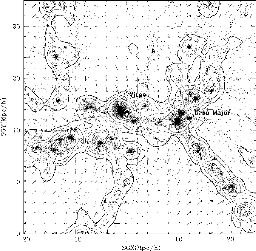
Figure 5: Density and velocity fields in the 45$h^{-1}$Mpc  region around the Virgo cluster. The velocities are in the Virgo cluster rest frame. The fields were smoothed with the Gaussian filter of 1.4$h^{-1}$Mpc  smoothing length. The circle at the origin of the coordinates marks the position of the Milky Way galaxy. Points show dark matter particles (10% of all particles is shown) in a slice of $10\mbox{$h^{-1}$Mpc}$ thickness centered on the Supergalactic plane ($SGZ=0$). Contours show the projected density in the slice: the thick contour corresponds to the average matter density of the Universe. The thin contours mark overdensities 2, 4, 6, and so on. The length of the thick arrow in the top right corner shows a velocity of $500~{}\rm km\ s^{-1}$.

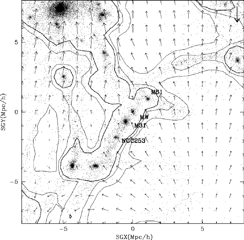
Figure 6: Density (contours) and velocity (arrows) fields (smoothed with a Gaussian filter of $0.7\mbox{$h^{-1}$Mpc}$ smoothing length) around the LG. The slice shown has a size and thickness of $15\mbox{$h^{-1}$Mpc}$ and $5\mbox{$h^{-1}$Mpc}$, respectively, and is centered on the supergalactic plane ($SGZ=0$). Points show positions of the dark matter particles (all particles are shown). Contours show the projected density in the slice: the thick contour corresponds to the overdensity 3; the other contours mark overdensities 1 and 2. The length of the thick arrow in the top right corner corresponds to a velocity of $500~{}\rm km\ s^{-1}$. The velocities are plotted in the Virgo cluster rest frame. Although the matter distribution bears some resemblance to the observed distribution of galaxies, observational data constraints on these scales are weak. Note the empty region to the right of the LG.

It is also clear that peculiar velocities do not exhibit a simple Virgocentric spherically symmetric infall pattern usually assumed in the models of the local velocity field (e.g., Aaronson et al., 1982; Huchra, 1988). Only in the immediate vicinity of the Virgo cluster (within $\sim 3$ Mpc of the cluster center) the velocity infall is Virgocentric and is close to being spherically symmetric. On larger scales the velocity flow is roughly perpendicular to the filament which constitutes the main body of the LSC, reflecting the fact that most of the mass is distributed in this filament rather than being concentrated in one cluster.

The predictions of the Virgocentric infall model fail to describe the properties of the simulated peculiar velocity field accurately both qualitatively and quantitatively. Figure 7 shows spherically averaged density, radial velocity, and velocity dispersion profiles centered on the Virgo cluster. The average density contrast at the distance of the LG in the simulation is $\delta\rho/\rho=0.69$. The dot-dashed line in Figure 7 shows the density model used by Huchra (1988) in the Virgocentric infall model: a constant density with added $r^{-2}$ law, which is normalized to have an overdensity of 4 at the LG distance. This model overpredicts the mass within the MW distance around the Virgo cluster in our simulation by a factor of three. This is consistent with the results of Villumsen & Davis (1986), Cen (1994), and Governato et al. (1997) who concluded that the Virgocentric infall model is quite inaccurate when tested using numerical simulations.

Figure 7 also shows that the average radial velocity of the dark matter is near zero within the virial radius of the Virgo cluster, which indicates that cluster matter is in virial equilibrium. The deviations of the average velocity from zero at larger radii shows that the matter near and just outside the virial radius is not fully relaxed. At even larger radii the profile shows the infall of unvirialized matter and can be well approximated as $145(13\mbox{$h^{-1}$Mpc}/r)^{1/2}~{}\rm km\ s^{-1}$ (shown by the dashed curve). The radial velocity dispersion profile in the top panel of Figure 7 is approximately flat at large radii (indicating the velocity dispersion typical in the LSC region), while within the virial radius the velocity dispersion profile has a shape typical for the halos formed in the CDM cosmologies (Navarro et al., 1997; Łokas & Mamon, 2001; Klypin et al., 1999).

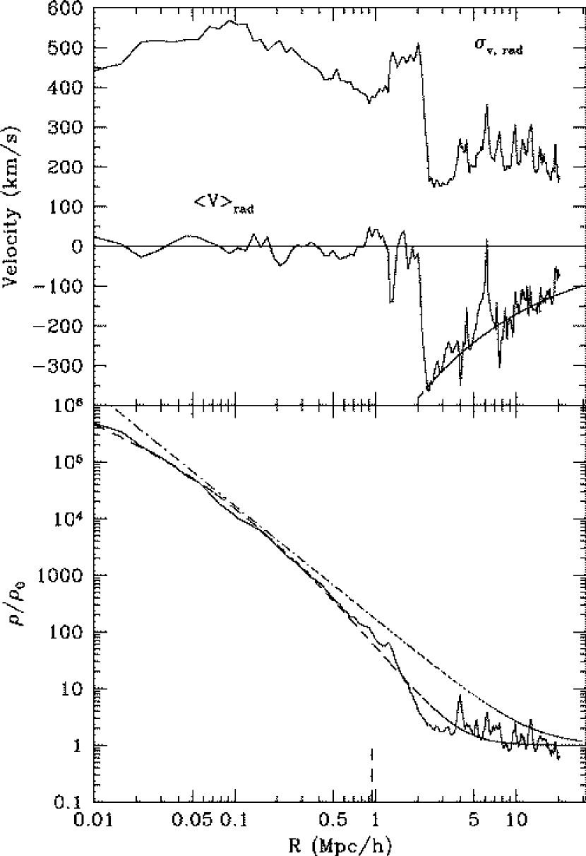
Figure 7: Spherically averaged profiles of density (bottom panel), average radial velocity (top panel, lower curve), and radial velocity dispersion (top panel, upper curve) constructed around the center of the Virgo cluster. Bottom panel: The density profile is shown in units of the average density of the universe, $\rho_{0}$. The short vertical dashed line on the x-axis at $\sim 1\mbox{$h^{-1}$Mpc}$ indicates the virial radius of the Virgo Cluster. The dashed curve shows the NFW profile (Navarro et al., 1997) with an added constant $\rho_{0}$ to account for the flattening of the profile at large radii. The dot-dashed curve shows the density model assumed by Huchra (1988) to model the velocity field in the LSC region. Top panel: note that the average radial velocity of the dark matter is very small within the virial radius of the Virgo cluster, which indicates an established virial equilibrium within the cluster. The dashed curve outside the virial radius shows a fit to the infall velocity profile outside the Virgo cluster: $145(13\mbox{$h^{-1}$Mpc}/r)^{1/2}~{}\rm km\ s^{-1}$.

Figure 8: The Hubble diagram (radial velocity as a function of radius) for halos in the simulation in the LG restframe. Individual halos are denoted by open circles with the circle radius representing the maximum circular velocity of the halo (larger circles correspond to more massive halos). The thick line shows the Hubble law, $v_{\rm H}=H_{0}r$, for the value $H_{0}=70{\ \rm km\ s^{-1}Mpc^{-1}}$ assumed in the simulation, and the thin lines correspond to velocities $v_{\rm H}\pm 100{\ \rm km\ s^{-1}}$. Note that deviations from the Hubble flow in the vicinity of the LG ($r\lesssim 7$$h^{-1}$Mpc) are $<100{\ \rm km\ s^{-1}}$ (i.e., the flow is “cold”).

Figure 8 shows the Hubble diagram for the simulated DM halos in the Milky Way restframe. Similarly to observations (e.g., Sandage, 1999), galactic halos follow the global Hubble expansion remarkably well. Note that deviations from the Hubble flow in the vicinity of the LG ($r\lesssim 7$$h^{-1}$Mpc) are $<100~{}\rm km\ s^{-1}$ and the flow is rather “cold”. In particular, similarly to the observed local Hubble flow (e.g., Giraud, 1986; Ekholm et al., 2001) only one halo (besides the M31 counterpart) has negative radial velocity (i.e., is blueshifted). Peculiar velocities increase at larger ($r\gtrsim 7$$h^{-1}$Mpc) radii due to the large concentration of mass in the main body of the LSC, in the immediate vicinity of the Virgo cluster. Table 1 presents the radial and 3-dimensional velocity dispersions in different radial shells around the MW for halo samples constructed using various selection criteria. The columns show the shell radius (1), radial velocity dispersion (2), 3-dimensional velocity dispersion (3), number of halos in the radial shell, halo sample selection criteria (5, with $N_{p}$ and $V_{\rm circ}$ denoting the number of particles per halo and the circular velocity of the halo, respectively). The rms radial velocity at $r=5\mbox{$h^{-1}$Mpc}$ is about $60~{}\rm km\ s^{-1}$ (virtually independent of the sample selection criteria) and increases to $\approx 110~{}\rm km\ s^{-1}$ at $r=10\mbox{$h^{-1}$Mpc}$.

To illustrate deviations from spherical symmetry in the velocity flow around the Virgo cluster, Figure 9 shows the peculiar radial velocities of DM particles along the line-of-sight passing through the the Virgo Cluster. All DM particles within $1.5\mbox{$h^{-1}$Mpc}$ around the line-of-sight are shown and particle velocities are computed in the restframe of the Virgo cluster. The most prominent feature in the radial velocity profile is the “finger of god” effect within the LG and the Virgo cluster. This well-known effect is due to large random velocities of particles within these massive halos. The LG and the Virgo cluster are the only massive systems along this line-of-sight. Therefore, the radial velocity dispersion of particles outside the virialized regions measure the “temperature” of the intergalactic velocity field. Note that the typical deviations from the coherent infall are very small on both sides of the Virgo Cluster: $\sim 50-60~{}\rm km\ s^{-1}$ at $r\lesssim 7\mbox{$h^{-1}$Mpc}$ and $\lesssim 10~{}\rm km\ s^{-1}$ at $r\gtrsim 18\mbox{$h^{-1}$Mpc}$, which reflects the relative “coldness” of the flow. The flow is especially cold at large radii because the matter at these radii undergoes a fairly uniform expansion out of a void.

The solid curve in Figure 9 represents a model for the infall velocity based on the Zeldovich approximation. The model was normalized to have the same infall velocity at the distance from the LG to the center of the Virgo cluster as found in the simulation. This model fares much better than the spherical Virgocentric infall model of Huchra (1988): it makes good fit for all velocities at all radii between the LG and the Virgo. Nevertheless, it failed because it required a mass between the LG and the Virgo that is about twice smaller than the corresponding mass in the simulation (compared to the factor of three overprediction of mass by the Virgocentric infall model). Moreover, the velocity flow on the other side of the Virgo cluster at $r\gtrsim 15\mbox{$h^{-1}$Mpc}$ is not reproduced by this model even qualitatively. In fact, the velocity flow around the Virgo cluster is clearly asymmetric and cannot be well described by a model with any kind of symmetry with respect to the Virgo cluster. This effort illustrates how difficult it is to construct a reasonable model for the velocity flow in the Local Supercluster.

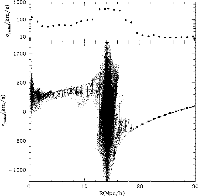
Figure 9: Bottom panel: Peculiar radial velocities of DM particles (points) along the line-of-sight from the LG through the center of the Virgo cluster. All particles within the radius of $1.5\mbox{$h^{-1}$Mpc}$ of the line-of-sight are plotted. Solid circles with error bars show average and the rms deviation of the radial velocities as a function of radius; the rms radial velocity dispersion is shown separately in the top panel. The Virgo Cluster is at the distance of $14\mbox{$h^{-1}$Mpc}$ from the LG. The particle velocities are computed in the restframe of the Virgo cluster.

Table 1: Peculiar velocity dispersions in the vicinity of the LG

Distance from the LG	$V_{\rm radial}$	$V_{\rm 3D}$	$N_{\rm halos}$	conditions
$h^{-1}$Mpc	$\rm km\ s^{-1}$	$\rm km\ s^{-1}$
5	$60\pm 16$	129	14	$N_{p}>10$ & $V_{\rm circ}>55~{}\rm km\ s^{-1}$
5	$58\pm 16$	130	13	$N_{p}>15$
5	$57\pm 16$	132	12	$N_{p}>20$ & $V_{\rm circ}>60~{}\rm km\ s^{-1}$
5	$48\pm 20$	136	6	$N_{p}>25$ & $V_{\rm circ}>90~{}\rm km\ s^{-1}$
6	$66\pm 14$	139	24	$N_{p}>15$
6	$67\pm 14$	141	17	$N_{p}>25$
8	$84\pm 13$	165	43	$N_{p}>15$
8	$77\pm 14$	181	29	$N_{p}>25$
10	$111\pm 13$	222	75	$N_{p}>15$
10	$110\pm 15$	222	55	$N_{p}>25$

6 Discussion and Conclusions

In the previous section we presented results of numerical simulations with initial conditions constructed using large-scale constraints from the observed density field (deduced using the MARK III peculiar velocity survey) and a random realization of the density field for the popular $\Lambda$CDM model of structure formation. These initial conditions lead to the formation of large-scale ($\gtrsim 5$$h^{-1}$Mpc) structures that match the observed structures within $\sim 100\mbox{$h^{-1}$Mpc}$ around the Local Group well, while the structures on smaller scales are not constrained and represent a random realization of the $\Lambda$CDM primordial power spectrum.

We show that such constrained simulations reproduce the most prominent nearby large-scale structures, such as the Coma cluster, the Great Attractor, the Perseus-Pisces supercluster, the LSC, and the Local Void. The locations of the structures varies within the ensemble of the constrained simulations (with different random realizations of the $\Lambda$CDM spectrum) by a few megaparsecs, but the overall qualitative large-scale morphology is reproduced robustly. The differences in structure location from realization to realization imply that the constrained simulations should not be expected to reproduce the observed structures accurately in the highly non-linear regime. Instead, they should be considered as a tool for generating realizations of the primordial density field for specific purposes and comparisons with observations in which it is crucial that the cosmic variance is greatly reduced. In other words, constrained simulations are well suited for studying the formation of particular objects, density field configurations, and environments. The outputs of constrained simulations can be used for generation of mock galaxy catalogs and testing empirical models (e.g., the peculiar velocity field models).

In this paper we used the constrained simulations (described in detail in § 3) to study the morphology of the density distribution and the peculiar velocity field in the $\sim 30\mbox{$h^{-1}$Mpc}$ region around the Virgo cluster (which we call the LSC region in this study). In particular, we focused on the question of the relative “coldness” of the peculiar velocity field in the immediate vicinity of the LG. We find that the velocity field in the LSC region is quite complex. Matter and halos in underdense regions, such as the Local Void, undergo coherent expansion as predicted by analytic models of void evolution (Hoffman & Shaham, 1982; Bertschinger, 1985). Near large-scale filaments and sheets the peculiar velocities are nearly perpendicular to the longest dimension of the closest structure, the pattern predicted by the Zel’dovich (1970) collapse solution.

The main body of the LSC (the $\sim 20\mbox{$h^{-1}$Mpc}$ filament centered on the Virgo cluster) in the simulation contains most of the mass in the LSC region ($\approx 7.5\times 10^{14}\mbox{$h^{-1}$Mpc}$), while the LG is located in an inconspicuous filament bordering the Local Void. The virial mass of the Virgo cluster is $\approx 1\times 10^{14}\mbox{$h^{-1}$Mpc}$ or less than 15% of the LSC mass and therefore the cluster does not dominate dynamics around the LSC. Correspondingly, a spherically symmetric Virgocentric infall model provides a very poor description of the peculiar velocity field which shows coherent infall in the overall direction of the extended mass concentration of the LSC rather than towards the Virgo cluster. In particular, the model overestimates the mass within $10\mbox{$h^{-1}$Mpc}$ around the Virgo cluster in our simulation by a factor of three. The value of matter density $\Omega_{0}$ inferred using this model is thus grossly inaccurate. This inaccuracy was pointed out in previous tests of this model in the LG like environments in cosmological simulations (Cen, 1994; Governato et al., 1997).

The matter within and around the LG counterpart in our simulation participates in the infall onto the LSC (roughly in the direction of the Virgo cluster) with a velocity of $\sim 250{\ \rm km\ s^{-1}}$. Although the observational measurements of the LG infall velocity span a wide range of values, the average value, $\sim 250\pm 50~{}\rm km\ s^{-1}$ (see, e.g., Huchra, 1988, and references therein), is in good agreement with that found in our simulation. The local overdensity of dark matter around the simulated LG is $\approx 5.5$ within $1.5\mbox{$h^{-1}$Mpc}$ and is about zero within $5\mbox{$h^{-1}$Mpc}$. This can be compared to the overdensity of galaxies of $\sim 0.25$ within $5\mbox{$h^{-1}$Mpc}$ in the IRAS survey (Schlegel et al., 1994). Given the small statistics and observational uncertainties this is a fair agreement: both the simulated and real LG appear to reside in only slightly overdense environments.

Although the LG is located in a filament, this filament is of relatively small mass and does not perturb the large-scale infall flow significantly. Therefore, the flow in the immediate vicinity of the LG is rather smooth. This explains the relative “coldness” of the local peculiar velocity field. The radial velocity dispersion within $\approx 7\mbox{$h^{-1}$Mpc}$ around the LG in the simulation is $\sim 40-70~{}\rm km\ s^{-1}$, which is in good agreement with observations (e.g., Sandage, 1986; Giraud, 1986; Schlegel et al., 1994; Karachentsev & Makarov, 1996; Ekholm et al., 2001, and references therein). The velocity dispersion increases to $\approx 110{\ \rm km\ s^{-1}}$ at larger distances due to larger peculiar velocities within and around the main body of the LSC.

The low value of the velocity dispersion we find in our simulation is in contrast with considerably higher values found for the simulated LG like systems in previous studies (Schlegel et al., 1994; Governato et al., 1997). We are not certain what caused the differences. We think that some of the differences are due to the different cosmological model. Very likely this is so in the case of the SCDM model as opposed to $\Lambda$CDM  model studied in this paper. In case of the open CDM model studied by Governato et al. (1997), which has the same density of matter as in our $\Lambda$CDM  model, the differences may also be partially attributed to a more accurate representation of the large-scale environment of the LG in our simulation. In any case, it is comforting that the “cold” local velocity field is reproduced within the current favored $\Lambda$CDM cosmological model and there is no need for exotic explanations (e.g., Chernin et al., 2001).

To conclude, we think that numerical experiments conducted under controlled conditions of constrained realizations should help to shed light on some of the unanswered questions in the theory of structure and galaxy formation. Some of these questions arise from the unique data in the immediate neighborhood of the LG. The observational constraints on the primordial density field can be strengthened with the improving size and accuracy of the peculiar velocity surveys. Indeed, even in the immediate future one can conceivably perform more accurate constrained simulations by combining the MARK III survey used in this study and the Surface Brightness Fluctuations (SBF; Tonry et al., 2001) peculiar velocity survey, which has more accurate velocities for nearby galaxies.

The question of the coldness of the local peculiar velocity field addressed in this paper is but a single example of the problems that can be addressed by constrained simulations. Indeed, in a related paper we extend the present work by using gas-dynamics constrained simulations to study properties of the intergalactic medium in the LSC region and formation of the Virgo cluster (Kravtsov et al., 2001). We also plan to use higher mass and force resolution constrained simulations to study the distribution of dwarf galaxies in the LSC and nearby voids, formation of the LG and other nearby groups and clusters, etc. Overall, we find that the constrained simulations provide an optimal tool for studying a wide range of dynamical problems concerning our “local” neighborhood within the large-scale structure of the Universe.

References

- Aaronson et al. (1982) Aaronson, M., Huchra, J., Mould, J., Schechter, P. L., & Tully, R. B. 1982, ApJ, 258, 64
- Bahcall & Joss (1976) Bahcall, J. N. & Joss, P. C. 1976, ApJ, 203, 23
- Bertschinger (1985) Bertschinger, E. 1985, ApJS, 58, 1
- Bertschinger (1987) —. 1987, ApJ, 323, L103
- Bistolas & Hoffman (1998) Bistolas, V. & Hoffman, Y. 1998, ApJ, 492, 439+
- Biviano (2001) Biviano, A. 2001, astro-ph/0010409
- Cen (1994) Cen, R. 1994, ApJ, 424, 22
- Chernin et al. (2001) Chernin, A., Teerikorpi, P., & Baryshev, Y. 2001, astro-ph/0012021
- Colín et al. (2000) Colín, P., Klypin, A. A., & Kravtsov, A. V. 2000, ApJ, 539, 561
- Davis et al. (1982) Davis, M., Huchra, J., Latham, D. W., & Tonry, J. 1982, ApJ, 253, 423
- Davis & Peebles (1983) Davis, M. & Peebles, P. J. E. 1983, ARA&A, 21, 109
- de Vaucouleurs (1953) de Vaucouleurs, G. 1953, AJ, 58, 30+
- de Vaucouleurs (1958) —. 1958, AJ, 63, 253+
- de Vaucouleurs (1976) —. 1976, ApJ, 203, 33
- de Vaucouleurs (1978) de Vaucouleurs, G. 1978, in IAU Symp. 79: Large Scale Structures in the Universe, Vol. 79, 205–212
- de Vaucouleurs (1989) —. 1989, The Observatory, 109, 237
- Einasto et al. (1984) Einasto, J., Klypin, A. A., Saar, E., & Shandarin, S. F. 1984, MNRAS, 206, 529
- Ekholm et al. (2001) Ekholm, T., Baryshev, Y., Teerikorpi, P., Hanski, M., & Paturel, G. 2001, accepted, astro-ph/0103090
- Fisher & Tully (1981) Fisher, J. R. & Tully, R. B. 1981, ApJS, 47, 139
- Gelb & Bertschinger (1994) Gelb, J. M. & Bertschinger, E. 1994, ApJ, 436, 491
- Giraud (1986) Giraud, E. 1986, A&A, 170, 1
- Governato et al. (1997) Governato, F., Moore, B., Cen, R., Stadel, J., Lake, G., & Quinn, T. 1997, New Astronomy, 2, 91
- Gunn (1978) Gunn, J. E. 1978, in Observational Cosmology Advanced Course, 1+
- Hoffman & Ribak (1991) Hoffman, Y. & Ribak, E. 1991, ApJ, 380, L5
- Hoffman & Ribak (1992) —. 1992, ApJ, 384, 448
- Hoffman & Shaham (1982) Hoffman, Y. & Shaham, J. 1982, ApJ, 262, L23
- Hoffman & Zaroubi (2000) Hoffman, Y. & Zaroubi, S. 2000, ApJ, 535, L5
- Huchra (1988) Huchra, J. P. 1988, in ASP Conf. Ser. 4: The Extragalactic Distance Scale, 257–280
- Huchra & Geller (1982) Huchra, J. P. & Geller, M. J. 1982, ApJ, 257, 423
- Karachentsev & Makarov (1996) Karachentsev, I. D. & Makarov, D. A. 1996, AJ, 111, 794+
- Klypin et al. (1999) Klypin, A., Gottlöber, S., Kravtsov, A. V., & Khokhlov, A. M. 1999, ApJ, 516, 530
- Klypin et al. (2001) Klypin, A. A., Kravtsov, A. V., Bullock, J. S., & P., P. J. 2001, in press, astro-ph/0006343
- Knebe et al. (2000) Knebe, A., Kravtsov, A. V., Gottlöber, S., & Klypin, A. A. 2000, MNRAS, 317, 630
- Kolatt et al. (1996) Kolatt, T., Dekel, A., Ganon, G., & Willick, J. A. 1996, ApJ, 458, 419+
- Kravtsov (1999) Kravtsov, A. V. 1999, PhD thesis, New Mexico State University
- Kravtsov et al. (2001) Kravtsov, A. V., Klypin, A. A., & Hoffman, Y. 2001, ApJ, 000, submitted
- Kravtsov et al. (1997) Kravtsov, A. V., Klypin, A. A., & Khokhlov, A. M. 1997, ApJS, 111, 73+
- Kudlicki et al. (2001) Kudlicki, A., Chodorowski, M., Strauss, M., & Ciecielag, P. 2001, submitted, astro-ph/0010364
- Lahav et al. (2000) Lahav, O., Santiago, B. X., Webster, A. M., Strauss, M. A., Davis, M., Dressler, A., & Huchra, J. P. 2000, MNRAS, 312, 166
- Lee et al. (1986) Lee, H., Hoffman, Y., & Ftaclas, C. 1986, ApJ, 304, L11
- Łokas & Mamon (2001) Łokas, E. L. & Mamon, G. A. 2001, MNRAS, 321, 155
- Lundmark (1927) Lundmark, K. 1927, Uppsala Medd., 30, 1+
- Navarro et al. (1997) Navarro, J. F., Frenk, C. S., & White, S. D. M. 1997, ApJ, 490, 493+
- Nolthenius et al. (1997) Nolthenius, R., Klypin, A. A., & Primack, J. R. 1997, ApJ, 480, 43+
- Peebles (1976) Peebles, P. J. E. 1976, ApJ, 205, 318
- Peebles (1992) Peebles, P. J. E. 1992, in Relativistic Astrophysics and Particle Cosmology, Texas/PASCOS 92 Symp., ed. C. W. Akerlof & M. A. Srednicki, Vol. 688 (Ann. NY Acad. Sci.), 84+
- Reynolds (1923) Reynolds, J. H. 1923, MNRAS, 83, 147+
- Rivolo & Yahil (1981) Rivolo, A. R. & Yahil, A. 1981, ApJ, 251, 477
- Sandage (1986) Sandage, A. 1986, ApJ, 307, 1
- Sandage (1999) —. 1999, ApJ, 527, 479
- Sandage & Tammann (1975) Sandage, A. & Tammann, G. A. 1975, ApJ, 196, 313
- Sandage & Tammann (1981) —. 1981, A revised Shapley-Ames Catalog of bright galaxies (Washington: Carnegie Institution, 1981, Preliminary version)
- Schlegel et al. (1994) Schlegel, D., Davis, M., Summers, F., & Holtzman, J. A. 1994, ApJ, 427, 527
- Shapley (1934) Shapley, H. 1934, MNRAS, 94, 791+
- Shaver (1991) Shaver, P. A. 1991, The space distribution of local radio galaxies, Tech. rep.
- Shaver & Pierre (1989) Shaver, P. A. & Pierre, M. 1989, A&A, 220, 35
- Silk (1974) Silk, J. 1974, ApJ, 193, 525
- Tonry et al. (2001) Tonry, J. L., Dressler, A., Blakeslee, J. P., Ajhar, E. A., Fletcher, A. ., Luppino, G. A., Metzger, M. R., & Moore, C. B. 2001, ApJ, 546, 681
- Tully (1982) Tully, R. B. 1982, ApJ, 257, 389
- Tully & Fisher (1987) Tully, R. B. & Fisher, J. R. 1987, Atlas of Nearby Galaxies (Annales de Geophysique)
- van de Weygaert & Hoffman (1999) van de Weygaert, R. & Hoffman, Y. 1999, in Evolution of Large Scale Structure : From Recombination to Garching, 178+
- van de Weygaert & Hoffman (2000) van de Weygaert, R. & Hoffman, Y. 2000, in ASP Conf. Ser. 201: Cosmic Flows Workshop, 169+
- Villumsen & Davis (1986) Villumsen, J. V. & Davis, M. 1986, ApJ, 308, 499
- Wang et al. (2001) Wang, X., Tegmark, M., & Zaldarriaga, M. 2001, submitted, astro-ph/0105091
- Willick et al. (1997) Willick, J. A., Courteau, S., Faber, S. M., Burstein, D., Dekel, A., & Strauss, M. A. 1997, ApJS, 109, 333+
- Yahil (1985) Yahil, A. 1985, in ESO Workshop on the Virgo Cluster, 359–373
- Yahil et al. (1980) Yahil, A., Sandage, A., & Tammann, G. A. 1980, ApJ, 242, 448
- Zaroubi (2001) Zaroubi, S. 2001, submitted, astro-ph/0010561
- Zaroubi et al. (1999) Zaroubi, S., Hoffman, Y., & Dekel, A. 1999, ApJ, 520, 413
- Zaroubi et al. (1995) Zaroubi, S., Hoffman, Y., Fisher, K. B., & Lahav, O. 1995, ApJ, 449, 446+
- Zaroubi et al. (1997) Zaroubi, S., Zehavi, I., Dekel, A., Hoffman, Y., & Kolatt, T. 1997, ApJ, 486, 21+
- Zel’dovich (1970) Zel’dovich, Y. B. 1970, A&A, 5, 84