HST photometry of globular clusters in the Sombrero galaxy

Abstract

We explore the rich globular cluster (GC) system of the nearby Sa galaxy M104, the “Sombrero” (NGC 4594), using archive WFPC2 data. The GC colour distribution is found to be bimodal at the $>99\%$ confidence level, with peaks at $(V-I)_{0}=0.96\pm 0.03$ and $1.21\pm 0.03$. The inferred metallicities are very similar to those of globular clusters in our Galaxy and M31. However the Sombrero reveals a much enhanced number of red (metal-rich) GCs compared to other well-studied spirals. Because the Sombrero is dominated by a huge bulge and only has a modest disk, we associate the two sub-populations with the halo and bulge components respectively. Thus our analysis supports the view that the metal-rich GCs in spirals are associated with the bulge rather than with the disk. The Sombrero GCs have typical effective (half-light) radii of $\sim$2 pc with the red ones being $\sim$30% smaller than blue ones. We identify many similarites between the Sombrero’s GC system and those of both late type spirals and early-type galaxies. Thus both the GC system and the Hubble type of the Sombrero galaxy appear to be intermediate in their nature.

1 Introduction

Observations with the Hubble Space Telescope have, in many ways, revolutionized our understanding of globular cluster systems (GCSs) in external galaxies. However, ellipticals and, to some extent, S0 galaxies have received by far the largest amount of attention, primarily because early-type galaxies tend to have much richer GCSs and suffer less from internal extinction problems than spirals. As a result, our knowledge of the GCSs in spiral galaxies is still limited to a handful of galaxies, including the Milky Way and M31.

Perhaps the most conspicuous difference between the GCSs of ellipticals and spirals is the much higher specific frequencies ($S_{N}=$ number of globular clusters per unit galaxy luminosity, Harris & van den Bergh 1981) of ellipticals. Spiral galaxies typically have $S_{N}\la 1$, while normal ellipticals have $S_{N}\sim 2-5$ and cDs often reach $S_{N}\sim 15$ [Harris 1991]. Part of this discrepancy may be removed if the $S_{N}$ of spirals is normalized only to the spheroidal component rather than to the total galaxy luminosity [Côté et al. 2000], although this approach becomes problematic for galaxies like the LMC and M33 which lack an obvious spheroidal component but do possess significant populations of globular clusters (e.g. Forbes et al. 2000). McLaughlin [McLaughlin 1999] has argued that the high specific frequencies of giant ellipticals may be explained if the number of globular clusters is instead normalised to the total galaxy mass, including hot X-ray emitting gas. In this way he finds a constant globular cluster formation efficiency with respect to the total initial gas mass available, but the remaining problem is then to explain why the field star formation efficency in the giant ellipticals is lower than that of GCs.

In addition to the Local Group galaxies, some of the best studied spirals are M81 and the two edge-on spirals NGC 4565 and NGC 5907. Although M81 is nearby, studies of its GCs are complicated by internal extinction in M81 and by its large angular size which causes confusion problems with foreground stars. However, available data indicate that the GCS of M81 is very similar to that of M31 and the Milky Way [Perelmuter & Racine 1995, Schroder et al. 2001]. In NGC 4565 and NGC 5907, internal extinction problems are minimized because of the edge-on orientation of these two galaxies. Again, the GCSs of these two galaxies (type Sb and Sc, respectively) appear to be quite similar to those of the Milky Way and M31 in terms of richness and spatial structure, with specific frequencies of $S_{N}\sim 0.5$ [Fleming et al. 1995, Kissler-Patig et al. 1999].

It has been known for many years that the Milky Way globulars can be divided into (at least) two populations, based on their metallicities and spatial distributions [Kinman 1959, Zinn 1985, Minniti 1995], where the metal-rich population appears to be associated with either the thick disk or the bulge component. Similar conclusions have been reached for the GCS of the Andromeda galaxy [Seitzer et al. 1996, Jablonka et al. 1998, Barmby et al. 2000]. In contrast, Kissler-Patig et al. [Kissler-Patig et al. 1999] suggested that, since NGC 4565 and NGC 5907 contain roughly equal numbers of globular clusters but have very different bulge to thin-disk and thick-disk to thin-disk ratios, these components of spiral galaxies may not have a significant influence on the building of globular cluster systems around such galaxies. However, metal-poor and metal-rich clusters were not addressed separately in the study of NGC 4565 and NGC 5907 and indeed the total numbers of GCs detected in these galaxies (40 and 25 respectively) were too small to permit such an analysis.

Within the last few years it has been firmly established that the GCSs of many, if not most, early-type galaxies also exhibit bimodal metallicity distributions [Gebhardt & Kissler-Patig 1999, Kundu & Whitmore 2001, Larsen et al. 2001]. The spatial distribution of red (metal-rich) clusters tends to be more centrally concentrated than that of the blue (metal-poor) ones. One of the more surprising results of recent HST imaging has been the discovery that the average sizes of metal-poor and metal-rich GCs in early-type galaxies differ by $\sim 30$%, with the metal-poor clusters being systematically larger [Kundu & Whitmore 1998, Kundu et al. 1999, Puzia et al. 1999, Larsen & Brodie 2000]. The sizes of globular clusters in the Milky Way also show a correlation with galactocentric distance, in the sense that clusters far from the centre are systematically larger [van den Bergh 1994]. This appears to be in contrast to the situation in elliptical galaxies, at least in NGC 4472 and M87 where no such trend is seen [Kundu et al. 1999, Puzia et al. 1999]. Furthermore, the size difference is apparently present over a large range of galactocentric distances [Larsen et al. 2001], so at least in some ellipticals it seems difficult to explain it as simply due to differences in the radial distributions of metal-rich and metal-poor globular clusters.

The “Sombrero” galaxy (M104 = NGC 4594) represents an important intermediate case between early-type galaxies and the Sb/Sc type spirals mentioned above. Although it clearly contains a star forming disk and a conspicuous dust lane, its integrated luminosity is dominated by a huge bulge/halo component. It is one of the nearest Sa–type galaxies, located at a distance of only 8.7 Mpc [Ford et al. 1996]. The first study of globular clusters in the Sombrero was carried out by Wakamatsu [Wakamatsu 1977] who identified a very rich GCS with an estimated total of about 2000 GCs. Harris et al. [Harris et al. 1984] identified $1200\pm 100$ globular clusters in the Sombrero, corresponding to a specific frequency of $3\pm 1$ with respect to the bulge/halo luminosity alone. A similar number of GCs was found by Bridges & Hanes [Bridges & Hanes 1992] who also estimated a mean metallicity of [Fe/H] = $-0.81\pm 0.05$ based on $B\!-\!V$ colours. This mean metallicity was confirmed spectroscopically by Bridges et al. [Bridges et al. 1997 1997] who obtained a mean [Fe/H] = $-0.70\pm 0.3$ for a sample of 34 GCs. Ground-based CCD imaging of the GCS by Forbes et al. [Forbes, Grillmair & Smith 1997] found some tentative evidence for two populations of GCs. However these results were uncertain due to contamination from foreground stars and background galaxies in their ground-based images. Two populations were confirmed by Gebhardt & Kissler-Patig [Gebhardt & Kissler-Patig 1999] in their study of 50 galaxies using archive WFPC2 data. However they did not comment on the Sombrero galaxy explicitly.

Here we present a new investigation of the globular cluster system of the Sombrero galaxy, using HST archive images of three fields.

Table 1: WFPC2 archive images of the Sombrero galaxy used in this paper.

Field	PID	PI	Filters	Exposures
Centre	5512	Faber	F547M $+$ F814W	$3\times 400+3\times 350$ s
Inner Halo	5091	Groth	F606W $+$ F814W	$800+800$ s
Outer Halo	5369	Griffiths	F606W $+$ F814W	$2\times 2100+2\times 2100$ s
Reference	7909	Casertano	F606W $+$ F814W	$500+400,500$ s

2 Data reduction

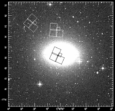
Figure 1: The three WFPC2 pointings on the Sombrero galaxy used for this study, superposed on an image from the Digitized Sky Survey.

Basic information about the datasets is listed in Table 1 and the pointings are illustrated in Fig. 1. The central pointing has the PC chip centred on the nucleus of the Sombrero galaxy and consists of $3\times 400$ s exposures in the F547M band and $3\times 350$ s in F814W. The WFPC2 field reaches out to a distance of about 4 kpc from the nucleus. The two halo pointings were both observed with the F606W and F814W filters and are located at $4\aas@@fstack{\prime}6$ (11 kpc projected) and $8\aas@@fstack{\prime}3$ (21 kpc projected) from the centre of the Sombrero. Unfortunately, only one exposure of 800 s in each filter was available for the inner halo pointing, which makes cosmic ray removal a more difficult task. For the outer pointing we use 2 exposures of 2100 s each in each filter, far deeper than the two other pointings. In addition, we use F606W and F814W data for a reference field at $227\arcmin$ from the Sombrero to estimate the number of foreground/background sources.

For the pointings where more than one exposure was available in each filter, the individual exposures in each band were combined into a single image using the IRAF task imcombine. For the central pointing, background subtraction was then performed by first removing point sources and then median filtering the resulting images as described in Larsen & Brodie [Larsen & Brodie 2000]. The median-filtered images were then subtracted from the original images.

The region around the dust lane and the high surface brightness areas near the nucleus were masked out before further analysis. Input object lists for photometry were then produced by running the daofind task in the daophot package within IRAF on both the $V$ and $I$ band images and matching the two resulting coordinate lists. As an additional selection criterion, the background noise was measured directly on the images in an annulus around each object and only objects with a S/N $>3$ in both $V$ and $I$ within an aperture radius of 2 pixels were accepted. In this way we accounted for the varying background noise, especially within the central pointing. For the inner halo pointing where the individual exposures suffered from quite substantial numbers of cosmic ray (CR) events, the object lists were inspected manually to make sure that all sources for which photometry was subsequently obtained would be real objects. The requirement that objects were detected both in $V$ and $I$ turned out to be quite efficient in eliminating CR hits from the object lists. However, a few GC candidates were manually removed from the object lists because of CR hits that would have affected the photometry.

The $V\!-\!I$ colours were measured through an $r=2$ pixels aperture using the phot task in daophot, while a larger $r=3$ pixels aperture was used for $V$ magnitudes to reduce systematic errors on the aperture corrections resulting from finite object sizes. The use of a smaller aperture for colours is justified because the $V$ and $I$ aperture corrections nearly cancel out when colour indices are formed [Holtzman et al. 1996, Larsen & Brodie 2000]. The photometry was transformed to standard $V,I$ magnitudes using the procedure in Holtzman et al. [Holtzman et al. 1995]. Globular clusters are expected to be resolved on HST images at the distance of M104 so we determined aperture corrections to the Holtzman et al. $r=0\aas@@fstack{\prime\prime}5$ reference aperture by convolving King profiles with the TinyTim PSF [Krist & Hook 1997] and carrying out aperture photometry on the resulting images. Because of the different image scales on the WF and PC chips, the aperture corrections will also be different. We found aperture corrections in $V$ of $-0.15$ mag and $-0.55$ mag for the WF and PC, respectively. These corrections assume clusters with effective (half-light) radii $\mbox{$R_{\rm eff}$}\sim 3$ pc. For larger clusters our magnitudes will be systematically too faint, by $\sim 0.2$ mag on the WF and $\sim 0.3$ mag on the PC chip if the cluster sizes are twice as large. For $V\!-\!I$ the aperture corrections are $0.030$ and $0.120$ mag for the WF and PC, changing by no more than $\sim 0.01$ mag for any reasonable cluster sizes. Finally, a correction for Galactic foreground extinction of $A_{V}=0.17$ mag [Schlegel et al. 1998] was applied to the photometry, corresponding to $E(V-I)=0.086$ [Cardelli, Clayton & Mathis 1989].

In addition to the photometry, we also measured sizes for individual objects in the HST images using the ishape algorithm [Larsen 1999a]. ishape convolves the PSF (in this case generated by TinyTim) with a series of different model profiles, adjusting the size (FWHM) of the model until the best possible match to the observed profile is obtained. In the case of HST images, ishape also convolves with the WFPC2 “diffusion kernel” [Krist & Hook 1997]. For the model profiles we adopted King [King 1962] profiles with a concentration parameter (ratio of tidal vs. core radius) of 30. Fitting the concentration parameter and linear size simultaneously would require better signal-to-noise and/or angular resolution than what is currently available for the Sombrero. However, as discussed in Larsen [Larsen 1999a], the effective radii derived from the ishape fits are not very sensitive to a particular choice of model profile as long as the sources have intrinsic sizes smaller than or comparable to that of the PSF.

3 Results

3.1 The central pointing

We first consider the data for the central pointing, as this is where the largest number of globular clusters was found.

Figure 2: Colour-magnitude diagram for objects in the WFPC2 chips on the central pointing. The dashed lines mark the boundary of the region within which globular cluster candidates were selected. Typical $V\!-\!I$ errors are indicated by the error bars.

Figure 3: Completeness functions for the WF frames (solid line) and PC frame (dashed line), determined from artificial object experiments.

Fig. 2 shows the reddening corrected colour-magnitude diagram for all objects detected in the central pointing down to $V=25$. The globular cluster sequence can be clearly seen, extending from $V\sim 20$ down to $V\sim 24$ and with $V\!-\!I$ colours between 0.8 and 1.4. Objects outside this colour range are expected to be mainly background sources. We selected globular cluster (GC) candidates as objects within the region marked by the dashed lines in Fig. 2, i.e. $0.75<\mbox{$(V\!-\!I)_{0}$}<1.45$ and $V<24$. This results in the identification of 151 GC candidates, listed in Table 2. If we convert the colour interval to a metallicity range using the calibration of Kissler-Patig et al. [Kissler-Patig et al. 1998], then it corresponds to $-2.05<\mbox{[Fe/H]}<+0.24$, but we note that these limits should only be taken as approximate since they are beyond the actual calibrated range.

Completeness tests for the photometry were carried out by adding artificial objects to the images and redoing the photometry to see how many of the artificial objects were recovered. Because the completeness functions will depend on object size, we generated the artificial objects by convolving the TinyTim PSF with King profiles with effective (half-light) radii of 3 pc. Since the GC candidates do not show a strong concentration towards the centre of the galaxy and we are masking out the regions near the dustlane, the artificial objects were simply distributed at random within each frame. The recovery fractions are shown as a function of magnitude in Fig. 3 for the WF (solid line) and PC frames (dashed line). From these tests we estimate the average 50% completeness level to be at $V\sim 24.5$ in the WF frames and at $V\sim 23.5$ in the PC frame. The brighter 50% limit in the PC frame is mainly due to the higher background level there. We thus reach well below the expected turn-over of the globular cluster luminosity function (GCLF) at $M_{V}\sim-7.5$ [Harris 1991], corresponding to $V\sim 22.4$.

The number of contaminating objects can be estimated from the comparison field. This field is located so far from the Sombrero galaxy ($227\arcmin\sim 575$ kpc) that no globular clusters are expected here. We find about 8 objects in this field resembling globular clusters by their colours and morphological appearance. Some of the objects in the comparison field are unresolved by ishape (presumably foreground stars) while others have apparent sizes comparable to globular clusters. The latter are most likely background galaxies.

3.1.1 Colour distribution

A glance at Fig. 2 suggests two peaks in the $(V\!-\!I)_{0}$ colour distribution. Applying a KMM test [Ashman, Bird & Zepf 1994] to the sample of GC candidates, we find that the colour distribution is bimodal at the 99.9% confidence level with peaks at $(V\!-\!I)_{0}$ = 0.96 and 1.21. These $V\!-\!I$ colours correspond to metallicities of [Fe/H] = $-1.4$ and [Fe/H] = $-0.54$ when using the relation of Kissler-Patig et al. [Kissler-Patig et al. 1998]. The KMM test itself does not provide error estimates for the peak colours but from experiments with different selection criteria for GC candidates we find that the peak colours are probably accurate to about $\pm 0.03$ mag, corresponding to $\pm 0.1$ in [Fe/H]. The KMM test assigns 45% of the GC candidates in the central pointing to the blue (metal-poor) peak and 55% to the red one.

Figure 4: Luminosity function for globular cluster candidates in the NGC 4594 central pointing. The solid line shows the best fitting $t_{5}$ function, $\mbox{${\rm M}^{\rm TO}_{V}$}=22.10$ and $\sigma_{t}=0.81$. Dashed lines: $t_{5}$ functions with the turn-over shifted by $\pm 0.15$ mag (the estimated $1\sigma$ error). Dotted-dashed line: $\sigma_{t}=0.91$.

3.1.2 Luminosity function

The luminosity function (LF) for GC candidates in the central pointing (corrected for Galactic foreground extinction) is shown in Fig. 4. The LF clearly has a peak at $V\sim 22$, although the histogram in Fig. 4 has more faint objects than would be expected for a “standard” Gaussian LF. The field around the Sombrero galaxy has many background galaxies and some of the faintest objects may be contaminants, but because the halo fields (see below) and the comparison field do not contain the same large numbers of faint objects within the GC colour range, part of the departure from a Gaussian LF may well be real. As noted e.g. by Secker [Secker 1992], there are other analytical functions which actually match the faint end of the GCLF in the Milky Way and M31 galaxies significantly better than a Gaussian, notably the ‘$t_{5}$’ function. The $t_{5}$ and Gaussian functions are hardly distinguishable above the turn-over, but for magnitudes fainter than the turnover a $t_{5}$ function has larger numbers of objects than a Gaussian.

We carried out $t_{5}$ function fits to the data in Fig. 4 using a maximum-likelihood algorithm. A correction for completeness was applied, using the completeness function derived from the artificial object tests, and contaminating objects were statistically subtracted from the GC sample using the comparison field. Objects in the PC frame were excluded from the fits because of the brighter completeness limit there. Fitting a $t_{5}$ function to all data in the WF chips down to $V=24$, we found a peak at $\mbox{${\rm m}^{\rm TO}_{V}$}=22.28\pm 0.12$ and a dispersion of $\sigma_{t}=1.02\pm 0.12$. Note that the dispersions of $t_{5}$ ($\sigma_{t}$) and Gaussian ($\sigma_{g}$) functions are related as $\sigma_{g}\approx 1.29\,\sigma_{t}$ [Secker 1992]. Applying a Kolmogorov-Smirnov (K-S) test (e.g. Lindgren 1962), the above fit is only accepted at the 82% confidence level, indicating that the $t_{5}$ function does not provide an incredibly good fit to the observed GCLF in the Sombrero over the full magnitude range. Without the completeness correction the peak would be at $\mbox{${\rm m}^{\rm TO}_{V}$}=22.22\pm 0.12$, while we get $\mbox{${\rm m}^{\rm TO}_{V}$}=22.46\pm 0.14$ if both the completeness and contamination corrections are omitted. Thus, the correction for incompleteness only has a small effect on the turn-over magnitude, while the contamination correction has a more pronounced effect.

If the fit is restricted to a narrower magnitude range then the effects of contamination, incompleteness and deviations from the assumed $t_{5}$ shape of the GCLF may be further reduced. If we adopt a magnitude limit of $V=23.5$ instead of 24.0 then the resulting $t_{5}$ fit has a turn-over at $\mbox{${\rm m}^{\rm TO}_{V}$}=22.05\pm 0.10$ and $\sigma_{t}=0.81\pm 0.10$, corresponding to a Gaussian $\sigma_{g}=1.05$. The K-S test now accepts the fit at the 99.8% confidence level, indicating no statistically significant deviations from a $t_{5}$ function for this brighter subsample. Leaving out the completeness correction has virtually no effect, changing ${\rm m}^{\rm TO}_{V}$ by only 0.01 mag to $22.04\pm 0.10$. This is not unexpected, considering that the applied magnitude limit is $\sim 1$ mag brighter than the 50% completeness limit. Again, the contamination correction has a stronger effect and without it the turn-over would be at $\mbox{${\rm m}^{\rm TO}_{V}$}=22.13\pm 0.12$. For an even brighter magnitude cut-off one expects the fits to become more uncertain as the sample size decreases and the dispersion becomes less well constrained, especially if the dispersion and turn-over are fitted simultaneously. Nevertheless, we find that the turn-over magnitude and dispersion of the $t_{5}$ function remain stable for a magnitude cut-off as bright as 22.0, even though the formal errors become larger. For cut-offs at $V=23.0$, 22.5 and 22.0 we find $\mbox{${\rm m}^{\rm TO}_{V}$}=22.10\pm 0.12$, $22.10\pm 0.18$ and $22.08\pm 0.24$, respectively.

Another possibility is to keep the dispersion fixed and only allow the turn-over to vary. If we adopt a fixed $\sigma_{t}=1.0$, corresponding to a Gaussian $\sigma_{G}=1.3$ (e.g. Kundu & Whitmore [Kundu & Whitmore 2001]) and perform a fit down to $V=23.5$ then we get a somewhat fainter turn-over at $\mbox{${\rm m}^{\rm TO}_{V}$}=22.15\pm 0.13$. However, the K-S test only accepts this fit at the 66% confidence level, indicating a much worse match to the data than for the two-parameter fit.

We thus adopt $\mbox{${\rm m}^{\rm TO}_{V}$}=22.10\pm 0.15$ as our best estimate of the reddening-corrected $V$-band turn-over magnitude for the GCLF of the Sombrero, where the $\pm 0.15$ uncertainty is based on the 1$\sigma$ errors returned by the maximum-likelihood fits as well as the scatter in the various fits. This corresponds to an absolute value of $\mbox{${\rm M}^{\rm TO}_{V}$}=-7.60\pm 0.15$ for a distance modulus of 29.7. For comparison, Secker [Secker 1992] found $\mbox{${\rm M}^{\rm TO}_{V}$}=-7.29\pm 0.13$ and $\mbox{${\rm M}^{\rm TO}_{V}$}=-7.51\pm 0.15$ for the Milky Way and M31. Note that the errors on these numbers are quite similar to our formal errors, consistent with the fact that a similar number of clusters are fitted. More recently, Barmby, Huchra and Brodie [Barmby, Huchra & Brodie 2001] found a $V$-band turn-over of $\mbox{${\rm m}^{\rm TO}_{V}$}=16.84$ for M31, or $\mbox{${\rm M}^{\rm TO}_{V}$}=-7.6$. Ferrarese et al. [Ferrarese et al. 2000] point out that a weighted mean to GCLF turn-over magnitudes for galaxies in the Virgo and Fornax gives $\mbox{${\rm M}^{\rm TO}_{V}$}=-7.60$ with a systematic difference of 0.5 mag between the two galaxy clusters. Kundu & Whitmore [Kundu & Whitmore 2001] favour a value of $\mbox{${\rm M}^{\rm TO}_{V}$}=-7.41$ based on a sample of 28 elliptical galaxies, but do not include any of the Fornax galaxies. Thus, our turn-over of $-7.60$ for the Sombrero may be somewhat on the bright side, but it is not clear how much of the scatter in reported turn-over magnitudes from various literature sources is intrinsic, and how much of it is due to different measurement techniques etc. The dispersion measured for the Sombrero GCLF ($\sigma_{t}=0.81\pm 0.10$ or $\sigma_{g}=1.05$) is formally somewhat narrower than the value in the Milky Way, but agrees well with the one in M31 ($\sigma_{g}$ = 1.42 and 1.06, respectively, Secker 1992).

Overall, we conclude that the GCLF of the Sombrero seems quite similar to that in most other well-studied galaxies. However, it is worth noting that the relatively small number of clusters does not provide very strong constraints on the exact form of the GCLF, a situation which can only be remedied by obtaining a larger sample of GCs.

Figure 5: Cluster half-light radii measured on the F547M images (central pointing) as a function of $(V\!-\!I)_{0}$ colour. The error bar indicates the typical random error on individual size measurements, as estimated in Sect 3.1.3.

Figure 6: Distributions of half-light radii for blue (top) and red (bottom) clusters in M104. On the average, blue clusters are larger than red ones. Hatched and outlined histograms are for sizes measured on F547M and F814W band images, respectively.

Figure 7: Comparison of object sizes for objects brighter than $V=23.5$, measured on F547M and M814W images. The solid line is a fit to the data points while the dashed line represents a 1:1 relation.

3.1.3 Globular cluster sizes

Fig. 5 shows cluster sizes as a function of $(V\!-\!I)_{0}$ colour. The sizes were measured by ishape on $V$ frames, excluding objects fainter than $V=23.5$ in order to avoid too low S/N objects where the size information would be uncertain.

As can be seen from the figure, the data for GCs in the Sombrero show a correlation between cluster size and $(V\!-\!I)_{0}$ colour similar to that in ellipticals and S0 galaxies [Kundu & Whitmore 1998, Puzia et al. 1999, Larsen et al. 2001]. The size difference between blue and red clusters (dividing at $\mbox{$(V\!-\!I)_{0}$}=1.05$) is seen somewhat more clearly in Fig. 6 where the size distributions for blue (top) and red (bottom) clusters are illustrated. In Fig. 6 the hatched and outlined histograms represent sizes measured on F547M and F814W band images, respectively. The sizes measured on the F814W images are generally somewhat larger (see below), but the size difference between red and blue GCs is clearly seen in both cases. The mean effective radii (defined as the radius within which half of the total cluster luminosity is contained) of red and blue clusters are $\mbox{$R_{\rm eff}$}=1.61$ pc and $\mbox{$R_{\rm eff}$}=2.09$ pc, measured on the F547M images.

We can also compare with cluster sizes measured on the PC frame. These should be more accurate, given the better resolution of the PC chip. For the 9 red and 9 blue cluster candidates on the PC chip with size information, the average sizes are 1.48 and 2.54 pc. Of course, small number statistics play a significant role here and the clusters near the nucleus might also have different physical sizes from those further out. In any case, the size difference between blue and red clusters is confirmed by both measurements.

The accuracy of the measured cluster sizes can be further checked by comparing size measurements on the F547M and F814W images. Fig. 7 compares sizes measured in the two bands for objects brighter than $V=23.5$, the same magnitude limit adopted for the cluster size measurements. The dashed line represents a 1:1 relation between the two sets of size measurements while the solid line is a least-squares fit to the data. As can be seen from the figure, the sizes measured on the F814W exposures are on the average $\sim 0.75$ pc larger than those measured on the F547M images. It is worth noting, though, that one WF camera pixel corresponds to a linear scale of 4.2 pc at the adopted distance of the Sombrero. The 0.75 pc offset could be due to small changes in the telescope focus (“breathing”), minor offsets between the combined exposures or inaccuracies in the PSF modelling by TinyTim. Until these effects are better understood, the absolute values of the sizes in Fig. 5 and Fig. 6 should not be taken too literally, but size differences are much more robust. Apart from the 0.75 pc offset, the two sets of size measurements agree quite well. The standard deviation around the fit indicated by the solid line in Fig. 7 is 0.7 pc, indicating that individual cluster sizes are accurate at about this level, not counting possible systematic effects.

3.2 The halo pointings

Figure 8: Colour-magnitude diagram for objects in the WFPC2 chips in the two halo pointings.

The colour-magnitude diagrams for the two halo fields are shown in Fig. 8. Obviously, the number of GC candidates in the halo fields are much smaller than in the central pointing, but these fields nevertheless serve as a very useful comparison. Using the same selection criteria as for the central field, the inner and outer halo fields contain 31 and 11 GC candidates, respectively (Table 2). While most of the objects in the inner halo field are probably true globular clusters, we expect a significant fraction of the objects in the outer halo field to be contaminants, bearing in mind that about 8 foreground/background objects are expected within the GC colour range.

The colour-magnitude diagrams in Fig. 8 are not quite as strikingly bimodal as the corresponding plot for the central field (Fig. 2), and bimodality is only detected at the 40% confidence level by a KMM test when combining data for the two halo pointings. Nevertheless, the peaks found by the KMM test are at $\mbox{$(V\!-\!I)_{0}$}=0.97$ and $\mbox{$(V\!-\!I)_{0}$}=1.19$, nearly identical to those in the central pointing. 60% of the objects in the halo pointings are assigned to the blue peak by the KMM test, compared to 45% in the central pointing, providing a hint that the ratio of blue (metal-poor) to red (metal-rich) clusters increases somewhat as a function of galactocentric distance.

3.3 Radial trends

Figure 9: GC sizes as a function of projected galactocentric distance in kpc. Plus ($+$) markers indicate red ($\mbox{$(V\!-\!I)_{0}$}>1.05$) clusters, diamonds ($\diamond$) blue clusters.

Figure 10: The surface density profile of the Sombrero GCS. The two outer points are for each of the halo pointings. The two lines represent analytical fits to an $R^{1/4}$ law and a power law as discussed in the text. One arcmin equals 2.5 kpc.

Data for all the three pointings have been combined to produce Fig. 9, which shows cluster sizes as a function of projected galactocentric distance $R_{\rm g}$. Red ($\mbox{$(V\!-\!I)_{0}$}>1.05$) and blue ($\mbox{$(V\!-\!I)_{0}$}<1.05$) clusters are shown with different symbols. We have not attempted to remove contaminants from Fig. 9. Although some of these will be foreground stars and thus appear point-like, others may be background objects with finite sizes that could be in the apparent GC size range. In addition to the contamination problem, observed radial trends in the cluster sizes may also be affected by the fact that the different exposures are taken through different passbands, with different exposure times and at different epochs. In particular, Holtzman et al. [Holtzman et al. 1999] noted that the HST point spread function can exhibit significant temporal variation due to the so-called “breathing” of the HST secondary mirror.

With these precautions in mind, the plot shows little, if any, correlation between cluster size and $R_{\rm g}$, at least for $R_{\rm g}\la 15$ kpc where most of the objects may still be expected to be globular clusters. Indeed, the average effective radii of objects in the three pointings are $1.77$, $1.99$ and $2.02$ pc for the central, inner and outer halo fields respectively.

The three HST pointings also allow us to investigate the radial density profile of the GCS as shown in Fig. 10. The central pointing has here been divided into three bins, plotting data for the PC chip separately and dividing the WF chip data at 3 kpc or about $1\aas@@fstack{\prime}2$. The two halo pointings each contribute with one data point. The total surface density of blue$+$red clusters is shown with error bars corresponding to Poisson statistics. We also plot data for red and blue clusters separately, although the error bars are omitted for clarity. The data in Fig. 10 have been corrected for foreground/background objects by subtracting 4 red and 4 blue objects from each pointing.

The azimuthal coverage of our data is clearly limited, but our four outermost data points for the surface density of globular clusters nevertheless agree quite well with results by Bridges & Hanes [Bridges & Hanes 1992] and with the GC counts quoted by Harris et al. [Harris et al. 1984]. The earlier ground-based studies were unable to probe the central few arcseconds of the Sombrero GCS, covered by the PC camera. It should, however, be pointed out that the PC data may still be uncertain because of possible obscuration from the dust lane which covers $\sim 50$% of the PC chip, even though we have attempted to mask out the most prominent parts of the dust lane.

We fitted the GC surface density $\sigma_{\rm GC}$ as a function of galactocentric radius $R_{g}$ with two different model profiles: A single power-law fit of the form

$$\sigma_{\rm GC}\propto R_{g}^{\alpha}$$ (1)

yields an exponent of $\alpha=-1.25\pm 0.20$, somewhat steeper than the value $-0.75\pm 0.15$ found by Bridges and Hanes [Bridges & Hanes 1992] for the central $4\arcmin$ but considerably shallower than the $-1.82$ value found by Harris et al. [Harris et al. 1984] for the outer regions. The actual profile is likely to be better represented as a composite of two power-laws [Bridges & Hanes 1992], although our relatively sparse coverage does not allow a more detailed investigation of this issue. However, the data do appear to be better fitted by a de Vaucouleurs $R^{1/4}$ profile of the form

$$\log\sigma_{\rm GC}=\alpha R_{g}^{1/4}+\beta$$ (2)

with $\alpha=-2.00\pm 0.18$ and $\beta=3.39\pm 0.23$. This is only slightly shallower than the value $\alpha=-2.12$ found by Harris et al. [Harris et al. 1984].

The total number of GCs in the Sombrero can be estimated by integration of (2). Adopting an outer radius of $20\arcmin$, we thus obtain a total of 1150 clusters which is nearly a factor of two smaller than the $\sim 2000$ GCs usually thought to exist in the Sombrero [Harris et al. 1984, Bridges & Hanes 1992, Forbes, Grillmair & Smith 1997]. However, the uncertainties on the fitted $\alpha$ and $\beta$ values translate to an uncertainty of about $\pm 50$% on the total number of clusters. The number of clusters also depends on the completeness correction, as well as on the adopted outer radius of the system. If this is taken to be $30\arcmin$ instead of $20\arcmin$ then the total number of GCs is $\sim 1290$. We have not corrected for incomplete sampling of the GC population due to the magnitude cut-off at V=24. Integrating a $t_{5}$ function with $\mbox{${\rm m}^{\rm TO}_{V}$}=22.1$ and $\sigma_{t}=0.81$ over the $V=19.0-24.0$ range, one finds that only about 4% of the globular clusters would fall outside this range. Alternatively, one can compare directly with the observed Milky Way GCLF: For a distance modulus of 29.7 our cut-off at $V=24$ corresponds to $M_{V}=-5.7$. Of the 144 GCs in the McMaster catalogue [Harris 1996] with tabulated $M_{V}$ values, 25 GCs or 17% fall below this limit. Thus, we estimate that we may have lost between 4% and 17% of the GCs in the Sombrero because of the magnitude limit.

The RC3 catalogue lists a total reddening-corrected $B$ magnitude of 8.38 and $\mbox{$(\mbox{$B\!-\!V$})_{0}$}=0.84$ for the Sombrero, leading to an absolute $V$ band magnitude of $M_{V}=-22.16$ for distance modulus 29.7. 1150 clusters then correspond to a specific frequency of $S_{N}=1.6\pm 0.8$ (where the $\pm 0.8$ comes from the $\pm 50$% estimated above), in reasonable agreement with earlier results but somewhat on the low side. Estimates of the bulge vs. total luminosity for the Sombrero range between 0.73 [Baggett, Baggett & Anderson 1998] and 0.85 [Kent 1988]. If we adopt 0.8 as a compromise, the bulge has $M_{V}=-21.92$ and the specific frequency with respect to the bulge alone becomes $S_{N}({\rm bulge})=2.0\pm 1.0$. If as many as 17% of the GCs are fainter than $V=24$ that would increase $S_{N}({\rm total})$ to around $1.9\pm 0.9$ and $S_{N}({\rm bulge})$ to $2.3\pm 1.2$.

If the red and blue cluster populations are fitted separately we obtain $\alpha_{R}=-2.07\pm 0.19$ and $\alpha_{B}=-1.91\pm 0.21$, again indicating that the spatial distribution of blue clusters is probably more extended than that of the red ones. The $\alpha$ values can be converted to effective radii (containing half the total number of clusters) for the de Vaucouleurs profiles, yielding $\mbox{$R_{\rm eff}$}_{,R}=6\aas@@fstack{\prime}7\pm 2\aas@@fstack{\prime}6$ and $\mbox{$R_{\rm eff}$}_{,B}=9\aas@@fstack{\prime}2\pm 3\aas@@fstack{\prime}9$ for the red and blue GCs respectively, assuming that the density profile continues to infinite radius. If we instead adopt an outer radius of $20\arcmin$ as above, which is probably a more reasonable assumption, then the respective effective radii become $\mbox{$R_{\rm eff}$}_{,R}=4\aas@@fstack{\prime}5\pm 1\aas@@fstack{\prime}0$ (11.4 kpc)and $\mbox{$R_{\rm eff}$}_{,B}=5\aas@@fstack{\prime}4\pm 1\aas@@fstack{\prime}1$ (13.7 kpc) for the red and blue GCs.

4 Discussion

We have clearly detected two sub-populations of GCs in the Sombrero galaxy, hinted at in Forbes et al. [Forbes, Grillmair & Smith 1997]. Thus, the Sombrero is like most large galaxies in this regard. The blue sub-population, with $(V-I)_{0}$ = 0.96 is quite similar in colour to the halo GCs in our Galaxy and M31, i.e. $\mbox{$(V\!-\!I)_{0}$}\sim 0.92$ [Barmby et al. 2000]. It is also remarkably similar to the mean value for a sample of early-type galaxies studied by Forbes & Forte [Forbes & Forte 2001], i.e. $(V-I)_{0}$ = 0.954 $\pm$ 0.008. The metallicity of [Fe/H] $=-1.4$ corresponding to the blue peak is also similar to that of metal-poor halo clusters in our Galaxy ([Fe/H] $=-1.59$) and M31 ([Fe/H] $=-1.40$) [Forbes et al. 2000]. It is therefore likely that the blue GCs in all these systems are old and metal–poor.

The red GCs have $(V-I)_{0}$ = 1.21 or [Fe/H] $=-0.54$. This is very similar to the metallicities of the “metal-rich” sub-population in both our Galaxy and M31, i.e. [Fe/H] $=-0.55$ and $-0.58$ respectively [Forbes et al. 2000]. So again, by analogy with known spirals, we associate the red GCs in the Sombrero with a bulge/disk population.

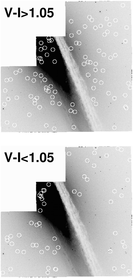
Figure 11: Spatial distributions of red (top) and blue (bottom) clusters. The dust lane and the brightest parts of the disk were masked out before photometry, so the absence of objects near the disk is not real. The apparent peculiar alignment of blue objects in the PC frame is probably just a consequence of the small number of detections in this chip.

The relation between host galaxy luminosity and the colours of globular cluster subpopulations has been studied in a number of recent papers. Forbes et al. [Forbes, Brodie & Grillmair 1997] found a correlation between host galaxy luminosity and the colour/metallicity of the red GCs, but no significant trend with luminosity for the blue GCs. More recently, Larsen et al. [Larsen et al. 2001] found correlations at the $2-3\sigma$ level with host galaxy luminosity for the colours of both GC populations. Kundu & Whitmore [Kundu & Whitmore 2001] and Burgarella, Kissler-Patig & Buat [Burgarella, Kissler-Patig & Buat 2001] found at best weak correlations between host galaxy luminosity and GC colours, while Forbes & Forte [Forbes & Forte 2001] detected a correlation between the colour of the red GCs and host galaxy central velocity dispersion, but no correlation for the blue GCs. The Sombrero does not represent an outlier with respect to any of the above datasets and was, in fact, included in the samples studied by both Larsen et al. [Larsen et al. 2001] and Burgarella, Kissler-Patig & Buat [Burgarella, Kissler-Patig & Buat 2001]. Note, however, that the mean colours of the two GC populations quoted here are slightly different from those in Larsen et al. [Larsen et al. 2001] (0.939 and 1.184 instead of the 0.96 and 1.21 values in this paper), even though the two studies use the same dataset. This difference reflects the slightly different colour / magnitude cuts adopted in the two analyses, but is within our estimated $\pm 0.03$ mag error margins. In fact, with the GC colours in the present paper the Sombrero fits even better onto the Larsen et al. [Larsen et al. 2001] relation for galaxy luminosity vs. GC colour.

In spiral galaxies the blue GCs are naturally associated with a halo population. In our Galaxy, the metal-poor halo GCs are distributed nearly spherically around the galaxy centre while the metal-rich population has a somewhat flattened distribution [Kinman 1959, Zinn 1980]. The spatial distributions of red and blue clusters in the central Sombrero pointing are shown in Fig. 11. From this figure it seems that the spatial distributions of red and blue GCs are not strikingly different within the central $\sim 4$ kpc covered by the archive images, but the spatial distribution of the red GCs is clearly different from the stellar disk of the Sombrero. The limited spatial coverage of WFPC2 makes it difficult to draw firm conclusions regarding any differences in the distributions of red and blue clusters further out. However, there are some indications that the number of blue clusters declines more slowly as a function of distance from the centre, implying that the ratio of blue to red clusters increases outward.

An interesting difference between the Sombrero GC system and that of other spiral galaxies is the relatively low ratio of metal-poor (blue) to metal-rich (red) GCs, i.e. about 0.8:1 in the central pointing and perhaps slightly higher for the GCS as a whole. Using metallicities and galactocentric radii for GCs in the Milky Way from the McMaster catalogue [Harris 1996] and dividing between metal-rich and metal-poor clusters at [Fe/H] $=-1.0$, the corresponding ratio within the central 4 kpc of our own Galaxy is $\sim 1.2:1$. In M31 it is $\sim 1.0:1$, using data from Barmby et al. [Barmby et al. 2000]. Further out in the halo of spiral galaxies metal-poor clusters dominate, leading to global blue-to-red ratios of about 2:1 and 3:1 in the Milky Way and M31 respectively. For early type galaxies the ratio is almost always $>$1:1 although red GCs also here tend to be more centrally concentrated than blue ones [Forbes, Brodie & Grillmair 1997].

Given that the stellar bulge-to-disk ratio for Sombrero is 6:1 [Kent 1988] and that the overall ratio of metal-poor to metal-rich globular clusters is much lower than in spiral galaxies with less conspicuous bulges, it seems very unlikely that the red GCs are associated with the disk but must rather be associated with the bulge. If the red GCs were associated with the disk we might expect a number roughly similar to that in the Milky Way, i.e. about 50 or so. In Section 3.3 we estimated a total number of around 1150 GCs in the Sombrero so if there are roughly equal numbers of red and blue GCs then that would imply a total of $\sim 600$ red GCs. Thus the situation in the Sombrero lends support to the idea that the metal-rich GCs also in our own and other spiral galaxies are more closely associated with the bulge than the disk [Harris 1976, Frenk & White 1982, Minniti 1995].

Another similarity between the Sombrero and other spirals, as well as early-type galaxies, is the relationship between GC colour and physical size. Here we find that the blue GCs are $\sim$30% larger than the red ones. This is seen in several early type galaxies and also in the Milky Way [Larsen et al. 2001]. It is not currently clear what causes this difference, which could be either set up at formation e.g. because of different conditions in the globular cluster progenitor clouds, or due to ongoing dynamical processes. As noted above, the blue GC population does appear to be more spatially extended than the red, but the current data are too sparse to study radial trends in the cluster sizes in detail and e.g. check how the GC sizes correlate with galactocentric distance. It is also possible that the different GC populations are on different orbits, in which case dynamical destruction processes might also affect them in different ways.

5 Concluding Remarks

Using HST imaging of the central few kpc of the nearby Sombrero galaxy we have detected $\sim$150 globular cluster candidates. We find a bimodal GC colour distribution with peaks at $\mbox{$(V\!-\!I)_{0}$}=0.96$ and 1.21, corresponding to [Fe/H] = $-1.4$ and $-0.54$ [Kissler-Patig et al. 1998]. The blue GCs have a mean size of 2.09 and the reds 1.61 pc. Including additional data for two halo pointings at projected distances of 11 kpc and 21 kpc from the nucleus of the Sombrero, we have studied radial trends in cluster sizes and the relative numbers of red and blue clusters. We find that the red clusters appear to be more centrally concentrated in the galaxy than the blue ones, although it would be highly desirable to confirm this result with better sample statistics. As an Sa galaxy, the Sombrero offers a potential link between the GC systems of elliptical galaxies and later type spirals. Indeed we find several similarities between the GC system of the Sombrero and galaxies of all types.

$\bullet$ The blue GCs have a mean colour (and hence metallicity) that is similar to those seen both in large spirals and ellipticals.

$\bullet$ The size-colour relationship is qualitatively the same as that seen in the Milky Way and several well-observed ellipticals.

$\bullet$ The red GCs have an inferred metallicity that is very close to the metal-rich populations of the Milky Way and M31 and other large galaxies.

$\bullet$ Without corrections for incomplete sampling of the GCLF, the GC specific frequency normalised to the total galaxy luminosity is $S_{N}({\rm total})=1.6\pm 0.8$, or $S_{N}({\rm bulge})=2.0\pm 1.0$ when normalised to the bulge. Corrections for incomplete sampling would increase these numbers by between 4% and 17%. The specific frequency of the Sombrero is thus similar to that of field and group ellipticals.

$\bullet$ The large number of red GCs compared to other spirals, combined with the high bulge/disk ratio in the Sombrero and the spatial distribution of the red GCs, suggests that this GC sub-population is associated with the bulge (rather than the disk) component.

The proximity and rich GC system of the Sombrero galaxy clearly warrant further study. Better HST coverage beyond the central few kpc would improve sample statistics and size/colour trends with galactocentric radius could be better probed. Spectra with $8-10$ m class telescopes would provide direct metallicity and age estimates for individual GCs. Kinematics of the two subpopulations could also be explored.

6 Acknowledgements

This work was supported by National Science Foundation grant number AST9900732, Faculty Research funds from the University of California, Santa Cruz and NATO Collaborative Research grant CRG 971552. We are grateful to Carl Grillmair and an anonymous referee for their useful comments. DF thanks the hospitality of Lick Observatory where much of this work was carried out.

Table 2: Data for clusters in the Sombrero. $V$ and $(V\!-\!I)_{0}$ have been corrected for a foreground extinction of $A_{V}=0.17$ and $E(V-I)=0.086$ mag. The last column is the estimated effective (half-light) cluster radius in pc. Note that sizes for objects fainter than $V=23.5$ (in parentheses) are uncertain. Prefixes ‘C’, ‘H1’ and ‘H2’ denote objects in the central, outer and inner halo pointings, respectively.

ID	RA(2000.0)	DEC(2000.0)	$V$	$(V\!-\!I)_{0}$	$R_{\rm eff}$
C-001	12:40:00.31	-11:37:21.4	19.22	1.28	1.78
C-002	12:39:59.40	-11:37:25.2	20.88	1.15	1.55
C-003	12:39:58.69	-11:37:28.2	21.53	1.08	1.05
C-004	12:39:58.65	-11:37:25.8	20.18	1.34	1.05
C-005	12:39:58.52	-11:37:25.9	22.85	0.90	1.92
C-006	12:39:58.45	-11:37:26.5	20.70	1.17	1.46
C-007	12:39:59.58	-11:37:16.7	21.21	1.07	1.22
C-008	12:39:59.02	-11:37:17.8	20.14	1.09	3.06
C-009	12:39:58.81	-11:37:18.7	22.54	1.04	3.50
C-010	12:39:59.76	-11:37:11.8	21.47	0.95	1.69
C-011	12:39:58.77	-11:37:17.6	20.11	1.03	2.54
C-012	12:39:59.33	-11:37:12.0	20.96	0.98	1.60
C-013	12:39:59.92	-11:37:07.7	23.31	1.27	0.06
C-014	12:39:58.55	-11:37:16.4	21.52	1.17	1.72
C-015	12:39:59.15	-11:37:12.3	22.45	0.95	3.00
C-016	12:39:58.92	-11:37:13.6	20.79	0.89	4.75
C-017	12:39:59.00	-11:37:13.0	23.08	1.26	1.34
C-018	12:39:59.66	-11:37:08.4	23.80	1.11	(err)
C-019	12:40:00.12	-11:37:04.6	22.25	1.02	2.62
C-020	12:39:59.01	-11:37:11.1	21.96	0.78	1.22
C-021	12:39:59.58	-11:37:06.9	23.22	1.19	0.52
C-022	12:39:59.85	-11:36:41.3	22.58	1.24	3.69
C-023	12:39:59.86	-11:36:36.0	23.92	1.39	(2.01)
C-024	12:40:00.59	-11:36:55.4	21.70	1.24	err
C-025	12:40:00.59	-11:36:55.4	21.70	1.24	1.49
C-026	12:40:00.88	-11:37:00.6	22.60	1.31	0.84
C-027	12:40:00.73	-11:36:49.6	21.02	0.98	1.36
C-028	12:40:00.63	-11:36:45.3	20.83	1.10	1.81
C-029	12:40:01.02	-11:36:57.5	21.94	1.01	1.62
C-030	12:40:00.18	-11:36:27.4	22.73	1.25	1.10
C-031	12:40:01.30	-11:37:02.4	23.58	1.19	(2.85)
C-032	12:40:01.05	-11:36:54.1	20.38	0.97	1.49
C-033	12:40:00.10	-11:36:23.0	22.60	1.25	1.30
C-034	12:40:01.00	-11:36:50.8	22.32	1.15	1.36
C-035	12:40:01.96	-11:37:05.5	21.70	1.24	0.78
C-036	12:40:01.90	-11:37:00.0	22.99	1.13	3.69
C-037	12:40:02.06	-11:36:59.3	21.92	1.20	1.62
C-038	12:40:01.22	-11:36:31.0	23.87	0.83	(1.17)
C-039	12:40:00.79	-11:36:16.4	22.22	1.22	1.56
C-040	12:40:01.02	-11:36:21.9	22.74	1.03	2.92
C-041	12:40:02.24	-11:37:00.8	22.55	1.35	1.94
C-042	12:40:02.49	-11:37:07.3	21.19	1.26	1.10
C-043	12:40:01.01	-11:36:17.3	22.34	0.88	5.70
C-044	12:40:02.60	-11:37:05.9	21.37	1.00	1.68
C-045	12:40:01.19	-11:36:16.3	21.32	0.94	2.14
C-046	12:40:02.03	-11:36:40.2	23.44	1.25	5.31
C-047	12:40:02.77	-11:37:02.0	22.65	1.11	3.95
C-048	12:40:01.68	-11:36:24.9	22.64	1.42	11.66
C-049	12:40:02.34	-11:36:45.6	23.69	1.28	(0.78)
C-050	12:40:01.60	-11:36:19.5	22.51	0.90	0.78
C-051	12:40:01.51	-11:36:15.5	21.17	1.18	1.62
C-052	12:40:02.37	-11:36:40.5	23.33	0.97	0.13
C-053	12:40:02.48	-11:36:44.0	21.46	0.91	3.37
C-054	12:40:02.43	-11:36:42.3	22.83	1.26	0.91
C-055	12:40:03.35	-11:37:05.2	23.06	1.00	1.81
C-056	12:40:03.19	-11:36:59.4	23.83	1.34	(6.16)
C-057	12:40:03.04	-11:36:53.9	23.45	1.00	err
C-058	12:40:03.04	-11:36:53.9	23.45	0.99	1.04
C-059	12:40:02.65	-11:36:40.9	21.14	1.17	0.97
C-060	12:40:03.48	-11:37:06.0	22.06	1.20	4.86

Table 2 (continued)
C-061 12:40:01.74 -11:36:09.2 22.18 1.08 1.17 C-062 12:40:02.32 -11:36:21.6 21.11 0.95 0.45 C-063 12:40:03.15 -11:36:46.1 23.90 1.02 (0.32) C-064 12:40:02.58 -11:36:27.7 21.10 0.94 1.43 C-065 12:40:03.58 -11:36:59.3 23.65 1.04 (1.04) C-066 12:40:03.10 -11:36:44.0 22.67 1.07 1.88 C-067 12:40:03.30 -11:36:29.7 22.19 1.22 1.56 C-068 12:40:03.13 -11:36:03.1 20.37 1.11 2.20 C-069 12:40:04.51 -11:36:45.3 23.57 0.87 (1.68) C-070 12:40:04.81 -11:36:52.1 21.35 0.92 2.27 C-071 12:40:03.36 -11:36:05.9 23.95 0.81 (10.89) C-072 12:40:04.85 -11:36:52.4 21.85 0.99 2.72 C-073 12:40:03.56 -11:36:09.5 23.56 1.22 (0.84) C-074 12:40:04.61 -11:36:42.1 21.56 1.06 2.20 C-075 12:40:04.82 -11:36:42.4 20.91 0.90 2.20 C-076 12:40:03.39 -11:35:56.0 21.36 0.90 2.79 C-077 12:40:05.09 -11:36:48.7 21.42 1.20 0.91 C-078 12:40:04.34 -11:37:14.4 22.21 1.18 0.58 C-079 12:40:03.96 -11:37:19.1 19.88 1.12 3.37 C-080 12:40:05.61 -11:37:09.6 22.66 1.39 0.78 C-081 12:40:04.55 -11:37:18.1 21.73 1.14 1.62 C-082 12:40:02.34 -11:37:49.4 23.10 1.28 0.32 C-083 12:40:04.27 -11:37:43.2 23.52 1.38 (0.97) C-084 12:40:03.45 -11:37:48.8 23.07 1.10 1.81 C-085 12:40:02.98 -11:37:53.8 22.75 1.10 1.17 C-086 12:40:02.21 -11:37:59.4 19.57 1.27 2.46 C-087 12:40:04.66 -11:37:43.5 22.43 1.13 2.01 C-088 12:40:03.32 -11:37:59.1 23.31 1.33 0.39 C-089 12:40:02.51 -11:38:06.8 23.23 1.09 1.62 C-090 12:40:04.30 -11:38:01.7 22.52 1.14 0.71 C-091 12:40:05.30 -11:37:57.1 22.16 0.96 1.49 C-092 12:40:06.66 -11:37:53.0 21.41 0.95 1.81 C-093 12:40:06.95 -11:37:51.1 20.93 1.21 0.78 C-094 12:40:04.85 -11:38:05.4 20.21 1.05 1.30 C-095 12:40:04.15 -11:38:11.1 21.56 1.05 0.65 C-096 12:40:05.03 -11:38:14.7 21.92 0.93 1.23 C-097 12:40:06.80 -11:38:03.2 23.39 0.81 2.79 C-098 12:40:05.42 -11:38:14.3 23.04 0.99 3.11 C-099 12:40:04.97 -11:38:17.8 23.95 1.12 (0.58) C-100 12:40:05.82 -11:38:12.5 22.43 1.22 0.52 C-101 12:40:05.93 -11:38:12.9 22.32 1.31 err C-102 12:40:04.23 -11:38:26.9 22.16 1.30 1.17 C-103 12:40:07.33 -11:38:06.7 22.69 0.84 0.91 C-104 12:40:04.60 -11:38:26.7 21.50 1.23 0.78 C-105 12:40:01.80 -11:38:02.5 21.88 1.32 1.56 C-106 12:40:01.42 -11:37:50.3 23.85 1.15 (0.19) C-107 12:40:01.52 -11:37:57.6 22.12 1.21 1.49 C-108 12:40:01.41 -11:37:55.5 22.47 1.12 2.85 C-109 12:40:01.83 -11:38:20.8 22.30 1.26 2.33 C-110 12:40:00.98 -11:37:55.2 20.16 1.23 1.17 C-111 12:40:01.76 -11:38:21.6 21.36 0.96 1.68 C-112 12:40:01.81 -11:38:26.9 22.11 1.10 1.43 C-113 12:40:01.42 -11:38:15.3 22.04 1.13 2.27 C-114 12:40:00.96 -11:38:12.3 21.87 1.10 1.49 C-115 12:40:01.66 -11:38:35.6 23.48 1.03 12.96 C-116 12:40:00.22 -11:37:53.0 19.98 0.96 2.07 C-117 12:39:59.90 -11:37:44.5 22.24 1.22 1.10 C-118 12:40:01.12 -11:38:30.5 23.14 0.95 3.11 C-119 12:39:59.85 -11:37:49.0 22.02 0.96 1.17 C-120 12:39:59.80 -11:37:55.4 21.98 1.23 1.49

Table 2 (continued)
C-121 12:39:59.68 -11:37:52.4 22.20 1.17 1.04 C-122 12:40:01.13 -11:38:44.0 21.03 1.15 2.98 C-123 12:40:00.74 -11:38:49.5 21.49 0.88 1.62 C-124 12:39:58.99 -11:37:51.2 23.34 1.18 err C-125 12:39:59.99 -11:38:25.7 21.78 1.18 1.62 C-126 12:40:00.33 -11:38:37.5 23.93 1.18 (12.96) C-127 12:39:59.40 -11:38:08.0 21.69 0.98 4.34 C-128 12:39:59.00 -11:38:00.4 23.79 1.13 (err) C-129 12:39:59.88 -11:38:30.0 22.53 1.11 1.88 C-130 12:39:59.09 -11:38:06.5 22.81 0.98 0.71 C-131 12:40:00.19 -11:38:51.9 21.26 1.26 1.04 C-132 12:39:59.21 -11:38:19.5 20.91 1.15 1.04 C-133 12:39:58.78 -11:38:09.5 22.43 1.35 0.84 C-134 12:39:59.25 -11:38:25.8 20.29 1.24 1.04 C-135 12:39:59.43 -11:38:35.8 21.18 1.22 1.30 C-136 12:39:57.97 -11:37:57.7 21.53 1.06 1.49 C-137 12:39:59.33 -11:38:43.8 21.10 1.19 1.30 C-138 12:39:58.63 -11:38:21.7 23.85 0.84 (15.55) C-139 12:39:58.63 -11:38:21.7 23.85 0.84 (err) C-140 12:39:58.54 -11:38:19.6 21.68 1.14 1.94 C-141 12:39:58.94 -11:38:35.6 21.99 1.16 1.30 C-142 12:39:58.26 -11:38:18.5 21.14 1.08 1.36 C-143 12:39:58.05 -11:38:17.2 23.51 0.96 (2.92) C-144 12:39:59.38 -11:39:01.5 21.03 0.92 2.20 C-145 12:39:58.31 -11:38:39.5 20.09 0.89 2.40 C-146 12:39:56.98 -11:38:01.7 21.68 0.98 1.56 C-147 12:39:57.72 -11:38:28.3 22.34 0.84 4.28 C-148 12:39:58.48 -11:38:58.7 22.60 1.08 1.36 C-149 12:39:58.37 -11:38:57.6 21.89 1.00 3.11 C-150 12:39:58.16 -11:38:54.6 22.11 0.84 2.27 C-151 12:39:57.39 -11:38:32.1 19.41 0.90 16.33

Table 2 (continued)
H1-01 12:40:20.67 -11:31:09.2 23.62 1.13 (3.65) H1-02 12:40:20.31 -11:31:12.3 22.32 1.18 5.31 H1-03 12:40:20.11 -11:30:26.5 21.94 1.35 0.65 H1-04 12:40:21.98 -11:30:07.4 22.54 0.89 6.03 H1-05 12:40:25.72 -11:30:60.0 21.78 1.00 2.59 H1-06 12:40:23.62 -11:31:40.4 23.29 1.07 6.35 H1-07 12:40:25.23 -11:32:03.3 23.29 0.86 14.71 H1-08 12:40:28.03 -11:31:43.5 21.25 0.86 0.06 H1-09 12:40:23.88 -11:32:37.2 23.04 1.23 0.45 H1-10 12:40:19.21 -11:32:07.0 22.46 0.97 2.72 H1-11 12:40:20.67 -11:32:49.9 22.21 0.93 0.26 H2-01 12:40:01.31 -11:32:17.5 21.67 1.13 2.83 H2-02 12:40:02.74 -11:31:57.5 23.91 1.23 (0.45) H2-03 12:40:02.91 -11:32:12.8 23.84 1.18 (23.33) H2-04 12:40:03.43 -11:32:23.1 23.42 0.95 2.98 H2-05 12:40:04.24 -11:32:21.1 21.71 1.20 1.56 H2-06 12:40:04.49 -11:31:59.1 20.28 0.92 0.32 H2-07 12:40:04.49 -11:31:57.8 22.04 1.41 0.06 H2-08 12:40:04.93 -11:32:02.2 22.88 1.13 7.45 H2-09 12:40:05.55 -11:32:31.7 20.45 0.97 2.33 H2-10 12:40:06.01 -11:32:15.7 20.51 1.01 0.19 H2-11 12:40:06.15 -11:32:30.2 23.74 0.78 (0.52) H2-12 12:40:06.40 -11:32:38.9 21.85 0.82 0.06 H2-13 12:40:06.75 -11:32:26.9 21.24 1.35 0.71 H2-14 12:40:03.55 -11:33:10.8 22.76 0.99 1.23 H2-15 12:40:07.53 -11:33:10.0 22.02 0.80 0.06 H2-16 12:40:05.53 -11:33:18.0 23.97 0.92 (8.49) H2-17 12:40:06.14 -11:33:21.3 22.40 0.97 0.84 H2-18 12:40:07.24 -11:33:26.2 22.49 1.07 3.63 H2-19 12:40:03.00 -11:33:30.6 22.19 0.97 1.04 H2-20 12:40:06.34 -11:33:29.9 21.44 1.06 0.97 H2-21 12:40:04.39 -11:33:36.1 23.75 0.99 (17.50) H2-22 12:40:02.07 -11:33:16.2 19.13 1.23 0.71 H2-23 12:40:01.21 -11:33:12.6 22.68 1.03 9.53 H2-24 12:40:01.02 -11:33:35.9 23.76 1.16 (3.37) H2-25 12:40:00.51 -11:33:04.9 23.80 1.12 (err) H2-26 12:40:00.45 -11:34:02.7 22.87 1.12 2.98 H2-27 12:40:00.09 -11:34:05.8 22.04 1.14 3.43 H2-28 12:39:59.79 -11:33:00.5 23.90 1.13 (8.81) H2-29 12:39:58.63 -11:33:13.7 22.64 1.06 2.07 H2-30 12:39:58.04 -11:33:19.4 21.14 0.96 2.01 H2-31 12:39:57.88 -11:33:55.0 21.13 0.84 0.39

References

- [Ashman, Bird & Zepf 1994] Ashman K. M., Bird C. M., Zepf S. E., 1994, AJ, 108, 2348
- [Baggett, Baggett & Anderson 1998] Baggett W. E., Baggett S. M., Anderson K. S. J., 1998, AJ, 116, 1626
- [Barmby et al. 2000] Barmby P., Huchra J. P., Brodie J. P., et al., 2000, AJ, 119, 727
- [Barmby, Huchra & Brodie 2001] Barmby P., Huchra J. P., Brodie J. P., 2001, AJ, 121, 1482
- [Bridges & Hanes 1992] Bridges T. J., Hanes D. A., 1992, AJ, 103, 800
- [Bridges et al. 1997 1997] Bridges T. J., et al., 1997, MNRAS, 284, 376
- [Burgarella, Kissler-Patig & Buat 2001] Burgarella D., Kissler-Patig M., Buat V., 2001, AJ, 121, 2647
- [Cardelli, Clayton & Mathis 1989] Cardelli J. A., Clayton G. C., Mathis J. S., 1989, ApJ, 345, 245
- [Côté et al. 2000] Côté P., Marzke R. O., West M. J., Minniti D., 2000, ApJ, 533, 869
- [Ferrarese et al. 2000] Ferrarese L., Mould J. R., Kennicutt R. C., et al., 2000, ApJ, 529, 745
- [Fleming et al. 1995] Fleming D. E. B., Harris W. E., Pritchet C. J., Hanes D. A., 1995, AJ, 109, 1044
- [Forbes, Grillmair & Smith 1997] Forbes D. A., Grillmair C. J., Smith R. C., 1997, AJ, 113, 1648
- [Forbes, Brodie & Grillmair 1997] Forbes D. A., Brodie J. P., Grillmair C. J., 1997, AJ, 113, 1652
- [Forbes et al. 2000] Forbes D. A., Masters, K. L., Minniti, D., Barmby, P., 2000, A&A, 358, 471
- [Forbes & Forte 2001] Forbes D. A., Forte, J. C., 2001, MNRAS, 322, 257
- [Ford et al. 1996] Ford H. C., Hui X., Ciardullo R., Jacoby G. H., Freeman K. C., 1996, ApJ, 458, 455
- [Frenk & White 1982] Frenk C. S., White S. D. M., 1982, MNRAS, 198, 173
- [Gebhardt & Kissler-Patig 1999] Gebhardt K., Kissler-Patig M., 1999, AJ, 118, 1526
- [Harris 1976] Harris W. E., 1976, AJ, 81, 1095
- [Harris & van den Bergh 1981] Harris W. E., van den Bergh, S., 1981, AJ, 86, 1627
- [Harris et al. 1984] Harris W. E., Harris H. C., Harris G. L. H., 1984, AJ, 89, 216
- [Harris 1991] Harris W. E., 1991, ARA&A, 29, 543
- [Harris 1996] Harris W. E., 1996, AJ, 112, 1487
- [Holtzman et al. 1995] Holtzman J. A., Burrows C. J., Casertano S., Hester J. J., Trauger J. T., Watson A. M., Worthey G., 1995, PASP, 107, 1065
- [Holtzman et al. 1996] Holtzman J. A., Watson A. M., Mould J. R., et al. 1996, AJ, 112, 416
- [Holtzman et al. 1999] Holtzman J. A., Gallagher J. S. III, Cole, A. A. et al. 1999, AJ, 118, 2262
- [Jablonka et al. 1998] Jablonka P., Bica E., Bonnatto C., et al., 1998, A&A, 335, 867
- [Kent 1988] Kent, S. M., 1988, AJ, 96, 514
- [King 1962] King, I. R., 1962, AJ, 67, 471
- [Kinman 1959] Kinman T. D., 1959, MNRAS, 119, 538
- [Kissler-Patig et al. 1998] Kissler-Patig M., Brodie J. P., Schroder L. et al., 1998, AJ, 115, 105
- [Kissler-Patig et al. 1999] Kissler-Patig M., Ashman K. M., Zepf S. E., Freeman K. C., AJ, 118, 197
- [Krist & Hook 1997] Krist J., Hook R., 1997, “The Tiny Tim User’s Guide”, STScI
- [Kundu & Whitmore 1998] Kundu A., Whitmore B. C., 1998, AJ, 116, 2841
- [Kundu et al. 1999] Kundu A., Whitmore B. C., Sparks W. B. et al., 1999, AJ, 513, 733
- [Kundu & Whitmore 2001] Kundu A., Whitmore B. C., 2001, AJ, 121, 2950
- [Larsen 1999a] Larsen S. S., 1999, A&AS, 139, 393
- [Larsen & Brodie 2000] Larsen S. S., Brodie J., 2000, AJ, 120, 2938
- [Larsen et al. 2001] Larsen S. S., Brodie J. P., Huchra J. P., Forbes D. A., Grillmair C. J., 2001, AJ, 121, 2974
- [Lindgren 1962] Lindgren, B. W. 1962, “Statistical Theory”, Macmillan Company, New York
- [McLaughlin 1999] McLaughlin D. E., 1999, AJ, 117, 2398
- [Minniti 1995] Minniti D., 1995, AJ, 109, 1663
- [Perelmuter & Racine 1995] Perelmuter J.-M., Racine R., 1995, AJ, 109, 1055
- [Puzia et al. 1999] Puzia T. H., Kissler-Patig M., Brodie J. P., Huchra J. P., 1999, AJ, 118, 2734
- [Schlegel et al. 1998] Schlegel D. J., Finkbeiner D. P., Davis, M., 1998, ApJ, 500, 525
- [Schroder et al. 2001] Schroder L., Brodie, J. P., Huchra, J. P. et al., 2001, AJ, accepted
- [Secker 1992] Secker J., 1992, AJ, 104, 1472
- [Seitzer et al. 1996] Seitzer P., Banas K. R., Armandroff T., 1996, BAAS 189.7117
- [van den Bergh 1994] van den Bergh S., 1994, AJ, 108, 2145
- [Wakamatsu 1977] Wakamatsu, K-I., 1977, PASP, 89, 267
- [Zinn 1980] Zinn R., 1980, ApJ, 241, 602
- [Zinn 1985] Zinn R., 1985, ApJ, 293, 424