Modelling the orbital modulation of ultraviolet resonance lines in high-mass X-ray binaries

The stellar-wind structure in high-mass X-ray binaries (HMXBs) is investigated through modelling of their ultraviolet (UV) resonance lines. For the OB supergiants in two systems, Vela X-1 and 4U1700$-$37, high-resolution UV spectra are available; for Cyg X-1, SMC X-1, and LMC X-4 low-resolution spectra are used. In order to account for the non-monotonic velocity structure of the stellar wind, a modified version of the Sobolev Exact Integration (SEI) method by Lamers et al. (1987) is applied.
The orbital modulation of the UV resonance lines provides information on the size of the Strömgren zone surrounding the X-ray source. The amplitude of the observed orbital modulation (known as the Hatchett-McCray effect), however, also depends on the density- and velocity structure of the ambient wind. Model profiles are presented that illustrate the effect on the appearance of the HM effect by varying stellar-wind parameters. The $q$ parameter of Hatchett & McCray (1977), as well as other parameters describing the supergiant’s wind structure, are derived for the 5 systems. The X-ray luminosity needed to create the observed size of the Strömgren zone is consistent with the observed X-ray flux. The derived wind parameters are compared to those determined in single OB supergiants of similar spectral type.
Our models naturally explain the observed absence of the HM effect in 4U1700$-$37. The orbital modulation in Vela X-1 indicates that besides the Strömgren zone other structures are present in the stellar wind (such as a photo-ionization wake). The ratio of the wind velocity and the escape velocity is found to be lower in OB supergiants in HMXBs than in single OB supergiants of the same effective temperature.

1 Introduction

In a high-mass X-ray binary (HMXB) a massive, early-type star transfers mass onto a compact companion, a neutron star or a black hole. The potential energy associated with the accreted matter is efficiently converted into X-rays (Davidson & Ostriker 1973). The mass transfer can take place in two different ways: (i) via the massive star’s dense stellar wind which is partly intercepted by the strong gravitational field of the compact companion; or (ii) via a flow of matter towards the compact star through the inner Lagrangian point (Roche-lobe overflow). In the latter case an accretion disk is expected to be present in the system, as well as a rapidly spinning X-ray source. The massive star is either an OB supergiant with a dense radiation-driven wind or a Be-type star characterised by strong H$\alpha$ emission arising from a slowly outflowing, dense equatorial disk. For reviews on this subject we refer to Lewin et al. (1995), van Paradijs (1998) and Kaper (2001).

The accretion-induced X-ray luminosity gives a direct measure of the wind density and velocity at the orbit of the X-ray source. In this sense, the compact object acts as a probe in the stellar wind. In OB-supergiant systems, the X-ray source strongly affects the supergiant’s radiation-driven wind. The X-ray source ionizes the surrounding wind regions creating an extended (Strömgren) zone of strong ionization that trails the X-ray source in its orbit. This causes the orbital modulation of ultraviolet (UV) resonance lines (Hatchett & McCray 1977; Kaper et al. 1993). Hatchett & McCray predicted this effect to be observable in UV resonance lines of the HMXB HD153919/4U1700$-$37. The HM-effect has, however, not been detected in spectra obtained with the International Ultraviolet Explorer (IUE), as shown by Dupree et al. (1978). Although Hammerschlag-Hensberge et al. (1990) reported variations with orbital phase in some subordinate lines, Kaper et al. (1990) reported that these variations are caused by variable Raman-scattered emission lines and are not due to the HM-effect (see also Kaper et al. 1993).

Table 1: System parameters of the HMXBs in our sample. References are: a) Walborn (1973); b) Chevalier & Ilovaisky (1977); c) Webster et al. (1972); d) Conti (1978); e) Bregman et al. (1973); f) Osmer (1973); g) Sadakane et al. (1985); h) Heap & Corcoran (1992); i) Bolton (1975); j) Levine et al. (1991); k) Rappaport & Joss (1983); l) Nagase (1989); m) Kemp (1977); n) van Paradijs & Kuiper (1984); o) Deeter et al. (1987); p) Haberl et al. (1989); q) Bolton & Herbst (1976); r) Kaper (1998).

X-ray companion			Optical primary
Name	$M_{\rm X}/M$⊙	$L_{\rm X}$(erg/s)r	Name	spec.type	$m_{\rm V}$	$M_{\rm\star}/M_{\odot}$	$R_{\rm\star}/R_{\odot}$	$a/R_{\odot}$	$P_{\rm orb}$(d)	$d$(kpc)
Cyg X-1	13i	$1.3\times 10^{37}$	HDE226868	O9.7 Iaba	8.87e	21i	18i	43i	5.60000m	1.8d
LMC X-4	1.38j	$2.2\times 10^{38}$	Sk-Ph	O8 V-IIIb	14b	14.7j	7.6j	12j	1.40839j	50
SMC X-1	1.05k	$2.6\times 10^{38}$	Sk 160	B0 Ibc	13.2f	17.0k	16.5k	25 k	3.89239n	60
Vela X-1	1.77l	$4.6\times 10^{36}$	HD77581	B0.5 Iabd	6.88g	23.0l	34.0l	52.9l	8.964416o	1.9g
4U1700$-$37	1.8h	$9.8\times 10^{35}$	HD153919	O6.5 Iaf+a	6.51h	52h	18h	36h	3.411652p	1.7q

Dupree et al. (1980) did detect the HM-effect in IUE spectra of HD77581/Vela X-1. The B-supergiant’s wind profiles are less saturated while the Strömgren zone is expected to be larger than in the case of HD153919/4U1700$-$37. A detailed study of the orbital modulation of the UV resonance lines of HD77581/Vela X-1 indicated that the velocity and density structure of the stellar wind cannot be a monotonically rising function with distance from the star (Kaper et al. 1993), a conclusion that has been derived from observations of single early-type stars as well (Lucy 1982). Additional absorption (e.g. due to material trailing the X-ray source in its orbit) appears in the line profiles at late orbital phases (Sadakane et al. 1985; Kaper et al. 1994).

HD153919 and HD77581 are the only OB-supergiants in HMXBs bright enough in the UV to have been observed with sufficient signal-to-noise in the high-resolution mode of IUE. Kallman et al. (1987) and Payne & Coe (1987) studied the HD77581/Vela X-1 system in low-resolution mode and trailing mode, respectively, to search for the signature of rapid modulation of the Strömgren zone as a reaction to the periodically varying X-ray emission from the pulsar. Although these early experiments with IUE were unsuccessful, the periodic modulation was recently detected using the Faint Object Spectrograph onboard the Hubble Space Telescope (HST) by Boroson et al. (1996). Treves et al. (1980) detected the orbital modulation of UV resonance lines in low-resolution IUE spectra of HD226868/Cyg X-1. This source is too faint to obtain useful high-resolution IUE spectra (Davis & Hartmann 1983). Bonnet-Bidaud et al. (1981) and van der Klis et al. (1982) discussed the appearance of the HM-effect in low-resolution IUE spectra of Sk 160/SMC X-1 and Sk-Ph/LMC X-4. Two high-resolution UV spectra of Sk 160/SMC X-1 confirmed the orbital modulation of the Si iv resonance doublet (Hammerschlag-Hensberge et al. 1984). Vrtilek et al. (1997) and Boroson et al. (1999) discussed observations of LMC X-4, including high-resolution HST/GHRS spectra, in terms of a shadow wind. In this system the X-ray flux is so strong that only in the X-ray shadow behind the supergiant companion a normal stellar wind can develop (Blondin 1994). This represents the most extreme case of the HM effect; in practice, only Roche-lobe overflow systems will include a shadow wind. Recent HST/STIS observations by Kaper et al. (in preparation) confirm the presence of a shadow wind in LMC X-4, as well as a photo-ionization wake at the (leading) interface between the shadow wind and the X-ray ionization zone. We have not included the peculiar O7 III/black-hole candidate system #32/LMC X-1 (Hutchings et al. 1983, 1987; Cowley et al. 1995) because the system is embedded in a nebula with strong (UV) emission lines.

Although detailed observational studies of the HM effect in individual systems exist, a quantitative analysis based on state-of-the-art stellar-wind models is lacking. In the past two decades significant improvement has been made in modelling the stellar-wind profiles of (single) OB-type stars (Groenewegen et al. 1989; Groenewegen & Lamers 1989, 1991; Haser et al. 1998). We present a quantitative analysis of the UV spectral variability in the five HMXBs with OB-supergiant companion observed with IUE, comparing the complete set of IUE spectra. The model spectra are obtained using a modified version of the Sobolev Exact Integration (SEI) method introduced by Lamers et al. (1987). Our new method allows to take into account the non-monotonic wind structure observed in many (single) OB-type stars by adding “turbulence”, as well as an extended Strömgren zone around the X-ray source. With this analysis, fundamental parameters of the system are derived.

An overview of the data and spectral line variability is given in Sect. 2. X-ray eclipse spectra, UV continuum lightcurves and additional photometry are described in Appendices A–C, and the applied variability and error analysis method is described in Appendix D. Sect. 3 introduces the radiation transfer code “SEI” (Lamers et al. 1987) and the modifications that we implemented to be able to compute line profiles for HMXBs. Sect. 4 describes our attempts to model the UV line variability observed in HD77581/Vela X-1 and HD153919/4U1700$-$37. The derived terminal velocities, ionization fractions and sizes of the ionization zones are discussed in Sect. 5.

2 IUE observations of High-Mass X-ray Binaries

Table 2: SWP number, Reduced Julian Day (RJD) = JD$-$2 440 000 and mid-exposure orbital phase $\phi$ of the IUE spectra. Spectra used to construct $\phi\sim 0$ and $\phi\sim 0.5$ averages are indicated by a suffix $\circ$ and $+$, respectively. Orbital parameters:

HDE226868/Cyg X-1			$\phi_{0}\equiv$ RJD 2804.245				P=$5{\aas@@fstack{d}}60000(24)$			(Kemp 1977)
Sk 160/SMC X-1			$\phi_{0}\equiv$ RJD 3000.1626(8)				P=$3{\aas@@fstack{d}}89239(2)$			(van Paradijs & Kuiper 1984)
Sk-Ph/LMC X-4			$\phi_{0}\equiv$ RJD 7742.4904(2)				P=$1{\aas@@fstack{d}}40839(1)$			(Levine et al. 1991)
HD77581/Vela X-1			$\phi_{0}\equiv$ RJD 4279.0466(37)				P=$8{\aas@@fstack{d}}964416(49)$			(Deeter et al. 1987)
HD153919/4U1700$-$37			$\phi_{0}\equiv$ RJD 6161.3400(30)				P=$3{\aas@@fstack{d}}411652(26)$			(Haberl et al. 1989)
SWP	RJD	$\phi$	1968	3699	0.775	21569	5656	0.728	22324	5752	0.407	4753	3958	0.2124
Cyg X-1			2020∘	3705	0.221	21607	5660	0.888	32961+	7214	0.432	5180	4003	0.3758
1273∘	3599	0.929	2044∘	3708	0.906	21608∘	5660	0.019	32967+	7215	0.543	25586	6160	0.7770
1445	3629	0.317	6203∘	4102	0.185	21609∘	5660	0.066	33085+	7233	0.550	25587	6160	0.7884
1451+	3629	0.441	6207+	4103	0.406	21611	5661	0.166	46144	8933	0.165	25588	6160	0.8020
1478∘	3632	0.971	6219+	4104	0.705	21612	5661	0.217	46151	8934	0.278	25589	6160	0.8169
1500+	3636	0.540	6224∘	4105	0.949	21613	5661	0.267	46167	8935	0.406	25590	6160	0.8299
1515∘	3638	0.047	7092	4182	0.826	21614	5661	0.315	4U1700$-$37			25591	6160	0.8423
1979	3701	0.270	7094	4182	0.878	21615	5661	0.360	1476	3632	0.7960	25592	6160	0.8545
2049+	3708	0.538	8662∘	4334	0.850	21616	5661	0.408	1714∘	3664	0.0093	25596∘	6161	0.0976
3012	3799	0.714	8673	4335	0.130	21617	5661	0.454	1960	3700	0.6277	25597	6161	0.1074
3079	3802	0.257	8687	4336	0.396	21618+	5661	0.494	1961	3700	0.6393	25598	6161	0.1228
3107	3804	0.640	8701	4337	0.617	21619+	5661	0.534	1969	3701	0.8508	25599	6161	0.1371
3518∘	3845	0.024	LMC X-4			21625∘	5662	0.003	1970	3701	0.8669	25600	6161	0.1462
3535	3848	0.388	1477∘	3632	0.950	Vela X-1			1972	3701	0.9098	25607	6162	0.3640
3940	3892	0.281	2045	3708	0.587	1442+	3628	0.453	1973∘	3701	0.9241	25608	6162	0.3746
3965	3894	0.732	6202	4102	0.368	1488∘	3634	0.057	1975∘	3701	0.9619	25609	6162	0.3844
3966	3894	0.744	6204+	4102	0.505	2087	3712	0.856	1986	3702	0.2536	25610	6162	0.3954
5178∘	4002	0.049	6208	4103	0.115	3510	3845	0.604	1987	3702	0.2740	25611	6162	0.4068
5181	4003	0.084	6220∘	4104	0.945	3519	3846	0.714	1991	3703	0.4572	25612	6162	0.4174
5183	4003	0.110	6223+	4105	0.482	3550	3850	0.140	1992+	3703	0.4716	25613	6162	0.4279
5475	4035	0.780	6225	4105	0.609	3649+	3862	0.537	1994+	3703	0.5038	25614	6162	0.4377
7784	4265	0.953	6226	4105	0.660	4718	3954	0.770	1995	3703	0.5186	25615	6162	0.4550
9340	4412	0.169	7066	4179	0.508	18823+	5323	0.457	2002	3703	0.6092	25616	6162	0.4658
9364	4416	0.834	7091	4182	0.454	18958+	5341	0.529	2003	3703	0.6357	25617+	6162	0.4778
9394	4419	0.395	8663	4334	0.396	18970	5343	0.743	2004	3703	0.6540	25618+	6163	0.4880
9397	4419	0.491	8664+	4334	0.446	18983∘	5345	0.976	2006	3704	0.7411	25619+	6163	0.4996
9413	4422	0.940	8674	4335	0.175	19012	5351	0.609	2008	3704	0.7672	25620+	6163	0.5295
9421	4423	0.117	8675	4335	0.221	19061	5357	0.282	2009	3704	0.7818	25621+	6163	0.5413
9439	4425	0.474	8686	4336	0.802	22278	5746	0.733	2106∘	3715	0.0384	28730	6632	0.1508
9459	4426	0.767	8688	4336	0.896	22287	5747	0.845	2153	3720	0.4570	28731	6632	0.1638
SMC X-1			8689	4336	0.937	22297∘	5748	0.975	4742∘	3957	0.9378	28732	6632	0.1775
1520+	3639	0.361	9366	4416	0.372	22301∘	5749	0.068	4751	3958	0.1839
1533∘	3642	0.930	21472	5646	0.585	22309	5751	0.290	4752	3958	0.1978

Our sample comprises five HMXBs; only for HD77581/Vela X-1 and HD153919/4U1700$-$37 high-resolution IUE spectra will be discussed. The system parameters (Table 1) are collected from the literature. Vela X-1 is an X-ray pulsar, identifying the compact object as a neutron star. For 4U1700$-$37 no X-ray pulsations have been detected, but the X-ray spectrum suggests that the X-ray source is a neutron star (White & Marshall 1983; Reynolds et al. 1999). Both HMXBs are wind-fed systems (Kaper 1998) and have relatively modest X-ray luminosities. Cyg X-1 is a well-known black-hole candidate. The other two sources, SMC X-1 and LMC X-4 are located in the Magellanic Clouds. The low metallicity in the Magellanic Clouds and the occcurence of Roche-lobe overflow due to their tight orbits account for their high X-ray luminosities. Sk-Ph/LMC X-4 contains a (sub)giant rather than a supergiant. The short pulse period of both SMC X-1 and LMC X-4 suggests that these neutron stars are surrounded by an accretion disk. Periods of 60 and 30 days in the lightcurves of respectively SMC X-1 (Wojdowski et al. 1998) and LMC X-4 (Heemskerk & van Paradijs 1989) are interpreted as the precession period of this disk.

The observation logs of the IUE spectra are listed in Table 2. Some spectra were included in previous studies (Dupree et al. 1978, 1980; Treves et al. 1980; Bonnet-Bidaud et al. 1981; van der Klis et al. 1982; Sadakane et al. 1985; Hammerschlag-Hensberge et al. 1990; Kaper et al. 1993), but many are used here for the first time. The low-resolution spectra (HDE226868/Cyg X-1, Sk 160/SMC X-1 and Sk-Ph/LMC X-4) are sampled on a grid of 1 Å per point. The IUEDR software package (Giddings 1983) provided by STARLINK was used for data reduction. We refer to Kaper et al. (1993) for details on the data reduction of the high-resolution spectra of HD77581/Vela X-1 and HD153919/4U1700$-$37, sampled on a grid of 0.1 Å per point. The determination and subtraction of the inter-order background light has been improved for the high-resolution IUE final archive spectra in the INES system (http://ines.vilspa.esa.es) using NEWSIPS (González-Riestra et al. 2000), which may be important for the N v resonance line around 1240 Å.

The exposure times are typically 45, 37, 45, 150 and 30 minutes for HDE226868/Cyg X-1, Sk 160/SMC X-1, Sk-Ph/LMC X-4, HD77581/Vela X-1 and HD153919/4U1700$-$37, respectively, corresponding to a spread in orbital phase of 0.006, 0.007, 0.022, 0.012 and 0.006 per spectrum, respectively. Average X-ray eclipse ($\phi=0$) spectra, which should be representative of the “undisturbed” stellar wind of the OB companion, are presented in Appendix A. The continuum variability (which becomes apparent when normalising the spectra), known as ellipsoidal variations, is due to the “pear-like” shape of the supergiant filling its Roche lobe. These variations are discussed in Appendices B & C. The method we used for our error and variability analysis is based on the calculation of covariances and is described in Appendix D.

The strongest variability is detected in the ultraviolet ²S-²P⁰ resonance doublets that are formed in the stellar wind; e.g. C iv ($\lambda_{0}=1548.20$ & 1550.774 Å, $\Delta v=498$ km s^-1), Si iv ($\lambda_{0}=1393.755$ & 1402.77 Å, $\Delta v=1927$ km s^-1), and N v ($\lambda_{0}=1238.821$ & 1242.804 Å, $\Delta v=961$ km s^-1). The orbital modulation of the mean flux in these lines is shown in Figs. 1 (HDE226868/Cyg X-1, Sk 160/SMC X-1 and Sk-Ph/LMC X-4) and 2 (HD77581/Vela X-1 and HD153919/4U1700$-$37). The error bars follow from the covariance-based procedure. In the luminous (Roche-Lobe overflow) X-ray sources Cyg X-1, SMC X-1 and LMC X-4, the X-rays ionize most of the stellar wind, leaving only a shadow wind unaffected. In the fainter (wind-fed) X-ray sources Vela X-1 and 4U1700$-$37 the stellar wind is much less disturbed.

Figure 1: Resonance lines of C iv (left), Si iv (middle) and N v (right) for HDE226868/Cyg X-1 (top), Sk 160/SMC X-1 (middle) and Sk-Ph/LMC X-4 (bottom). Each upper panel displays the average spectrum near $\phi=0$ (drawn) and $\phi=0.5$ (dotted). The short-dashed vertical line marks the restwavelength, while the two long-dashed lines mark the boundaries of the region in which the mean flux is determined and plotted in the lower panel against orbital phase. The dotted horizontal line in each lower panel represents the mean flux level in the $\phi=0$ average spectrum.

Figure 2: Same as Fig. 1, but now for HD77581/Vela X-1 (top) and HD153919/4U1700$-$37 (bottom).

2.1 Cyg X-1

In HDE226868/Cyg X-1 (Fig. 1) all three lines show clear modulation of the strength of the P-Cygni absorption with orbital phase due to the HM-effect. For C iv and Si iv this was already observed by Treves et al. (1980). The N v line shows the HM-effect too, although less pronounced. The modulation is very strong and not confined to orbital phases near $\phi=0.5$: apparently, a large fraction of the stellar wind is strongly ionized by the X-ray source, suggesting the presence of a shadow wind in this system. The low resolution does not allow a detailed study of the wind velocity structure, but it is clear that the modulation of the absorption is visible up to the highest wind velocities.

2.2 LMC X-4

In Sk-Ph/LMC X-4 (Fig. 1) the HM-effect is seen in all three lines, in agreement with van der Klis et al. (1982). The N v profile is completely absent at $\phi=0.5$, whereas part of the C iv line remains visible. High-resolution HST GHRS/STIS spectra (Boroson et al. 2001) show that the remaining C iv absorption at $\phi=0.5$ is mostly due to the intervening interstellar medium. These HST data also show some N v absorption to persist around $\phi=0.5$, which is probably photospheric. The strength of the P-Cygni lines as a function of orbital phase indicate that the stellar wind is confined to the X-ray shadow behind the OB star. The orbital modulation of the C iv and N v profiles demonstrates a complexity beyond that of a smooth single wave, indicating a more complex mass flow. This has been confirmed with recent HST GHRS/STIS spectra (Boroson et al. 1999; Kaper et al. in preparation).

2.3 SMC X-1

In Sk 160/SMC X-1 (Fig. 1) the HM-effect is seen in all three lines (see also van der Klis et al. 1982). The shape and amplitude of the orbital modulation of the mean flux suggests that absorption is present in a tight orbital phase range around $\phi=0$ only, i.e. a shadow wind. This is consistent with the high X-ray luminosity of SMC X-1 (Hutchings 1974; van der Klis et al. 1982).

2.4 Vela X-1

In HD77581/Vela X-1 (Fig. 2) the HM-effect is observed in the C iv and Si iv lines (Dupree et al. 1980) and the N v line (see Kaper et al. 1993). The severely saturated C iv line shows less orbital modulation than the just saturated Si iv line; remarkably, the N v line shows the inverse behaviour. The variability in the UV lines of HD77581/Vela X-1 will be studied in more detail in Sect. 4.1.

2.5 4U1700$-$37

In HD153919/4U1700$-$37 (Fig. 2) the P-Cygni lines are very strong and saturated. The N v line does not show any significant variability with orbital phase. The C iv and Si iv absorption lines are possibly slightly weaker very near $\phi=0.5$. This would indicate a very small Strömgren zone, if the variability is due to the HM-effect. The variability in the C iv line results from changes in the blue edge of the P-Cygni profile, while the variability in the Si iv line originates at wind velocities of about $-900$ km s^-1. However, the UV spectrum is affected by variable Raman scattered emission lines which show a similar orbital-phase dependence (Kaper et al. 1990, 1993).

3 Modelling the UV resonance lines in HMXBs

3.1 Adapting the SEI code

The high-mass X-ray binary is described as a spheroidal early-type star with a spherically symmetric radially outflowing wind, and an orbiting X-ray point source. The used coordinate system is based on the impact parameter $p$ and the line-of-sight parameter $z$, in units of the stellar radius and with the center of the early-type star at $(0,0)$:

$$\@vec{x}=(p,z)\hskip 14.22636pt{\rm\&}\hskip 14.22636ptx=|\@vec{x}|\,,$$ (1)

and with the spectrograph at $(0,-\infty)$. The velocity $v(x)$ of the radiation driven stellar wind is normalised to $v(\infty)=1$ and parameterised as (Lamers et al. 1987):

$$v(x)=v_{0}+(1-v_{0})(1-\frac{1}{x})^{\gamma}$$ (2)

where $v_{0}$ is the velocity at the base of the wind ($x=1$ and $\gamma>0$):

$$v_{0}=v(1)\simeq 0.01v(\infty)\,,$$ (3)

which is of the order of the sound speed in the stellar wind.

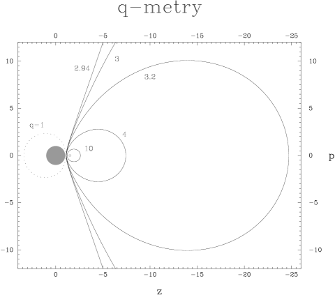
Figure 3: Sketch of the used coordinate system $(p,z)$ indicating the location of the early-type star (large gray circle) and the X-ray point source (tiny gray circle, not to scale) at a distance of 1.5 stellar radii, along with surfaces of constant $q$ (using a velocity law with $\gamma=1$ and $v_{0}=0.01$).

The X-ray point source at position ${\@vec{x}}_{\rm X}$ affects the normal abundance $q^{\prime}(x)$ of a certain ion in the wind. The degree at which the wind is disturbed is set by the parameter $q(\@vec{x})$ (Hatchett & McCray 1977):

$$q(\@vec{x})=\frac{v(x)}{v(x_{\rm X})}\frac{x^{2}}{(\@vec{x}-{\@vec{x}}_{\rm X})^{2}}\,.$$ (4)

Approximately, at all points on a surface of constant $q$, the X-rays remove the same fraction ${\eta}(q)$ of the ion under consideration (Tarter et al. 1969). This leaves only a $1-{\eta}(q)$ contribution of this ion to the source function $S(\@vec{x})$ and optical depth ${\tau}(\@vec{x})$. In our computations we adopt a region enclosed by a surface set by the value of $q$, with

$${\eta}(q(\@vec{x}))=\left\{\begin{array}[]{ll}\eta&\mbox{ for $q(\@vec{x})>q$ }\\ 0&\mbox{ else }\end{array}\right.$$ (5)

A negative value for $\eta$ enhances the abundance of the ion within the Strömgren zone. The X-ray point source is located inside a closed surface of constant $q$ if

$$q<q_{\rm critical}$$ (6)

with

$$q_{\rm critical}=\lim_{\begin{array}[]{l}x\rightarrow\infty\\ p=0\end{array}}q(\@vec{x})=\frac{1}{v(x_{\rm X})}\,.$$ (7)

Because of the singularity in ${\@vec{x}}_{\rm X}$ when calculating $q(\@vec{x})$, we excluded a small spherical region around the X-ray point source from the grid with a radius of one millionth of a stellar radius, which is of the order of the radius of a neutron star. As an example surfaces of constant q are shown (Fig. 3), for a velocity law with

$$\gamma=1\hskip 14.22636pt{\rm\&}\hskip 14.22636ptv_{0}=0.01$$ (8)

and putting the X-ray point source at

$$x_{\rm X}=1.5\,,$$ (9)

which corresponds to

$$v(x_{\rm X})=0.34\hskip 14.22636pt{\rm\&}\hskip 14.22636ptq_{\rm critical}=2.941\,.$$ (10)

The escape probability method (Castor 1970) makes a local approximation for the source function $S_{\nu}(x)$ at comoving frequency $\nu$, namely the Sobolev approximation

$$S_{\nu}(x)=\frac{{\beta}_{c}(x)I_{\nu}^{\ast}+\epsilon B_{\nu}(x)}{\beta+\epsilon}$$ (11)

Here, $\beta$ is the escape probability of a line photon; ${\beta}_{c}$ the penetration probability of a continuum photon; $\epsilon$ the ratio of collisional over radiative de-excitations; $B_{\nu}$ the Planck function at frequency $\nu$; and $I_{\nu}^{\ast}$ the stellar photospheric intensity at frequency $\nu$. Due to the relatively low density of in the stellar wind, the contribution of collisional (de)excitations to the source function of the UV resonance lines can be neglected:

$$\epsilon=0$$ (12)

The SEI method (Lamers et al. 1987) incorporates an exact integration of the radiative transfer equation, yielding the observed flux $F_{v}$ at the observed velocity $v$:

$$\frac{{\rm d}I_{\nu}}{{\rm d}{\tau}_{\nu}}=I_{\nu}-S_{\nu}\longmapsto F_{v}$$ (13)

The optical depth $\tau$ is parameterised as a function of velocity $v$:

$${\tau}(v)=\left\{\begin{array}[]{ll}T\frac{f(v)}{\int_{v_{0}}^{v_{1}}f(v){\rm d}v}&\mbox{ for $v\leq v_{1}$ }\\ 0&\mbox{ else }\end{array}\right.$$ (14)

with

$$f(v)=\left(\frac{v}{v_{1}}\right)^{{\alpha}_{1}}\left(1-\left(\frac{v}{v_{1}}\right)^{\frac{1}{\gamma}}\right)^{{\alpha}_{2}}\,.$$ (15)

The parameters $\alpha_{1}$ and $\alpha_{2}$ are defined as:

$${\alpha}_{1}=\frac{1}{\gamma}-t-2\hskip 14.22636pt{\rm\&}\hskip 14.22636pt{\alpha}_{2}=s\,,$$ (16)

where $t$ and $s$ parameterize the ionization fraction $\kappa_{\rm i}$ as a function of radial distance and velocity:

$$\kappa_{\rm i}(x)\propto x^{-s}v(x)^{-t}\,.$$ (17)

If $m$ is the dominant stage of ionization and $i$ is the ionization stage of the ion under consideration, then $t=m-i$. If the abundance of the dominant ion in the wind is constant, one gets

$${\alpha}_{1}=\frac{1}{\gamma}-2\hskip 14.22636pt{\rm\&}\hskip 14.22636pt{\alpha}_{2}=0\,.$$ (18)

If $v_{1}=1$, the ion is present up to the regions where the wind has reached its terminal velocity.

The intrinsic line profile resembles a Gaußian, with isotropic broadening ${\sigma}_{v}$ due to the thermal and turbulent motions — hereafter referred to as the “turbulence” (Lamers et al. 1987):

$${\Phi}({\Delta}v)=\frac{1}{\sqrt{\pi}{\sigma}_{v}}\exp{-\left(\frac{{\Delta}v}{{\sigma}_{v}}\right)^{2}}\,.$$ (19)

This introduces multiple resonance zones in the wind, which results in broader and stronger absorption effectively moving the emission peak towards longer wavelengths (in agreement with P-Cygni line obserservations).

In the case of doublets (most of the important UV resonance lines are doublets), depending on the doublet separation the source function of the red component includes a contribution from the blue component. Except for this coupling, the principle of the SEI code is the same as for singlets (Lamers et al. 1987). However, since we now include a Strömgren zone we can no longer use a one-dimensional radial grid to calculate the source function of the red component (as is the case for the SEI method). The contribution of the source function of the blue component to the source function of the red component depends on whether the coupled blue component points are situated inside the Strömgren zone. Hence the radial profile of the source function depends on the position of the Strömgren zone. This is solved by replacing the one-dimensional grid when calculating the source function of the red component by a two-dimensional axi-symmetric grid.

The SEI method allows the inclusion of a photospheric component in the input line spectrum, but we did not use this option in the model profiles shown below.

Figure 4: Changing the size of the X-ray ionization zone: SEI model profiles for a HMXB with a wind velocity law with $\gamma=1$, $v_{0}=0.01$ and ${\sigma}_{v}=0.2$, $x_{\rm X}=1.5$ ($v_{\rm X}=0.34$), doublet separation of $1.5$, integrated optical depth of the blue component of $T=100$ (twice that of the red component), dominant ionization stage in the uniformly ionized undisturbed wind, and no additional source of emission. The effect of different sizes $q$ of the Strömgren zone is illustrated (closed surfaces for $q>2.941$). The top panel shows the profile at X-ray eclipse (drawn line, $\phi=0$) and at $\phi=0.5$; the bottom panel presents the difference profile. Note that (much) less absorption is observed at $\phi=0.5$ when the X-ray source is in the line of sight.

Figure 5: The effect of turbulence: same as Fig. 4, but for $q=3.2$ and different levels of wind turbulence ${\sigma}_{v}$.

Figure 6: From weak to strong: same as Fig. 4, but for $q=3.2$ and illustrating the effect of increased integrated optical depth $T$.

Figure 7: Same as Fig. 4, but for $q=3.2$ and illustrating the effect of different parameterisations of the optical depth (via $\alpha_{1}$) and the velocity law (via $\gamma$).

Figure 8: Same as Fig. 4, but for $q=3.2$ and illustrating the effect of different distances $x_{\rm X}$ of the X-ray source.

The accuracy of the calculations depends on the grid $I_{\rm g}$, which samples the intrinsic line profile. The number of points used in the grid is $I_{\rm g,max}$. In the original code a choice of $I_{\rm g,max}=11$ yields satisfactory results, but if a Strömgren zone is included this value should be some two orders of magnitude larger to suppress the numerical noise. Stronger turbulence demands larger $I_{\rm g,max}$.

3.2 Application of the modified SEI model

To illustrate how the important model parameters affect the shape of the spectral line profile, model spectra are shown for a hypothetical resonance doublet of a HMXB system. The canonical model consists of a HMXB with $x_{\rm X}=1.5$, wind velocity law with $\gamma=1$, $v_{0}=0.01$ and ${\sigma}_{v}=0.2$, doublet separation of $1.5$, integrated optical depth of the blue component of $T=100$ (twice that of the red component), dominant ionization stage in the uniformly ionized undisturbed wind ($t,s=0$), no additional source of emission ($\epsilon=0$), no photospheric absorption profile, and a Strömgren zone of size $q=3.2$.

Figs. 4 to 8 illustrate the effect of varying several of these parameters. The top panels present the UV resonance profiles at two orbital phases: at X-ray eclipse ($\phi=0$, drawn line) a large fraction of the Strömgren zone is behind the OB supergiant so that only a small part of the observable stellar wind is affected. When the X-ray source is located in the absorbing column in front of the OB supergiant ($\phi=0.5$), the blue-shifted absorption trough is reduced in strength. Note that also the emission peak of the P-Cygni profile is affected, though less pronounced because the wind volume contributing to the P-Cygni emission is much larger in comparison to the volume of the absorbing column. The bottom panels show the difference spectra ($\phi=0.5$ minus $\phi=0$).

The size $q$ of the Strömgren zone strongly affects the spectral line variability (Fig. 4). Small Strömgren zones (large $q$) leave little trace in the spectral line profile, apart from some diminished absorption at $\phi=0.5$ at velocities between about $-v_{\rm X}$ and 0 (i.e. not centred at $-v_{\rm X}$). A larger Strömgren zone enhances the HM-effect especially near velocities $<-v_{\rm X}$, also reducing the absorption in the blue wing of the line profile, and reduces the emission at positive velocities at $\phi=0$ (notably in the red component of the doublet). Saturation is not maintained for Strömgren zones that cover a significant fraction of the hemisphere in front of the star. However, open Strömgren zones leave only a small area behind the primary unaffected (in the most extreme case this is a shadow wind), and hence cause diminished absorption and emission at all orbital phases, thereby reducing the contrast in line profile shape between transit and eclipse of the X-ray source. The appearance of the HM-effect is most prominent for $q{\sim}q_{\rm critical}$. The definition of $q$ allows a Strömgren zone extending into the X-ray shadow behind the supergiant; obviously, this can only happen if scattering of X-rays by ions in the stellar wind is important.

The presence of turbulence in the wind causes the line profile to broaden, which results in less pronounced emission (Fig. 5). The HM-effect is also smoothed in velocity space. The amplitude of variability at positive velocities and between 0 and $-v_{\infty}$ decreases, whilst the amplitude of variability in the blue wing ($v<-v_{\infty}$) increases. The blue wing variability becomes dominant in the case of strong turbulence. In the absence of turbulence it is difficult to hide the HM-effect unless the Strömgren zone is much smaller than the projected stellar disk.

Greater optical depth enhances the extent to which the absorption is maintained when the Strömgren zone moves through the line of sight (Fig. 6). Note that for heavily saturated lines with turbulence, as for unsaturated lines, it is not straightforward to determine the exact value of $v_{\infty}$, and careful modelling is required.

The ionization stage of the ion, relative to the dominant ionization stage in the (undisturbed) wind is of importance for the parameterisation and normalisation of the optical depth. If the ion corresponds to an ionization stage that is one level below the dominant ionization stage, then $\alpha_{1}=-2$ instead of $-1$ in the canonical example (see Eq. 16). For the same integrated optical depth, this would yield unsaturated and rather triangular shaped absorption profiles with little emission. In the opposite case, if the ion corresponds to one level above the dominant ionization stage, then $\alpha_{1}=0$. This yields a heavily saturated line profile with stronger emission and somewhat enhanced HM-effect in the absorption part between $-v_{\rm X}$ and $-v_{\infty}$, compared to the canonical case. From the normalisation of the optical depth (Eqs. 14 & 15) it follows that $\tau/T$ at $v=v_{\infty}$ ($=v_{1}$) is 0.010, 0.22, or 1.0 for $\alpha_{1}=-2$, $-1$ and 0, respectively. Scaling the total optical depth $T$ to 2200 and 22 for $\alpha_{1}=-2$ and 0, respectively, the line profiles and appearance of the HM-effect (Fig. 7) are similar to the canonical case. It may therefore be difficult to distinguish between different values of $\alpha_{1}$, and prior knowledge of the dominant ionization species is required.

The parameterisation of the optical depth involves the velocity law, and hence the parameter $\gamma$. Changing $\gamma$ from 1 to 0.5 requires rescaling to $q=1.87$, $\alpha_{1}=0$ and $T=22$ (Eqs. 4 & 15). The resulting variability is not exactly a scaled version of the canonical case (Fig. 7), because $q$ depends on both $v$ and $x$. Most notably, the blue wing HM-effect is stronger and saturation more difficult to maintain.

A different distance $x_{\rm X}$ of the X-ray source implies that different parts of the wind are probed. Changing to $x_{\rm X}=1.2$ and 2.0 requires rescaling to $q=6.2$ and 2.15, respectively. Increasing the distance of the X-ray source enhances the HM-effect in the blue wing at the expense of the HM-effect in the absorption part between $-v_{\rm X}$ and $-v_{\infty}$, and also makes it more difficult for a saturated line to remain saturated (Fig. 8). If the X-ray source is located close to the primary, then the HM-effect in the emission at positive velocities is less pronounced.

4 Model fits to the ultraviolet resonance lines of HD77581/Vela X-1 & HD153919/4U1700$-$37

Table 3: SEI model parameters for fits to the observed profiles and variability of UV resonance lines in the spectra of HD77581/Vela X-1 and HD153919/4U1700$-$37.

Line	$T$	$\alpha_{1}$	$\alpha_{2}$	$\sigma$	$v_{\infty}$	$q$
HD77581/Vela X-1:
N v	3	1	$-1$	0.45	600	2.9
Si iv	300	$-1$	0	0.45	600	2.9
C iv	200	0	0	0.45	600	2.9
Al iii	20	$-1$	0	0.45	600	2.9
HD153919/4U1700$-$37:
N v	30	0	0	0.15	1700	$>4$
Si iv	$2\times 10^{4}$	$-2$	0	0.15	1700	$>4$
C iv	5000	$-2$	0	0.15	1700	$>4$

The modified SEI code is used to fit the line profiles at two orbital phases ($\phi=0$, X-ray eclipse, and $\phi=0.5$) of N v, Si iv, C iv and Al iii resonance lines in HD77581/Vela X-1 and N v, Si iv and C iv in HD153919/4U1700$-$37. The models are constrained by the following conditions: (i) the values for $\gamma$, $v_{\infty}$, $\sigma$ and $q$ are the same for all lines in a given HMXB; (ii) the value for $x_{\rm X}$ follows from the orbital parameters (Table 1); (iii) the dominant ionization stage is estimated from the spectral type (Lamers et al. 1999). In HD77581 N²⁺, Si³⁺ and C²⁺ are expected to dominate, while in HD153919 probably N³⁺, Si⁴⁺ and C⁴⁺ dominate. Al²⁺ is assumed to dominate in HD77581, as the observed Al iii line is very strong. The ionization is uniform throughout the undisturbed wind, i.e. $\alpha_{2}=0$ (except N⁴⁺ in HD77581). Note that the N v line suffers from strong absorption by the wing of Ly-$\alpha$. A sudden jump in intensity near the maximum of the Si iv and C iv emission in HD153919/4U1700$-$37 is due to numerical difficulties. These lines were calculated by sampling the intrinsic line profile over $\pm 5\sigma$ with $I_{\rm g,max}=3333$ (instead of $\pm 3\sigma$ with $I_{\rm g,max}=1111$), suppressing the spikey feature by half. The resulting line profiles are shown in Figs. 9, 10 & 14 and the model parameters are listed in Table 3.

Figure 9: SEI models that approximately fit the observed line profiles and variability of Si iv, C iv and Al iii in the UV spectrum of HD77581/Vela X-1. Parameters are summarised in Table 3, and $v=1$ corresponds to 600 km s^-1.

Figure 10: Same as Fig. 9, but for the N v line in the UV spectrum of HD77581/Vela X-1 (see also Table 3).

The orbital modulation of the strong wind lines in HD77581 (with the exception of N v) is mainly due to the HM-effect. Some detailed changes are probably related to the accretion flow in the system (Sadakane et al. 1985; Kaper et al. 1994); since these structures are not included in the model, they cannot be reproduced. The modified SEI model can naturally explain the (near) absence of orbital modulation in the resonance lines of HD153919, which is one of the main motivations for this study.

4.1 HD77581/Vela X-1

4.1.1 Strong wind lines

Adopting the ionization structure of the stellar wind as expected for single stars of the same effective temperature as HD77581, and adopting $v_{\infty}=600$ km s^-1, the shape and variability of the Si iv, C iv and Al iii (²S-²P⁰ resonance doublet: restwavelengths 1854.716 & 1862.790, separation 1302 km s^-1) line profiles are reproduced rather well (Fig. 9, compare with Fig. 11).

                 

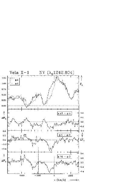
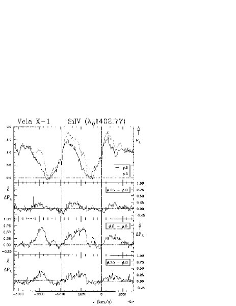
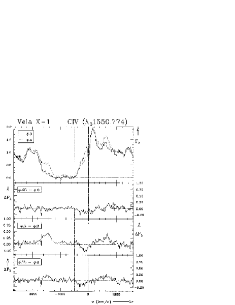
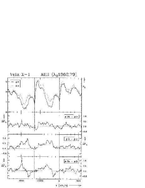
Figure 11: Phase $\phi=0$ (solid) and $\phi=0.5$ (dotted) spectra for the N v, Si iv, C iv and Al iii resonance lines in HD77581/Vela X-1, with rest wavelengths indicated by vertical dashed lines and the velocity axis defined by the redmost component (labelled above the graph). The differences between the $\phi=0.25$, 0.5 and 0.75 spectra relative to the $\phi=0$ spectrum are plotted below.

       

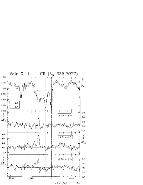
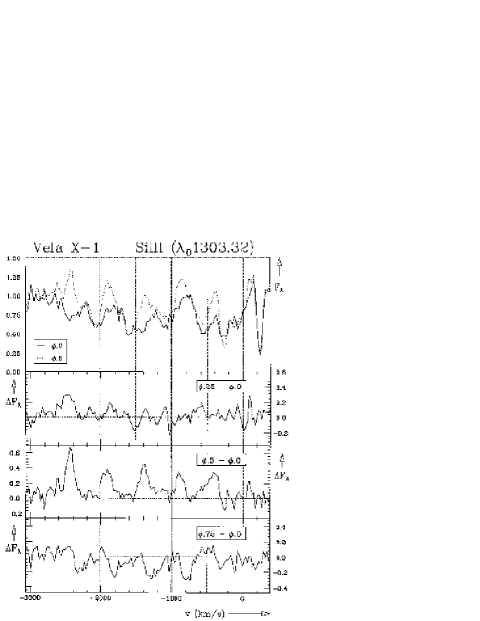
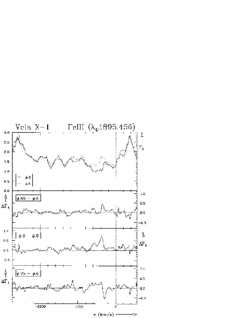
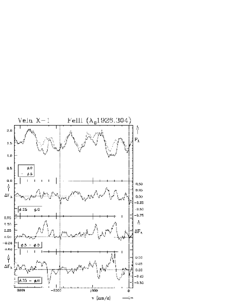
Figure 12: Same as Fig. 11, but for C ii, Si iii and Fe iii.

The N v line profile (Fig. 10, calculated with $I_{\rm g,max}=5555$), however, cannot be modelled using a normal ionization balance that would yield an extremely profound HM-effect, especially at the inner part of the absorption (Fig. 10a), which is not observed (Fig. 11). Instead, the observations seem to favour the degree of ionization to increase with distance to the primary: $\alpha_{2}=-1$ gives an acceptable fit, suppressing the orbital modulation of the absorption trough, while preserving some of the emission (Fig. 10b). The line profile and its modulation are very similar for $\alpha_{1}=0$ or $-1$ (Fig. 10c), only requiring a slightly larger integrated optical depth ($T$). If $\alpha_{1}{\vbox{\hbox{$<$}\offinterlineskip\hbox{$\sim$}}}-2$, however, much of the absorption arises from material at extreme velocities, causing the absorption profile to extend up to large positive velocities beyond the severely diminished emission. The absorption observed longward of the N v line can be attributed to a C iii line.

The slope of the blue absorption wing (especially in Si iv and C iv, see Fig. 2) indicates that the level of saturation (deeper and at velocities slightly more negative than $-v_{\infty}$) is not reproduced well by the SEI turbulence recipe (Eq. 19). The shocked wind structure produced by numerical simulations (Owocki 1994), however, seem to predict more material at extreme velocities (rather than gaußian turbulence). Furthermore, the turbulence may not be uniform throughout the wind, as it is assumed here.

4.1.2 Variations in addition to the HM-effect: evidence for a photo-ionization wake

The main discrepancy between the model and observations of HD77581/Vela X-1 is the $-400$ to 0 km s^-1 region, where the observed intensity is often lower at $\phi=0.5$ than at $\phi=0$, contrary to what the HM-effect predicts. This may be due to the presence of a photo-ionization wake that enhances absorption at phases $\phi{\vbox{\hbox{$>$}\offinterlineskip\hbox{$\sim$}}}0.5$ (Kaper et al. 1994). The photo-ionization wake, as observed in strong optical lines like the hydrogen Balmer lines and He i lines in the spectrum of HD77581, is situated close to the star at the trailing border of the ionization zone.

This effect is especially pronounced in N v (Fig. 11), possibly as a result of a change in ionization degree within the photo-ionization wake. Enhanced absorption is seen between $+200$ and $-600$ km s^-1 ($=-v_{\infty}$), with its maximum evolving towards more negative velocities from $\phi=0.25$ to $\phi=0.75$. Absorption at $\phi=0.25$ (or enhanced emission at $\phi=0$) extends up to $+600$ km s^-1.

Similar enhanced absorption is seen in Si iv, C iv and Al iii (Fig. 11) at $-200$ and $-300$ to $-400$ km s^-1 around $\phi=0.5$ and 0.75, respectively, and perhaps already around $\phi=0.25$. The enhanced absorption due to the photo-ionization wake may have reduced the amplitude of the HM-effect seen between $-600$ and $-400$ km s^-1.

Several weaker UV lines also show orbital modulation. The ²P⁰-²D resonance doublet of C ii at 1334.5323 and 1335.7077 Å (Fig. 12) is sufficiently strong to show the HM-effect between 0 and about $+700$ km s^-1 and between about $-400$ and $-600$ km s^-1, but slightly enhanced absorption at $-300$ km s^-1 around $\phi=0.75$ may be attributed to the photo-ionization wake.

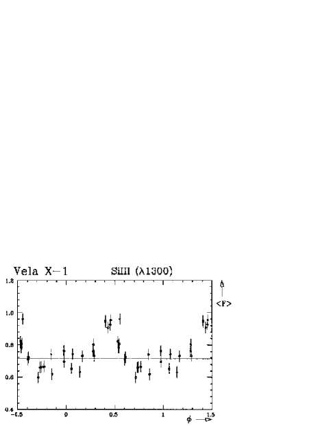
Figure 13: Lightcurve for the integrated flux in the Si iii resonance lines around 1300 Å in HD77581/Vela X-1. The dotted line indicates the flux level around $\phi=0$.

The strongly variable ³P⁰-³P multiplet UV 4 of Si iii (Fig. 12) consists of 6 components, of which 2 are blended: the pattern of variability is repeated five-fold. The absorption is diminished at $-400$ km s^-1 at $\phi=0.5$ due to the HM-effect, but enhanced at $-300$ km s^-1 at $\phi=0.75$ due to the photo-ionization wake. In Fig. 13 a lightcurve is plotted for the spectral region between 1292 and 1303 Å — corresponding to $-2600$ and $-70$ km s^-1, respectively. Absorption is minimal between $\phi=0.4$ and 0.5, and strongest between $\phi=0.7$ and 0.8. The blending of the Si iii components makes it difficult to detect variability at $-600$ km s^-1, although there is a hint for diminished absorption at $\phi=0.5$ at this velocity in the bluemost component at 1294.543 Å. The ¹S-¹P⁰ (multiplet UV 2) resonance singlet of Si iii at 1206.51 Å could not be studied, due to the severe interstellar extinction and the strong Ly$\alpha$ geocoronal line at 1215.34 Å in the neighbouring echelle order. The subordinate singlets of ¹P⁰-¹S multiplets UV 9 and UV 10 of Si iii at 1417.24 and 1312.59 Å, respectively, do not show variability, although the lines are clearly present in the spectrum — particularly the UV 9 singlet. The ²P⁰-²S resonance doublet of Si ii at 1304.372 Å ($+240$ km s^-1 in Fig. 12) does not show any variability either, as it is of interstellar origin.

The spectral region around 1900 Å is dominated by numerous lines of Fe iii, of which the a⁷S-z⁷P⁰ multiplet 34 is the strongest. It consists of 3 widely separated components at 1895.456, 1914.056 and 1926.304 Å (Fig. 12). They all clearly show the diminished absorption at $-400$ and $-600$ km s^-1 around $\phi=0.5$ due to the HM-effect, and enhanced absorption at $-300$ km s^-1 around $\phi=0.75$ due to the photo-ionization wake, exactly as observed in the Al iii resonance doublet. Some confusion arises from the presence of 2 lines of the a⁵G-z⁵H⁰ multiplet 51 of Fe iii at 1922.789 and 1915.083 Å, corresponding to $-550$ and $-1750$ km s^-1 with respect to 1926.304 Å, respectively. Multiplet 51 shows the same behaviour of the absorption near $-300$ and $-400$ km s^-1 as multiplet 34, but not the $-600$ km s^-1 absorption.

Figure 14: SEI models that approximately fit the observed line profiles and variability of N v, Si iv and C iv in the UV spectrum of HD153919/4U1700$-$37. Parameters are summarised in Table 3, and $v=1$ corresponds to 1700 km s^-1.

In conclusion, the orbital modulation of both the strong wind lines and other lines in the UV spectrum of HD77581 indicates the presence of two absorption components that are not included in the SEI modelling. The most prominent of these can be explained by a photo-ionization wake, causing additional absorption in the line-of-sight at $v\sim-200$ km s^-1 around $\phi=0.5$ and at $v\sim-300$ km s^-1 around $\phi=0.75$. In addition, at $v\sim-600$ km s^-1, i.e. the terminal velocity of the wind of HD77581, more absorption is present outside the Strömgren zone than the SEI model reproduces. This might reflect the stellar wind structure at larger distances from the star: the velocity may be lower and the density higher after the wind has passed through the Strömgren zone compared to an undisturbed wind.

4.2 HD153919/4U1700$-$37

The shape and (lack of) orbital modulation of the line profiles in HD153919/4U1700$-$37 are reproduced well (Fig. 14). The exact value for $q$ is hard to determine because of the (near) absence of the HM-effect due to a combination of strong absorption and the presence of turbulence, yet it is clear that $q<4$ would definitely yield a too strong HM-effect. Also, the HM-effect is predicted to appear strongest at velocities between $-v_{\infty}$ and 0, implying that any variations in the blue absorption wing (at $|v|>v_{\infty}$) without accompanying HM-effect at smaller velocities must be due to some other mechanism, e.g. Raman-scattered far-UV emission lines (Kaper et al. 1990).

5 Discussion

The adapted SEI model reproduces the HM-effect in HD77581/Vela X-1, and naturally explains the lack of any (clear) HM-effect observed in the dense wind system HD153919/4U1700$-$37. Absorption components that are seen both in the strong wind lines and additional weaker lines in the UV spectrum of HD77581/Vela X-1 and that could not be reproduced by the adapted SEI model can be explained by a photo-ionization wake. The orbital modulation of the resonance lines in the UV spectra of the five HMXBs studied here shows a clear trend of the size of the Strömgren zone to increase with higher X-ray luminosity.

5.1 Terminal velocities and turbulence

The terminal velocity $v_{\infty}$ may be estimated from a comparison of an appropriate model line profile with the observed line profile. It is best derived from moderately saturated profiles, in which case the maximum absorption in the $\phi=0.5$ line profile occurs at the terminal velocity.

The terminal velocity for HD77581/Vela X-1 is thus estimated to be $v_{\infty}=600$ km s^-1, much slower than previously reported (1105 km s^-1 Prinja et al. 1990). For HD153919/4U1700$-$37 we estimate $v_{\infty}=1700$ km s^-1 (Prinja et al. 1990: 1820 km s^-1). These values should be correct to within $100$ km s^-1. The low resolution IUE spectra show that the wind in HDE226868/Cyg X-1 is faster (marginally resolved: $1000<v_{\infty}<1500$ km s^-1) than in Sk-Ph/LMC X-4 and Sk 160/SMC X-1 (unresolved: ${\vbox{\hbox{$<$}\offinterlineskip\hbox{$\sim$}}}600$ km s^-1, see also Hammerschlag-Hensberge et al. 1984 for Sk 160/SMC X-1). HST/STIS spectra of the N v, Si iv and C iv lines in Sk-Ph/LMC X-4 around $\phi=0$ suggest a terminal velocity of $\sim 500$ km s^-1, even though wind velocities up to $\sim 1200$ km s^-1 occur (Kaper et al. in preparation).

Single (galactic) O-type and early-B-type stars are known to have a fairly constant ratio of terminal over escape velocity $v_{\infty}/v_{\rm esc}\sim 2.5$, where

$$v_{\rm esc}=\sqrt{\frac{2GM(1-\Gamma)}{R}}$$ (20)

with

$$\Gamma=2.658\times 10^{-5}\frac{L}{L_{\odot}}\left(\frac{M}{M_{\odot}}\right)^{-1}$$ (21)

for a typical Population I star (e.g. Groenewegen et al. 1989). This is also true at temperatures between $\sim 1.1$ and $2.1\times 10^{4}$ K but then $v_{\infty}/v_{\rm esc}\sim 1.3$ (Lamers et al. 1995). The terminal velocities for the primary stars of the five HMXBs studied here are, with the possible exception of HDE226868, low compared to single stars of the same effective temperature (Table 4 & Fig. 15). Especially the two magellanic stars have very low terminal velocities, which may at least partly be due to their subsolar metallicity and hence lower radiation-force multiplier (Garmany & Conti 1985; Prinja 1987; Kudritzki et al. 1987) — which is also found for dust-driven winds of Asymptotic Giant Branch stars (e.g. van Loon 2000).

The Strömgren zone could inhibit acceleration of the stellar wind material flowing through it, not only resulting in an ionization wake but possibly also leading to a slower terminal velocity of the wind. This scenario only works if the Strömgren zone is sufficiently large and the orbital period sufficiently short that all wind material leaving the star passes through the Strömgren zone before having reached the terminal velocity. The magellanic systems indeed must have very extended Strömgren zones leaving only a small region at the opposite side of the primary unaffected by the X-ray source (i.e. a shadow wind), and their orbital periods are rather short. However, the Strömgren zones in HD77581/Vela X-1 and HD153919/4U1700$-$37 are closed surfaces, and certainly do not occupy more than half of the circumstellar space. Within half their orbital periods of 4.5 and 1.7 days, respectively, their stellar winds ought to already have accelerated to velocities approaching the terminal velocity as if it were from a single star.

A viable alternative is that the $\Gamma$ factors for single stars are not applicable to stars in interacting binaries. HMXBs primaries may have already lost a significant fraction of their initial mantle mass, causing them to be undermassive for their luminosity (Conti 1978; Kaper 2001). This seems to be confirmed when comparing the primary star masses (Table 1) with Table 3 in Howarth & Prinja (1989). Hence we may have under-estimated $\Gamma$ and over-estimated $v_{\rm esc}$.

Table 4: Ratios of terminal velocity $v_{\infty}$ and escape velocity $v_{\rm esc}$, and turbulent velocities $\sigma_{v}$ of the primary stars in the HMXBs, together with their effective temperatures $T_{\rm eff}$ and $\Gamma$ values estimated from Lamers et al. (1995).

Primary	$T_{\rm eff}$ (K)	$\Gamma$	$v_{\infty}/v_{\rm esc}$	$\sigma_{v}$
HDE226868	30500	0.34	1.8—2.8
Sk-Ph	36000	0.16	$<$ $\sim$ 0.8
Sk 160	26000	0.18	$<$ $\sim$ 1.1
HD77581	23400	0.18	1.3	0.45
HD153919	37200	0.34	2.0	0.15

Figure 15: Ratio of terminal over escape velocity for the primary stars in the HMXBs studied here (solid dots), compared to single stars (circles) from Lamers et al. (1995). HMXB members have low terminal velocities for their effective temperatures.

A turbulence description has been employed to account for material at velocities deviating from the bulk flow that obeys a velocity law according to standard radiation-driven wind theory. The $\sigma$ is the typical deviation in units of $v_{\infty}$. To approximately describe both the undisturbed wind and X-ray ionized components in the line profiles of HD77581/Vela X-1 a very large value for $\sigma$ needs to be invoked ($\sigma_{v}\sim 0.45$), whereas for HD153919/4U1700$-$37 a much smaller value suffices ($\sigma_{v}\sim 0.15$). In absolute terms the turbulence in these two HMXBs is very similar, though: $v_{\rm turb}=270$ and 255 km s^-1, respectively. These values are typical for winds from O-type stars for which $v_{\rm turb}$ has been found to be largely independent of $T_{\rm eff}$ (Groenewegen et al. 1989). As mentioned before, we find indications for the deviations from the monotonic velocity law to resemble a shocked wind structure rather than uniform turbulence.

5.2 Ionization fractions in the stellar wind

Table 5: Ionization fractions $\kappa_{\rm i}$ for several ions in the stellar winds of HD77581/Vela X-1 and HD153919/4U1700$-$37 as derived from SEI model parameters, adopting mass-loss rates $\dot{M}$ from H$\alpha$ line profile modelling (Schröder et al. in preparation) and using solar element abundances $A$. Ionization fractions from work on single stars (Lamers et al. 1999) are given for comparison.

Line	$\lambda_{0}$ (Å)	$f_{\rm line}$	$T$	$A$	$\dot{M}_{{\rm H}\alpha}$ (M⊙ yr-1)	$\kappa_{\rm i}$	$\kappa_{\rm i,Lamers}$
HD77581/Vela X-1:
N v	1238.821	0.152	3	$1.1\times 10^{-4}$	$1\times 10^{-6}$	$5\times 10^{-4}$	$3\times 10^{-5}$
Si iv	1393.755	0.528	300	$3.5\times 10^{-5}$	$1\times 10^{-6}$	$4\times 10^{-2}$	$1\times 10^{-2}$
C iv	1548.20	0.194	200	$3.6\times 10^{-4}$	$1\times 10^{-6}$	$6\times 10^{-3}$	$1\times 10^{-2}$
Al iii	1854.716	0.560	20	$3.0\times 10^{-6}$	$1\times 10^{-6}$	0.3	$<1$
HD153919/4U1700$-$37:
N v	1238.821	0.152	30	$1.1\times 10^{-4}$	$1\times 10^{-5}$	$2\times 10^{-3}$	$3\times 10^{-3}$
Si iv	1393.755	0.528	$2\times 10^{4}$	$3.5\times 10^{-5}$	$1\times 10^{-5}$	$\sim 1$	$1\times 10^{-3}$
C iv	1548.20	0.194	5000	$3.6\times 10^{-4}$	$1\times 10^{-5}$	$6\times 10^{-2}$	$3\times 10^{-3}$

In principle, the mass-loss rate may be estimated from the integrated optical depth $T$ of a resonance line:

$$T=\frac{\pi e^{2}}{m_{e}c}f_{\rm line}\lambda_{0}N_{\rm i}v_{\infty}^{-1}$$ (22)

with $f_{\rm line}$ the oscillator strength of the transition in terms of the harmonic oscillator $\pi e^{2}/m_{e}c$, $\lambda_{0}$ the rest wavelength of the transition, and $N_{\rm i}$ the column density of the ion:

$$N_{\rm i}=\int_{R_{\star}}^{\infty}n_{\rm i}(r){\rm d}r$$ (23)

with $n_{\rm i}$ the number density of the ion. The continuity equation yields

$$\dot{M}=4\pi r^{2}v(r)\left<m\right>\frac{n_{\rm i}(r)}{A_{\rm i}}$$ (24)

with $\rho$ the mass density, $\left<m\right>$ the mean mass of an ion in the wind, and $A_{\rm i}$ the ion abundance by number. The mass-loss rate $\dot{M}$ can now be estimated from observed quantities in the following way:

$$\dot{M}=\frac{4m_{e}c}{e^{2}f_{\rm line}\lambda_{0}}\left<m\right>R_{\star}v_{\infty}^{2}\psi\frac{T}{A_{\rm i}}$$ (25)

with

$$\psi=\left\{\begin{array}[]{lll}(1-\gamma)&\mbox{\hskip 8.53581pt for \hskip 2.84526pt $0{\leq}\gamma<1$}&\mbox{\hskip 2.84526pt \& \hskip 2.84526pt $v_{0}=0$}\\ (v_{0}-1)/\ln{v_{0}}&\mbox{\hskip 8.53581pt for \hskip 15.649pt $\gamma=1$}&\mbox{\hskip 2.84526pt \& \hskip 2.84526pt $v_{0}>0$}\end{array}\right.$$ (26)

For our choice of $\gamma=1$ & $v_{0}=0.01$ the numerical factor $\psi=0.215$. Adopting a mean nucleus mass $\left<m\right>=2.2624\times 10^{-24}$ g (Lamers et al. 1999) the product of mass-loss rate $\dot{M}$ and ion abundance $A_{\rm i}$ can be calculated for the resonance lines in HD77581/Vela X-1 and HD153919/4U1700$-$37.

In practice, however, the limited knowledge of the ionization balance in the winds of OB supergiants makes the derived mass-loss rates highly unreliable. Instead, the ionization fractions of the ions may be derived when other, more reliable estimates for the mass-loss rate are available. For resonance lines the excitation fraction of the ion that produces the line is unity, and the ion abundance $A_{\rm i}$ is the product of the ionization fraction $\kappa_{\rm i}$ and elemental abundance $A$ (by number). Assuming solar abundances (Anders & Grevesse 1989), the ionization fraction may be derived using Eq. 25.

Lamers et al. (1999) found $\kappa_{\rm i}$ to depend on both radiation temperature and density, with the radiation temperature scaling approximately linearly with $T_{\rm eff}$. The empirical dependencies of $\kappa_{\rm i}$ on density were contrary to the expected ionization balance, however, and it was argued that the empirical relations may suffer from selection effects. Therefore, we only consider their empirical relations between $\kappa_{\rm i}$ and $T_{\rm eff}$.

Schröder et al. (in preparation) model the H$\alpha$ profiles of OB supergiants in HMXBs. They derive mass-loss rates for HD77581 ($\dot{M}\sim 1.0\times 10^{-6}$ M_⊙ yr^-1) and HD153919 ($\dot{M}\sim 1.0\times 10^{-5}$ M_⊙ yr^-1), which are comparable to those derived for single stars of similar spectral type (Howarth & Prinja 1989). Combining their results with the results from the SEI models, ionization fractions $\kappa_{\rm i}$ are estimated for the N⁴⁺, Si³⁺ and C³⁺ (and Al²⁺) ions in the (undisturbed) stellar winds of HD77581 and HD153919 (Table 5). These are then compared with the ionization fractions estimated from Fig. 3 in Lamers et al. (1999), taking into account their lower and upper limits.

The ion fractions derived from the SEI modelling for HD77581/Vela X-1 are in agreement with the predictions for single stars by Lamers et al. (1999), except for the N⁴⁺ abundance which is observed to be an order of magnitude higher than predicted. This may be due to either super-ionization or nitrogen over-abundance (or both). Auger ionization (Cassinelli & Olson 1979) is sometimes invoked to explain strong N v resonance lines. Unless the density becomes very high, Auger ionization increases with the velocity in the wind, and may originate in the high-velocity extrema of a shocked wind. This might mimic a moderate increase of ionization fraction with distance, as required to reproduce the observed line profile and variability of the N v line in HD77581/Vela X-1. On the other hand, nitrogen over-abundance at the surface of HD77581 may have resulted from (i) the transfer in the past of nitrogen-enriched material from the progenitor of Vela X-1 onto HD77581, or (ii) strong mass loss exposing deeper layers mixed with the products of nuclear burning. Kaper et al. (1993) note that HD77581 might be a BN star.

For HD153919/4U1700$-$37 the opposite is found: the observed ionization fraction of N⁴⁺ agrees very well with the predictions, whereas the ionization fractions of Si³⁺ and C³⁺ are observed to be (much) higher than predicted. Perhaps these are the dominant ionization states for silicon and nitrogen in the stellar wind of HD153919, rather than Si⁴⁺ and C⁴⁺. Still, an ionization fraction $\kappa_{\rm i}\sim 1$ for Si³⁺ is unrealistic for a multi-level atom, and hence the SEI model must have over-estimated the integrated optical depth of the Si iv line in HD153919/4U1700$-$37. If indeed the degree of ionization in the wind of HD153919 is lower than that predicted for single stars, this would mean that — like in the wind of HD77581 — N⁴⁺ is in fact overabundant in the wind of HD153919.

5.3 Size of the Strömgren zone

The size of the Strömgren zone, indicated by a particular value of the parameter $q$, is related to the ionization parameter $\xi$ as

$$\xi=\frac{qL_{\rm X}}{n_{\rm X}a^{2}}$$ (27)

where $a$ is the distance between the centres of the primary and the X-ray source. The ionization parameter can be interpreted as a measure for the number of X-ray photons per particle. The ionization balance in the stellar wind is mostly affected by soft X-ray photons. In common with previous models of the X-ray ionization of stellar winds in HMXBs, we assume the dominant source of opacity for soft X-rays is oxygen (Hatchett & McCray 1977). Masai (1984) has objected that this assumption may not be valid if He iiis present, but incorporating the effects of a He ii/He iii ionization front would be beyond the scope of this paper. As a consequence of our assumption, the sharp boundaries between the X-ray ionized and the undisturbed stellar wind coincide for ions like C³⁺, Si³⁺ and N⁴⁺ (cf. Kallman & McCray 1982; McCray et al. 1984). Hence the edge of the Strömgren zone is given by a particular value for $\xi$ that corresponds to the boundary at which oxygen is being completely ionized by the X-ray source, and depends on the shape of the X-ray spectrum and the oxygen abundance (Hatchett et al. 1976).

Accretion of matter onto a star moving through a medium was first described by Bondi & Hoyle (1944). Their concept was applied to HMXBs by Davidson & Ostriker (1973). In an HMXB the compact object has a velocity $v_{\rm rel}$ relative to the stellar wind flow:

$$v_{\rm rel}^{2}=v_{\rm wind}^{2}+(|v_{\rm X}-v_{\star}|-\frac{R_{\star}}{a}v_{\rm rot})^{2}$$ (28)

with stellar wind velocity $v_{\rm wind}$ near the X-ray source (which may be lower than implied by the undisturbed wind velocity law; see Section 5.1), orbital velocity $v_{\rm X}$ of the X-ray source, and orbital velocity $v_{\star}$, stellar radius $R_{\star}$ and rotation velocity $v_{\rm rot}$ of the primary. Kaper (1998) finds that generally $v_{\rm rel}\sim\frac{1}{2}v_{\rm wind}$. Stellar wind matter is accreted onto the compact object if it approaches within an accretion radius approximately given by

$$r_{\rm acc}=\frac{2GM_{\rm X}}{v_{\rm rel}^{2}}$$ (29)

with $M_{\rm X}$ the mass of the compact object. The X-ray luminosity due to the release of gravitation energy of the matter being accreted onto the surface of the compact object with radius $R_{\rm X}$ is

$$L_{\rm X}=\pi\zeta r_{\rm acc}^{2}v_{\rm rel}\rho_{\rm X}\frac{GM_{\rm X}}{R_{\rm X}}$$ (30)

where $\rho_{\rm X}$ is the mass density of the stellar wind near the compact object, and $\zeta$ is an efficiency parameter ($\zeta\sim 0.1$ for accretion onto a neutron star). Hence we obtain

$$q=\frac{\xi R_{\rm X}a^{2}}{4\pi\zeta\left<m\right>}\left(\frac{v_{\rm rel}}{GM_{\rm X}}\right)^{3}$$ (31)

The size of the Strömgren zone depends on: (1) the dimensions of the compact object via $R_{\rm X}$, $M_{\rm X}$ and $\xi$ (by the shape of the X-ray spectrum); (2) the orbit via $a$ and $v_{\rm rel}$ (by the orbital velocity); (3) the wind flow via $v_{\rm rel}$; (4) and the abundances in the wind via $\left<m\right>$ and $\xi$ (by the oxygen abundance). The size of the Strömgren zone does not, however, explicitly depend on the mass-loss rate nor on the X-ray luminosity.

Table 6: Critical, expected and observed sizes of the Strömgren zones in the five HMXBs (the smaller $q$, the larger the Strömgren zone).

HMXB	$q_{\rm critical}$	$q_{\rm expected}$	$q_{\rm observed}$
HDE226868/Cyg X-1	1.7	1.7—5.0	${\vbox{\hbox{$<$}\offinterlineskip\hbox{$\sim$}}}1.7$
Sk-Ph/LMC X-4	2.7	$<$1.6—4.5	$<2.7$
Sk 160/SMC X-1	2.9	$<$6.3—17	${\ll}2.9$
HD77581/Vela X-1	2.7	10—24	$2.9$
HD153919/4U1700$-$37	2.0	177—215	$>4.0$

From the time sequence of the integrated line variability (Figs. 1 & 2) and the modelling of the line profile variability it is already clear that the Strömgren zone is largest for Sk-Ph/LMC X-4 and especially Sk 160/SMC X-1: their zones must extend far beyond the primary as seen from the X-ray source, and the stellar wind is undisturbed only in a small shadow region behind the primary. The Strömgren zone is smaller but still very extended for HDE226868/Cyg X-1 where the variability due to the HM-effect is continuous over the orbit. HD77581/Vela X-1 has an again smaller and now closed Strömgren zone, but it still occupies a considerable fraction of the wind volume. The (by far) smallest Strömgren zone is found for HD153919/4U1700$-$37.

The critical and expected sizes of the Strömgren zones for the five HMXBs are listed in Table 6. The $q_{\rm critical}$ is calculated assuming a velocity law according to Eq. (2) with $v_{0}=0.01$ and $\gamma=1$. The $q_{\rm expected}$ is calculated assuming $\xi=10^{3}$ (Hatchett & McCray 1977) for a typical X-ray spectrum, $\zeta=0.1$, and $R_{\rm X}=10$ km for $M_{\rm X}=1.4$ M_⊙ and $R_{\rm X}{\propto}M_{\rm X}$. The range in values results from either assuming co-rotation of the primary with the orbit or no rotation of the primary (and the uncertainty about $v_{\infty}$ for Cyg X-1, LMC X-4 and SMC X-1). The observed sizes of the Strömgren zone are in reasonable agreement with the expected sizes that, in general, seem to have been somewhat under-estimated. This could easily be solved if for instance the accretion efficiency $\zeta$ were twice as large. In particular, $\zeta$ increases with larger mass and smaller radius of the compact object (Shakura & Sunyaev 1973), which would yield an accretion efficiency for the black-hole candidate Cyg X-1 significantly larger than 10%.

6 Summary

An analysis is presented of a large set of IUE spectra for five HMXBs: HDE226868/Cyg X-1, Sk-Ph/LMC X-4, Sk 160/SMC X-1, HD77581/Vela X-1 and HD153919/4U1700$-$37. We compared their spectra and variability, and adapted the SEI radiation transfer code for modelling the variability of resonance lines in HMXBs. From model fits for HD77581/Vela X-1 and HD153919/4U1700$-$37 we derive terminal velocities and ionization fractions of their stellar winds, as well as the sizes of the Strömgren zone created in the wind by the X-ray source. For three other HMXBs (HDE226868/Cyg X-1, Sk-Ph/LMC X-4 and Sk 160/SMC X-1) only rough estimates are derived for the terminal velocity and size of the Strömgren zone.

The adapted SEI model reproduces the Si iv, C iv and Al iii resonance line profiles and their orbital modulation in HD77581/Vela X-1, with additional absorption components attributed to a photo-ionization wake. The N v resonance line in HD77581/Vela X-1 is more difficult to model, and it seems to be severely affected by the photo-ionization wake. The N v, Si iv and C iv line profiles in HD153919/4U1700$-$37 are well reproduced by the adapted SEI model; their lack of orbital modulation is due to the dense stellar wind and low X-ray luminosity.

OB supergiants in HMXBs have lower terminal velocities than single stars of similar spectral type, possibly due to a lower effective gravity of the Roche-Lobe filling primary. Ionization fractions in the stellar wind of HD77581/Vela X-1 agree with predictions for single stars, except for an overabundance of N⁴⁺ ions in the wind of HD77581. This may be due to super-ionization possibly resulting from X-ray emission from shocks at the base of the wind, or nitrogen overabundance due to mass-transfer from the progenitor of Vela X-1 or extensive mass loss from HD77581 itself. The N⁴⁺ abundance in the stellar wind of HD153919/4U1700$-$37 agrees very well with predictions for single. However, the ionization fractions of the other ions (Si³⁺ and C³⁺) are much lower than predicted, suggesting a generally lower ionization of the stellar wind of HD153919 than what is predicted for single stars. This would then infer an N⁴⁺ over-abundance in the stellar wind of HD153919. The sizes of the Strömgren zones are in fair agreement with the expectations from standard Bondi & Hoyle accretion, and they are larger for more luminous X-ray sources.

Appendix A X-ray eclipse spectra

Averages of spectra near $\phi=0$ (eclipse of the X-ray source) are a fair representation of the “undisturbed” stellar wind. The low-resolution spectra of HDE226868/Cyg X-1, Sk 160/SMC X-1, and Sk-Ph/LMC X-4 all contain the strong geocoronal Lyman-$\alpha$ emission line at 1215.34 Å, and the resonance lines of C iv near 1550 Å and Si iv near 1400 Å (Fig. 1). These are much stronger in HDE226868/Cyg X-1 than in the two Magellanic Cloud members that both have a lower metalicity than their counterparts in the Milky Way.

Also immediately clear is the difference between the continua of HDE226868/Cyg X-1 and the two Magellanic Cloud members. Due to the high extinction towards HDE226868/Cyg X-1, its continuum is tilted both at the 1200 Å side (dust and hydrogen) and at the 2100 Å side (grains or large molecules). The Magellanic Cloud members are much less affected by interstellar extinction.

Figure 16: X-ray eclipse spectra of HDE226868/Cyg X-1, Sk 160/SMC X-1, and Sk-Ph/LMC X-4.

The high resolution spectra have not been flux calibrated in an absolute sense, therefore the shape of the continuum in Figs. A2 and A3 does not represent the shape of the continuum as it entered the telescope.

The geocoronal Ly-$\alpha$ line and the resonance lines of N v, Si iv, C iv and Al iii are the most prominent features in the spectrum of HD77581/Vela X-1 (Fig. A2, top). N v and Al iii are very strong for its spectral type. Notice the rich Fe iii spectrum at wavelengths longer than $\sim 1880$ Å, the Fe iv spectrum between $\sim 1480$ Å and 1880 Å, and the lack of Fe v and Fe vi at wavelengths $\vbox{\hbox{$<$}\offinterlineskip\hbox{$\sim$}}1480$ Å.

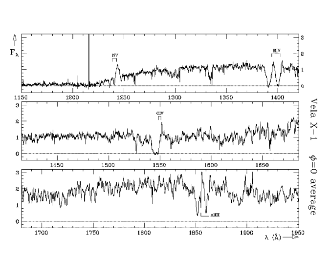
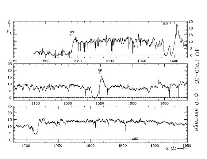
Figure 17: X-ray eclipse spectra of HD77581/Vela X-1 (top) and HD153919/4U1700$-$37 (bottom).

In the spectrum of HD153919/4U1700$-$37 (Fig. A2, bottom) the resonance lines of N v, Si iv and C iv and the subordinate line of N iv at 1718.551 Å are very strong. The resonance line of Al iii is mainly interstellar. Notice that the Fe iii and Fe iv spectra are absent, whilst at wavelengths $\vbox{\hbox{$<$}\offinterlineskip\hbox{$\sim$}}1480$ Å the spectrum is crowded with lines of Fe v and Fe vi. This contrast with HD77581/Vela X-1 is due to the higher photospheric temperature of the O6.5 Iaf⁺ star HD153919 compared to the B0.5 Iab star HD77581. The stronger P-Cygni lines of Si iv and C iv in HD153919/4U1700$-$37 reflect the denser and faster stellar wind of HD153919 compared to HD77581. Note that the N v emission is stronger in HD77581/Vela X-1.

Appendix B Normalisation and continuum variability

Comparison of column densities towards the primary as derived from line absorption requires the continuum to be normalised to eliminate continuum variability of the primary — which is mainly due to tidal deformation of the primary, with a possible contribution of X-ray heating of the primary by the X-ray source. It must be realised that normalising the continuum is in principle incorrect when studying line emission: at a certain orbital phase, the emission is due to scattered light originating from parts of the primary that are not necessarily the part from which the observed continuum originates.

For each object, three wavelength intervals were chosen that show no intrinsic variability other than a possible continuum variability. These are listed in Table B1. To normalise the flux scales of the spectra relative to eachother, each spectrum $k$ was divided by a normalisation factor $f_{k}$. This factor was constructed from the spectral points $\{x_{ki}\}_{k=1}^{N}$ in the three intervals $\{(A_{j},B_{j})\}_{j=1}^{3}$, with interval $j$ having $n_{j}$ spectral points:

$$f_{k}=\sum_{j=1}^{3}\left[\left(\frac{n_{j}}{\sum_{j=1}^{3}n_{j}}\right)\times\frac{\sum_{i=A_{j}}^{B_{j}}x_{ki}}{\sum_{k=1}^{N}\sum_{i=A_{j}}^{B_{j}}x_{ki}}\right]$$ (32)

In this way the spectra are corrected for continuum variability as long as the continuum slope remains constant.

The normalisation constants may in principle be used to construct UV continuum lightcurves, after correcting for the change in sensitivity of the detector according to the correction table of Bohlin & Grillmair (1988). The correction procedure does not discriminate between the two resolution modes (Cassatella et al. 1994). Not all spectra can be used to construct a lightcurve. For the HMXBs in low resolution all spectra available are used except for SWP3989 (HDE226868/Cyg X-1) and SWP1458 and 1459 (Sk-Ph/LMC X-4) that had a large (factor of 3 to 5) offset in flux level. For the HMXBs in high resolution all spectra of HD77581/Vela X-1 are used, but SWP1476, 1714 and 1972 through 5180 (HD153919/4U1700$-$37) are omitted because they were taken through the small aperture causing the loss of an unknown fraction of the total light.

Table 7: Intervals $(A,B)$, in Å, used for constructing the continuum lightcurves.

HMXB	Band 1	Band 2	Band 3
Cyg X-1	(1265,1295)	(1759,1765)	(1820,1895)
LMC X-4	(1650,1670)	(1690,1710)	(1820,1895)
SMC X-1	(1605,1635)	(1746,1762)	(1820,1895)
Vela X-1	(1272,1278)	(1492,1498)	(1696,1702)
4U1700$-$37	(1465,1470)	(1515,1518)	(1772,1777)

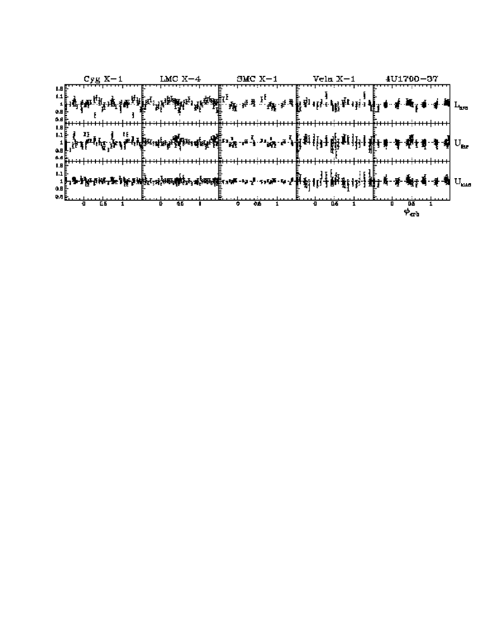
Figure 18: Lightcurves of the UV continuum flux and the UV colours as defined in the text.

To study variability in the spectrum tilt, we define UV colours in the following way:

$$U_{\rm far}=L_{1}-L_{2}\hskip 28.45274pt\&\hskip 28.45274ptU_{\rm mid}=L_{2}-L_{3}$$ (33)

where $L_{1}$, $L_{2}$ and $L_{3}$ are the fluxes (normalised to unity) for the wavelength bands 1, 2 and 3 in order of increasing wavelength. Because of the difficulty to find suitable wavelength bands of the best quality for each HMXB, the bands — and therefore the colours — are defined for each HMXB individually.

The UV continuum lightcurves are displayed in Fig. B1. The $L_{\rm ave}$ lightcurve is an average of all points within the 3 wavelength bands. It is not straightforward to determine the errors on the individual points in the lightcurve. The photometric accuracy of IUE is reported to be $\sim$6% at a 95% confidence level (Bohlin et al. 1980). This is probably a conservative estimate, judging from the small degree of scatter. For the error on the colour measurement we adopt the standard deviation of the distribution function of the measured $U_{\rm mid}$ points, which is a very conservative error estimate, and the same value is assigned to the error of the $U_{\rm far}$ colour.

B.1 HDE226868/Cyg X-1

The lightcurve of HDE226868/Cyg X-1 (Fig. B1) has a minimum to maximum amplitude of $\sim$17% (the deviating point at $\phi=0.281$ probably does not contain all the flux of the source). This is consistent with the scatter of similar amplitude in the UV photometry around 1500 and 1800 Å obtained by Wu et al. (1982) with the Astronomical Netherlands Satellite (ANS), but considerably larger than the 8% found by Treves et al. (1980) who analysed only 7 spectra by integrating the entire spectrum between 1250 and 1900 Å. The absence of X-ray eclipses limits the inclination to $i\sim 60\degr$ (Bolton 1975). Hence the deprojected amplitude is even larger, implying a severe deformation of HDE226868.

The U_far colour shows clear orbital modulation similar to the average flux: when the HMXB becomes fainter in the UV, the spectrum becomes redder. This may reflect a lower photospheric temperature of HDE226868 at the side that faces to and away from Cyg X-1, probably a result of the tidal deformation of the primary (Hutchings 1974). HDE226868 is possibly filling its tidal lobe during peri-astron of the slightly eccentric orbit ($e\sim 0.05$: Bolton 1975). No heating of the photosphere of the primary by the X-ray companion is observed, in agreement with Strömgren photometry by Hilditch & Hill (1974).

B.2 Sk-Ph/LMC X-4

The lightcurve of Sk-Ph/LMC X-4 (Fig. B1) has a minimum to maximum amplitude of $\sim$19%, and is an improvement over the lightcurve derived from only 15 spectra by van der Klis et al. (1982) (see also Vrtilek et al. 1997). The variable depth of the $\phi=0.5$ minimum was explained by a precessing accretion disk (van der Klis et al. 1982). The precession causes variations in the amount of surface of Sk-Ph that is exposed to X-ray heating, as well as variations in the fraction of Sk-Ph that is eclipsed by the disk. Heemskerk & van Paradijs (1989) confirmed the presence of an accretion disk that precesses with a period of 30.36$\pm 0.02$ days, whilst X-ray observations had already revealed a 30.42$\pm 0.03$ days period (Pakull et al. 1985); we adopt $P=30.38\pm 0.03$ days. Phase ${\phi}_{\rm prec}=0$ corresponds to the phase when the accretion disk is seen edge-on.

Figure 19: Continuum lightcurves of Sk-Ph/LMC X-4 for orbital phase bins as indicated in each of the nine frames. The cycle parameters are those of the precessing disk: $\phi_{0}\equiv$ JD 2 443 392.52(2); $P=30{\aas@@fstack{d}}38$(3). The dotted cosine waves are fits-by-eye to the data (see text).

Lightcurves are created according to the cycle parameters of the precession of the accretion disk, for bins around orbital phases ${\phi}_{\rm orb}=0$, 0.25 & 0.75, and 0.5 (Fig. B2). For orbital phases ${\phi}_{\rm orb}\sim 0$ no clear variability with the disk precession period is seen. For ${\phi}_{\rm orb}\sim 0.5$ the luminosity is lowest when the accretion disk eclipses the largest part of Sk-Ph (${\phi}_{\rm prec}=0.5$), and highest when the accretion disk is seen edge-on (${\phi}_{\rm prec}=0$). This is especially clear when narrower orbital phase bins are taken. At ${\phi}_{\rm orb}\sim 0.25$ & 0.75 the luminosity varies in anti-phase with the variation at ${\phi}_{\rm orb}=0.5$. Our results agree well with those of Heemskerk & van Paradijs (1989) from optical data. The amplitude of variability of the UV luminosity at ${\phi}_{\rm orb}=0.5$ is 10% — the same as in the optical.

The $U_{\rm far}$ colour (Fig. B1) is modulated with the orbital period. The colour behaviour around orbital phase ${\phi}_{\rm orb}\sim 0.5$ may be dominated by X-ray heating, causing the UV spectrum to become hotter close to ${\phi}_{\rm orb}=0.5$. The scatter in the U_far colour very close to ${\phi}_{\rm orb}=0.5$ may be due to variable obscuration by the precessing disk.

B.3 Sk 160/SMC X-1

The lightcurve of Sk 160/SMC X-1 (Fig. B1) has a minimum to maximum amplitude of $\sim$17%. In optical lightcurves the $\phi=0.5$ minimum is observed to be weaker than the $\phi=0$ minimum, explained by X-ray heating by the bright X-ray source (Hutchings 1974). Van Paradijs & Zuiderwijk (1977) and Howarth (1982), however, found that X-ray heating is not sufficient and that an emitting accretion disk is required, in agreement with the suggestion that the mass transfer is dominated by Roche-lobe overflow (Hutchings et al. 1977). Despite using more spectra than van der Klis et al. (1982), the orbital phase coverage of our UV lightcurve around $\phi=0.5$ is too poor to answer the question of X-ray heating and accretion disk. An $\sim 60$ day periodicity in the X-ray characteristics of SMC X-1 has been attributed to a precessing accretion disk (e.g. Wojdowski et al. 1998).

B.4 HD77581/Vela X-1

The lightcurve of HD77581/Vela X-1 (Fig. B1) has a minimum to maximum amplitude of $\sim$20% and clear orbital modulation, although Dupree et al. (1980) could not see continuum variability in the 5 low resolution spectra they used. The $\phi=0.5$ minimum is significantly deeper than the $\phi=0$ minimum, much alike the visual lightcurve (Zuiderwijk et al. 1977) that has a somewhat smaller amplitude of $\sim$15%. Zuiderwijk et al. argue that HD77581 is nearly filling its Roche lobe.

The $U_{\rm far}$ colour is modulated with the orbital period, becoming redder around $\phi=0.5$. This may be explained by temperature gradients over the photosphere of HD77581. The scatter of the $U_{\rm far}$ colour near $\phi=0.5$ may result from variable X-ray heating of the part of the photosphere of HD77581 that faces Vela X-1, due to the strongly variable X-ray flux.

B.5 HD153919/4U1700$-$37

The lightcurve of HD153919/4U1700$-$37 (Fig. B1) is flat within $\sim$4 to 5%, possibly with a marginable maximum at $\phi=0.5$. This is less than the UV amplitude around 1500 and 1800 Å of 8% found by Hammerschlag-Hensberge & Wu (1977) using the ANS. Optical amplitudes are $\sim$4 to 8% (Hammerschlag-Hensberge & Zuiderwijk 1977; van Paradijs et al. 1978). The small amplitude may be due to a large mass ratio of the system and therefore small distortion of HD153919. The optical lightcurve cannot be described by tidal distortion of HD153919 alone (van Paradijs et al. 1978). In particular the deepest minimum does not occur at $\phi=0.50$ but at $\phi=0.56$. Possible explanations include extra absorption originating from the mass flow in the system. The UV lightcurves presented here also suggest a minimum near $\phi=0.6$. Hints for the signature of a photo-ionization wake in Strömgren photometry are presented in Appendix C. The $U_{\rm far}$ colour is bluest at orbital phase $\phi=0.5$, which suggests X-ray heating of the part of the photosphere of HD153919 facing 4U1700$-$37.

Appendix C Strömgren $uvby\beta$ photometry of HD153919/4U1700$-$37

Figure 20: Strömgren $uvby$ photometry, the derived colours $m_{1}$ and $c_{1}$, and the $\beta$ parameter (see text) for HD153919/4U1700$-$37. The $uvby\beta$ are presented differentially with respect to the comparison star HD154368. Mean levels are represented by dotted lines.

In August 1993 we obtained Strömgren $uvby$ plus broad and narrow band H$\beta$ photometry using the 50 cm SAT at ESO/La Silla. The O9.5 Iab star HD154368 was measured for comparison. The photometry is presented in Tables C1 & C2. The magnitude differences between HD153919/4U1700$-$37 and HD154368 are plotted in Fig. C1, together with the colours $m_{1}$ and $c_{1}$ for HD153919/4U1700$-$37 as described in Sterken et al. (1995). The comparison star did not vary with time. The standard deviation for each individual measurement is typically 0.005 mag in $u$ and $y$, and 0.004 mag in $v$ and $b$. From the scatter on small orbital phase scales in the resulting lightcurves a formal, conservative estimate of 1-$\sigma\sim 0.01$ mag is derived. Because of the advantages of the multi-channel photometer, the errors in $m_{1}$ and $c_{1}$ are smaller than this. The standard deviation of the distribution of measured values gives an upper limit to the error on each individual measurement of 1-$\sigma=0.0065$ mag for both colours. The $\beta$ parameter is derived from the H$\beta$ narrow- and wide-band magnitudes. It increases with increasing absorption strength of the H$\beta$ line. The data give an upper limit to the error in $\beta$ of 1-$\sigma=0.0019$ mag.

Table 8: Heliocentric Reduced Julian Date RJD${}_{\odot}=$JD$-2\,449\,200$, $u$, $v$, $b$ and $y$ magnitudes (with their standard deviation of the last digit(s) within parentheses) and $\beta$ parameter of HD153919/4U1700$-$37. Orbital phases may be calculated from: $\phi_{0}\equiv$ JD 2 446 161.3400(30); $P=3{\aas@@fstack{d}}411652(26)$ (Haberl et al. 1989). The last row gives the mean values and their 1-$\sigma$ errors.

RJD⊙	$u$ (${\sigma}_{u}$)	$v$ (${\sigma}_{v}$)	$b$ (${\sigma}_{b}$)	$y$ (${\sigma}_{y}$)	$\beta$
09.6414	7.172(4)	7.071(3)	6.772(3)	6.584(4)	1.230
13.6344	7.153(4)	7.048(2)	6.751(2)	6.564(3)	1.249
14.6736	7.130(4)	7.023(3)	6.730(3)	6.544(4)	1.516
15.6159	7.086(2)	6.987(4)	6.695(3)	6.506(4)	1.195
16.6497	7.182(5)	7.078(3)	6.780(3)	6.595(5)	1.380
17.6424	7.101(5)	6.995(4)	6.703(4)	6.515(4)	1.352
18.5755	7.177(6)	7.067(4)	6.771(5)	6.594(6)	1.096
19.6214	7.114(5)	7.011(3)	6.717(3)	6.534(3)	1.268
20.6311	7.137(7)	7.036(4)	6.743(4)	6.556(4)	1.335
21.5959	7.155(3)	7.051(3)	6.755(3)	6.566(4)	1.183
22.5641	7.129(3)	7.025(2)	6.731(3)	6.541(3)	1.096
23.5721	7.187(7)	7.084(5)	6.784(4)	6.595(4)	1.124
24.5867	7.132(4)	7.025(4)	6.728(2)	6.539(3)	1.180
25.5770	7.183(7)	7.089(8)	6.787(8)	6.597(12)	1.158
26.5891	7.161(8)	7.052(3)	6.754(2)	6.566(5)	1.212
28.5688	7.141(3)	7.044(6)	6.748(7)	6.560(7)	1.159
32.5778	7.143(6)	7.042(3)	6.745(3)	6.554(3)	1.236
Aug’93	7.146(7)	7.043(7)	6.747(7)	6.559(7)	1.233(27)

Table 9: Same as Table C1, but now for the comparison star HD154368.

RJD⊙	$u$ (${\sigma}_{u}$)	$v$ (${\sigma}_{v}$)	$b$ (${\sigma}_{b}$)	$y$ (${\sigma}_{y}$)	$\beta$
09.6355	7.224(4)	6.962(2)	6.600(2)	6.151(2)	1.197
09.6475	7.224(4)	6.959(3)	6.598(2)	6.150(4)	1.250
13.6283	7.210(3)	6.946(2)	6.585(3)	6.139(2)	1.214
13.6405	7.207(5)	6.946(3)	6.584(2)	6.140(3)	1.271
14.6676	7.188(4)	6.928(3)	6.566(3)	6.124(3)	1.463
14.6795	7.186(7)	6.929(3)	6.567(3)	6.124(3)	1.566
15.6101	7.215(9)	6.949(5)	6.587(5)	6.139(3)	1.165
15.6237	7.207(4)	6.947(3)	6.583(2)	6.138(3)	1.219
16.6434	7.189(11)	6.927(5)	6.562(5)	6.116(5)	1.334
16.6560	7.182(4)	6.924(4)	6.560(5)	6.116(5)	1.418
17.6364	7.183(5)	6.918(4)	6.558(4)	6.112(4)	1.310
17.6484	7.177(6)	6.920(4)	6.558(4)	6.117(4)	1.384
18.5696	7.203(5)	6.931(4)	6.575(4)	6.142(5)	1.075
18.5832	7.209(6)	6.940(4)	6.582(4)	6.148(4)	1.107
19.6155	7.193(33)	6.933(8)	6.570(8)	6.127(6)	1.232
19.6283	7.185(6)	6.926(6)	6.567(5)	6.123(6)	1.296
20.6244	7.199(6)	6.933(4)	6.572(4)	6.126(4)	1.291
20.6374	7.192(6)	6.933(5)	6.572(4)	6.127(5)	1.368
21.5897	7.198(3)	6.939(2)	6.575(3)	6.127(3)	1.153
21.6021	7.206(6)	6.939(6)	6.575(5)	6.127(5)	1.199
22.5579	7.198(4)	6.935(3)	6.572(2)	6.124(2)	1.074
22.5707	7.195(3)	6.938(3)	6.574(3)	6.129(3)	1.104
23.5659	7.204(6)	6.938(5)	6.577(4)	6.129(4)	1.099
23.5784	7.197(4)	6.939(3)	6.576(3)	6.132(4)	1.134
24.5792	7.215(3)	6.956(2)	6.594(2)	6.148(3)	1.146
24.5931	7.213(4)	6.952(3)	6.592(2)	6.145(5)	1.197
25.5690	7.234(9)	6.972(7)	6.607(7)	6.158(7)	1.124
25.5837	7.236(12)	6.987(15)	6.622(15)	6.182(18)	1.172
26.5828	7.241(8)	6.975(5)	6.611(4)	6.161(4)	1.179
26.5956	7.230(6)	6.970(3)	6.607(3)	6.162(5)	1.231
28.5619	7.206(11)	6.948(4)	6.584(4)	6.137(4)	1.128
28.5756	7.204(4)	6.945(2)	6.582(2)	6.137(3)	1.173
32.5704	7.224(6)	6.969(4)	6.607(4)	6.164(6)	1.196
32.5859	7.210(8)	6.951(6)	6.589(7)	6.146(6)	1.266
Aug’93	7.205(3)	6.944(3)	6.582(3)	6.137(3)	1.228(20)

Our $uvby$ lightcurves of HD153919/4U1700$-$37 agree with the lightcurves obtained by Hammerschlag-Hensberge & Zuiderwijk (1977). They noticed an orbital modulation of the colour $m_{1}$, with a minimum at $\phi\sim 0.2$, and suggested that this might be caused by variability in the emission lines of He ii 4686, C iii 4650 and N iii 4634-4641 that are included in the Strömgren b-filter. Our observations indeed confirm a minimum in $m_{1}$ between $\phi=0.1$ and 0.2. Krzemiński (1976) did not find any orbital modulation of the He ii 4686 line. Kaper et al. (1994) found variability in the He ii 4686 line profile, but this alone cannot cause observable variability in the Strömgren b-filter. The other two mentioned emission lines may still be variable.

There is a weak indication for a gradual decrease in the H$\beta$ absorption (or an increase in emission) towards $\phi=1$, possibly with a secondary weak minimum around $\phi=0.3$ (Fig. C1). This is exactly what Kaper et al. (1994) found in their study of the variability in the H$\beta$ P-Cygni line profile. They attributed this to the presence of a photo-ionization wake.

Appendix D Covariances method for error and variability analysis

The degree of variability in a particular spectral point over a series of spectra can be expressed by the variance in that spectral point. The variances are often used to derive error estimates on the values of spectral points, and to detect intrinsic spectral variability. Usually two adjacent spectral points do not behave independently from eachother. Ignoring the covariability of adjacent spectral points can lead to serious under-estimation of the error on a quantity derived by integration along the spectrum. A correct error analysis therefore involves the calculation of covariances. Better than variances, covariances are powerful in detecting variability on an intermediate spectral scale — i.e. exceeding the instrumental profile but considerably smaller than the total spectral range. Covariances have also been used successfully in proving the reality of spectral features with low signal-to-noise (van Loon et al. 1996).

For a set of $N$ spectra, each consisting of a number of spectral values $x$, the covariance of points $a$ & $b$ is:

$$\sigma_{ab}^{2}=\frac{N\sum_{k=1}^{N}x_{ka}x_{kb}-(\sum_{k=1}^{N}x_{ka})(\sum_{k=1}^{N}x_{kb})}{N(N-1)}$$ (34)

It measures how much and how coherently the values of the two points vary from one spectrum to another. For $a=b$ the covariance reduces to the variance. Integrating the spectral values $x$ over a spectral range $(A,B)$ in spectrum $k$ yields:

$$I_{k}=\int_{A}^{B}x_{ki}{\rm d}i$$ (35)

with an error estimate $\sigma_{I_{k}}$ given by:

$$\sigma_{I_{k}}^{2}=\int_{A}^{B}\int_{A}^{B}\sigma_{ij}^{2}{\rm d}j{\rm d}i$$ (36)

Only if all points within $(A,B)$ behave statistically independently this reduces to the commonly used variance-deduced error estimate, because then:

$$\sigma_{ij}=\sigma_{ii}\delta_{ij}$$ (37)

with $\delta_{ij}$ the Kronecker delta function. In the opposite extreme when all points within $(A,B)$ behave in phase:

$$\sigma_{ij}=\sigma_{ii}$$ (38)

and consequently no increase in signal-to-noise can be obtained by integrating along the spectrum. The integrated covariances $\int_{A}^{B}\sigma_{ij}^{2}{\rm d}j$ are calculated in spectral regions without intrinsic spectral variability (Table D1) and tabulated in flux-wavelength space. Errors can then be assigned according to flux and wavelength. This assumes that the integrated covariances are a smooth function of flux and wavelength, which was proven to be true for IUE spectra (Howarth & Smith 1995).

Table 10: Intervals $(A,B)$, in Å, used for error estimation.

Cyg X-1	LMC X-4	SMC X-1	Vela X-1	4U1700$-$37
1250,1370	1170,1200	1250,1380	1153,1200	1183,1225
1420,1510	1280,1380	1415,1530	1253,1280	1420,1517
1565,1926	1430,1530	1560,1926	1315,1380	1730,1947
	1565,1926		1415,1530
			1565,1840

Figure 21: Covariance (top) and cumulative covariance (bottom) for Cyg X-1 (left) and Vela X-1 (right) as a function of distance along the spectrum with respect to the spectral point $i$. The drawn, dashed, dotted and dash-dotted lines represent the averages for the entire spectrum and the three spectral regions in which the continuum calibration factors were determined, respectively, with subsequently larger mean wavelength. The vertical long-dashed line indicates the choice of the integration boundary.

Figure 22: Variances (top) and integrated covariances (bottom) in the spectra of Cyg X-1 (left) and Vela X-1 (right), as a function of wavelength of the spectral points $i$.

The covariances $\sigma_{ij}^{2}$ decrease with increasing distance $|j-i|$ to the point $i$. If the integral of the covariances for the point $i$ converges sufficiently fast, then the integration interval $(A,B)$ in Eq. (D3) may be replaced by a smaller interval such that the integral of the covariances just reaches convergence. This interval is determined from a covariance profile of $\sigma_{ij}^{2}$ versus $j-i$, which represents the spectral shape of the instrumental profile. As an example the covariance profile and the cumulative covariance are shown for Cyg X-1 and Vela X-1 (Fig. D1). The dashed, dotted and dash-dotted lines represent the mean curves within the three regions in which the continuum calibration factors were determined (from shortest to longest wavelength, respectively), whilst the solid line represents the entire spectral range — i.e. including wildly variable spectral features. Both the covariance and the cumulative covariance at zero distance from the point $i$ reduce to the variance — i.e. the covariance of point $i$ with itself. At larger distances the covariance diminishes to a small oscillation around zero, whilst the initially rapidly growing cumulative covariance approximates a constant level.

For Cyg X-1 the solid line is too high to be captured within the frame of the plots, indicating that some parts of the spectrum are strongly variable. The width of the covariance profile corresponds to the specified spectral resolving power of about 250. The cumulative covariance indicates that a reasonable choice for the integration interval is $\pm 6$ Å. The sharp peak of the covariance profile of Vela X-1 indicates a spectral resolution in accordance with the specified spectral resolving power of about $10^{4}$. Its broad wings, however, prevent the cumulative covariance from converging within $\sim 16$ spectral points ($\equiv 1.6$ Å) — several times the specified spectral resolution.

Spectra of the variances and integrated covariances are shown for Cyg X-1 and Vela X-1 (Fig. D2) as an example of the detection of intrinsic spectral variability. In the low-resolution spectra of Cyg X-1 the spectral features (notably the Si iv and C iv resonance lines near 1400 and 1550 Å, respectively) and their variability are unresolved. The calculation of covariances does not improve the detection sensitivity much. In the high-resolution spectra of Vela X-1, however, the integrated covariance spectrum is much more sensitive than the variance spectrum in detecting intrinsic variability. Events that are limited to only one or very few adjacent pixels (like cosmics or dead pixels) cause a “forest” of sharp peaks in the variance spectrum, nearly completely obscuring the resolved but still narrow peaks of the intrinsic variability — the ”trees” of interest. By calculating the integrated covariance spectrum the forest is suppressed, and at the same time the features indicating intrinsic variability are enhanced. The variable spectral features can be identified easily.

References

- (1) Anders E., Grevesse N., 1989, Geochim.Cosmochim.Acta 53, 197
- (2) Blondin J.M., 1994, ApJ 435, 756
- (3) Bohlin R.C., Grillmair C.J., 1988, ApJS 66, 209
- (4) Bohlin R.C., Sparks W.M., Holm A.V., Savage B.D., Snijders M.A.J., 1980, A&A 85, 1
- (5) Bolton C.T., 1975, ApJ 200, 269
- (6) Bolton C.T., Herbst W., 1976, AJ 81, 339
- (7) Bondi H., Hoyle F., 1944, MNRAS 104, 273
- (8) Bonnet-Bidaud J.M., Ilovaisky S.A., Mouchet M., et al., 1981, A&A 101, 184
- (9) Boroson B., McCray R., Kallman T., Nagase F., 1996, ApJ 465, 940
- (10) Boroson B., Kallman T., McCray R., Vrtilek S.D., Raymond J., 1999, ApJ 519, 191
- (11) Boroson B., Kallman T., Blondin J.M., Owen M.P., 2001, ApJ 550, 919
- (12) Bregman J., Butler D., Kemper E., et al., 1973, ApJ 185, L117
- (13) Cassatella A., Selvelli P.L., Ponz J.D., Gonzalez-Riestra R., Vogel M., 1994, A&A 281, 594
- (14) Cassinelli J.P., Olson G.L., 1979, ApJ 229, 304
- (15) Castor J.I., 1970, MNRAS 149, 111
- (16) Chevalier C., Ilovaisky S.A., 1977, A&A 59, L9
- (17) Conti P.S., 1978, A&A 63, 225
- (18) Cowley A.P., Schmidtke P.C., Anderson A.L., McGrath T.K., 1995, PASP 107, 145
- (19) Davidson K., Ostriker J.P., 1973, ApJ 179, 585
- (20) Davis R., Hartmann L., 1983, ApJ 270, 671
- (21) Deeter J., Boynton P., Shibazaki N., et al., 1987, AJ 93, 877
- (22) Dupree A.K., Davis R.J., Gursky H., et al., 1978, Nat 275, 400
- (23) Dupree A.K., Gursky H., Black J.H., et al., 1980, ApJ 238, 969
- (24) Garmany C.D., Conti P.S., 1985, ApJ 293, 407
- (25) Giddings J.R., 1983, ESA IUE Newsletter 17, 53
- (26) González-Riestra R., Cassatella A., Solano E., Altamore A., Wamsteker W., 2000, A&AS 141, 343
- (27) Groenewegen M.A.T., Lamers H.J.G.L.M., 1989, A&AS 79, 359
- (28) Groenewegen M.A.T., Lamers H.J.G.L.M., 1991, A&A 243, 429
- (29) Groenewegen M.A.T., Lamers H.J.G.L.M., Pauldrach P.A.W., 1989, A&A 221, 78
- (30) Haberl F., White N.E., Kallman T.P., 1989, ApJ 343, 409
- (31) Hammerschlag-Hensberge G., Wu C.C., 1977, A&A 56, 433
- (32) Hammerschlag-Hensberge G., Zuiderwijk E.J., 1977, A&A 54, 543
- (33) Hammerschlag-Hensberge G., Kallman T.R., Howarth I.D., 1984, ApJ 283, 249
- (34) Hammerschlag-Hensberge G., Howarth I.D., Kallman T.R., 1990, ApJ 352, 698
- (35) Haser S.M., Pauldrach A.W.A., Lennon D.J., et al., 1998, A&A 330, 285
- (36) Hatchett S., McCray R., 1977, ApJ 211, 552
- (37) Hatchett S., Buff J., McCray R., 1976, ApJ 206, 847
- (38) Heap S.R., Corcoran M.F., 1992, ApJ 387, 340
- (39) Heemskerk M.H.M., van Paradijs J., 1989, A&A 223, 154
- (40) Hilditch R.W., Hill G., 1974, MNRAS 168, 543
- (41) Howarth I.D., 1982, MNRAS 198, 289
- (42) Howarth I.D., Prinja R.K., 1989, ApJS 69, 527
- (43) Howarth I.D., Smith K.C., 1995, ApJ 439, 431
- (44) Hutchings J.B., 1974, ApJ 193, L61
- (45) Hutchings J.B., Crampton D., Cowley A.P., Osmer P.S., 1977, ApJ 217, 186
- (46) Hutchings J.B., Crampton D., Cowley A.P., 1983, ApJ 275, L43
- (47) Hutchings J.B., Crampton D., Cowley A.P., Bianchi L., Thompson I.B., 1987, AJ 94, 340
- (48) Kallman T.R., McCray R., 1982, ApJS 50, 263
- (49) Kallman T.R., McCray R., Voit G.M., 1987, ApJ 317, 746
- (50) Kaper L., 1998, in: “Properties of Hot, Luminous Stars”, ed. I.D. Howarth, ASP Conf.Ser. 131, p427
- (51) Kaper L., 2001, in: “Influence of binaries on stellar population studies”, eds. D. Vanbeveren & W. van Rensbergen, Kluwer, in press
- (52) Kaper L., Hammerschlag-Hensberge G., Takens R.J., 1990, Nat 347, 652
- (53) Kaper L., Hammerschlag-Hensberge G., van Loon J.Th., 1993, A&A 279, 485
- (54) Kaper L., Hammerschlag-Hensberge G., Zuiderwijk E.J., 1994, A&A 289, 846
- (55) Kemp J.C., 1977, IAUC 3149
- (56) Krzemiński W., 1976, in: “X-ray Binaries”, NASA GSFC, p555
- (57) Kudritzki R.P., Pauldrach A., Puls J., 1987, A&A 173, 293
- (58) Lamers H.J.G.L.M., Cerruti-Sola M., Perinotto M., 1987, ApJ 314, 726
- (59) Lamers H.J.G.L.M., Snow T.P., Lindholm D.M., 1995, ApJ 455, 269
- (60) Lamers H.J.G.L.M., Haser S., de Koter A., Leitherer C., 1999, ApJ 516, 872
- (61) Levine A., Rappaport S., Putney A., Corbet R., Nagase F., 1991, ApJ 381, 101
- (62) Lewin W.H.G., van Paradijs J., van den Heuvel E.P.J. (eds.), “X-ray binaries”, 1995, Cambridge University Press
- (63) Lucy L.B., 1982, ApJ 255, 278
- (64) Masai K., 1984, Ap&SS 106, 391
- (65) McCray R., Kallman T.R., Castor J.I., Olson G.L., 1984, ApJ 282, 245
- (66) Nagase F., 1989, PASJ 41, 1
- (67) Osmer P.S., 1973, ApJ 181, 327
- (68) Owocki S.P., 1994, Ap&SS 221, 3
- (69) Pakull M., Brunner H., Staubert A., Pietsch W., Beuermann K., 1985, Space Science Reviews, vol. 40, p379
- (70) Payne B.J., Coe M.J., 1987, MNRAS 225, 985
- (71) Prinja R.K., 1987, MNRAS 228, 173
- (72) Prinja R.K., Barlow M.J., Howarth I.D., 1990, ApJ 361, 607
- (73) Rappaport S., Joss P.C., 1983, in: “Accretion-driven stellar X-ray sources”, eds. W.H.G. Lewin & E.P.J. van den Heuvel, Cambridge University Press, p13
- (74) Reynolds A.P., Owens A., Kaper L., et al., 1999, A&A 349, 873
- (75) Sadakane K., Hirata R., Jugaku J., et al., 1985, ApJ 288, 284
- (76) Shakura N.I., Sunyaev R.A., 1973, A&A 24, 337
- (77) Sterken C., Manfroid J., Beele D., et al., 1995, A&AS 113, 31
- (78) Tarter C.B., Tucker W.H., Salpeter E.E., 1969, ApJ 156, 943
- (79) Treves A., Chiappetti L., Tanzi E.G., et al., 1980, ApJ 242, 1114
- (80) van der Klis M., Hammerschlag-Hensberge G., Bonnet-Bidaud J.M., et al., 1982, A&A 106, 339
- (81) van Loon J.Th., 2000, A&A 354, 125
- (82) van Loon J.Th., Zijlstra A.A., Bujarrabal V., Nyman L.-Å., 1996, A&A 306, L29
- (83) van Paradijs J., 1998, in: “The Many Faces of Neutron Stars”, eds. R. Buccheri, J. van Paradijs & M.A. Alpar, Kluwer, Dordrecht, p279
- (84) van Paradijs J., Kuiper L., 1984, A&A 138, 71
- (85) van Paradijs J., Zuiderwijk E., 1977, A&A 61, L19
- (86) van Paradijs J., Hammerschlag-Hensberge G., Zuiderwijk E.J., 1978, A&AS 31, 189
- (87) Vrtilek S.D., Boroson B., Cheng F.H., McCray R., Nagase F., 1997, ApJ 490, 377
- (88) Walborn N.R., 1973, AJ 78, 1067
- (89) Webster B., Martin W., Feast M., Andrews P., 1972, Nature Phys.Sci. 240, 183
- (90) White N.E., Marshall F.E., 1983, IAUC 3806, 2
- (91) Wojdowski P., Clark G.W., Levine A.M., Woo J.W., Zhang S.N., 1998, ApJ 502, 253
- (92) Wu C.-C., Eaton J.A., Holm A.V., Milgrom M., Hammerschlag-Hensberge G., 1982, PASP 94, 149
- (93) Zuiderwijk E.J., Hammerschlag-Hensberge G., van Paradijs J., Sterken C., Hensberge H., 1977, A&A 54, 167