The dust temperature distribution in prestellar cores

We have computed the dust temperature distribution to be expected in a pre–protostellar core in the phase prior to the onset of gravitational instability. We have done this in the approximation that the heating of the dust grains is solely due to the attenuated external radiation field and that the core is optically thin to its own radiation. This permits us to consider non spherically symmetric geometries. We predict the intensity distributions of our model cores at millimeter and sub–millimeter wavelengths and compare with observations of the well studied object L1544. We have also developed an analytical approximation for the temperature at the center of spherically symmetric cores and we compare this with the numerical calculations. Our results show (in agreement with Evans et al. 2001) that the temperatures in the nuclei of cores of high visual extinction ($>$ 30 magnitudes) are reduced to values of below $\sim 8$ K or roughly half of the surface temperature. This has the consequence that maps at wavelengths shortward of 1.3 mm see predominantly the low density exterior of pre–protostellar cores. It is extremely difficult to deduce the true density distribution from such maps alone. We have computed the intensity distribution expected on the basis of the models of Ciolek & Basu (2000) and compared with the observations of L1544. The agreement is good with a preference for higher inclinations (37^∘ instead of $16^{\circ}$ ) than that adopted by Ciolek & Basu (2000). We find that a simple extension of the analytic approximation allows a reasonably accurate calculation of the dust temperature as a function of radius in cores with density distributions approximating those expected for Bonnor–Ebert spheres and suggest that this may be a useful tool for future calculations of the gas temperature in such cores.

1 Introduction

The structure of the high density cores embedded in nearby molecular clouds is currently a matter of great interest. The fate of a protostar depends sensitively on the initial conditions prior to collapse and it is difficult to infer this from studies of “protostars” where a luminous object has already formed. Considerable observational effort has therefore been expended in the attempt to detect a “pre-protostellar core”, which is taken to be a cold dense core whose column density and internal pressure exceed considerably those found in the surroundings. The high density nucleus of the dark cloud L1544 is an example of such an object (Tafalla et al. 1998, Ward–Thompson et al. 1999, Williams et al. 1999, Ciolek & Basu 2000a,b) and in fact the models of Ciolek & Basu (2000a, CB hereafter) suggest that it will become unstable in around 30000 years from now. However, these inferences depend on our ability to derive the density distribution in such sources from observables such as the millimeter emission and the mid–IR absorption (e.g. Bacmann et al. 2000).

In particular, the emission of dust grains at millimeter and submillimeter wavelengths is sensitively dependent not only on the grain column density but also upon the grain temperature. In clouds such as L1544, the grain temperature is known to be of order 12 K on the basis of the observed spectral energy distribution (André et al. 2000) and it has been normal practise to assume such regions to be isothermal. However, it has been known for some time that one can expect appreciable temperature gradients within cores heated by the (external) interstellar radiation field (e.g. Leung 1975; Mathis et al. 1983, hereafter MMP) as well as temperature differences between grains of differing optical properties. For example, for silicate grains, MMP predict grain temperatures as low as 6 K in the nucleus of cores of visual extinction $\sim$ 50 magnitudes. Such low temperature grains will contribute negligibly to the emission at wavelengths below 1 mm and this suggests that a new study of grain temperatures in dense cloud cores similar to L1544 is warranted.

Another characteristic of the observed pre–protostellar cores is that they clearly show large departures from spherical symmetry in both the maps of dust emission and absorption (Bacmann et al. 2000). This is often interpreted as being due to flattening along the direction of the mean magnetic field resulting in a disk-like configuration (Ciolek & Basu 2000a,b). Furthermore, as shown recently by Galli et al. (2001), a cloud core modeled as a thin disk perpendicular to the large-scale magnetic field and supported against its self-gravity by a combination of gas pressure and magnetic forces, is not necessarily axisymmetric. Direct evidence for the importance of a magnetic field in determining the structure of L1544 comes both from polarization measurements at 850 $\mu\hbox{m}$ (Ward–Thompson et al. 2000) and observation of OH Zeeman splitting (Crutcher & Troland 2000). The magnetic field inferred from the Zeeman measurement is consistent with the model predictions of CB but this result is sensitive to the assumed inclination of the magnetic field relative to the plane of the sky (16^∘, according to CB). It is relevant also that the observed direction of polarization is not consistent with naive CB model expectations in that the inferred magnetic field direction in the plane of the sky deviates by an angle of 30^∘ from that expected (parallel to the L1544 minor axis). This can be easily explained if the cloud is slightly non-axisymmetric (Basu 2000, Galli et al. 2001). Thus, while it seems plausible that the magnetic field plays an important role in the evolution of pre–protostellar cores just prior to collapse, it is possible that the “standard” ambipolar diffusion model requires modification. One notes however that the effects of temperature gradients mentioned earlier will have the qualitative effect of biasing the 850 $\mu\hbox{m}$ polarization measurements towards the lower density outer parts of cores such as L1544. Thus it is clearly of importance to be able to assess how large such temperature gradients really are.

With this in mind, we report here new calculations of the expected temperature distribution in pre–protostellar cores. We note that a rather similar study has recently been carried out by Evans et al. (2001, hereafter ERSM). These authors have confined themselves to models with spherical symmetry and have compared their model predictions to the observations of Shirley et al. (2000). We, in contrast, have employed a technique which allows us to simulate non spherically symmetric situations such as the magnetic field dominated models mentioned earlier. We however concur with ERSM in their conclusion that the decrease of temperature towards the centers of cores strongly affects the observed sub–millimeter emission. We also use our models to predict the emission distribution expected on the basis of the CB models and conclude that a reasonable fit to the observations can be obtained.

The structure of this paper is as follows. In section 2, we describe the model which we have used and the assumptions which we have made. In section 3, we present an analytic treatment aimed at determining the dust temperature at the center of a spherically symmetric cloud. In section 4, we give numerical results for both spherically symmetric models and models based on the density distributions of the CB models. Then, in section 5, we consider the intensity distributions which would be expected for mm–submm maps of our model cores and compare with observed data. In section 6, we summarize our conclusions.

2 Model

Our model calculations are aimed at calculating grain temperatures under physical conditions similar to those thought to pertain in L1544 and similar pre–protostellar cores. We have made a number of simplifying assumptions in doing this which we justify in the following discussion. One of these is that we neglect scattering as we are interested in studying cores of more than 10 magnitudes of visual extinction which are mainly penetrated by the external infrared interstellar radiation field for which the Rayleigh limit holds and thus scattering becomes negligible.

Another important assumption which we make is that grains are only heated by the incident radiation field and that other sources of grain heating are negligible. ERSM provide a detailed discussion of the range of applicability of this and conclude that for representative conditions with dust grain temperatures above 5 K, heating due to the ambient radiation field dominates. We follow them in this but differ from them in only considering heating due to the (attenuated) external radiation field. That is to say, we assume that our model cores are optically thin to their own radiation and that we can neglect re–absorption of radiation emitted from within our model itself. This is an essential simplification which permits us to consider non spherically symmetric geometries. However, it restricts us to considering structures with hydrogen column densities less than a few hundred visual magnitudes of extinction.

The rationale behind this can be understood if one notes that for typical temperatures of order 10 K, one expects the bulk of the emission from a pre–protostellar core such as L1544 at wavelengths of order 200–300 $\mu\hbox{m}$. The available observations (see André et al. 2000 for the case of L1544) fully confirm this. Then to maintain the optical depth below, say, 0.1 at 200 $\mu\hbox{m}$ requires a column density of ${\rm H_{2}}$ less than $5\times 10^{23}$ $\hbox{{\rm cm}}^{-2}$ corresponding to roughly 500 magnitudes of visual extinction. Available observational data suggest that this condition is satisfied in all cases. We note however that for models with a singularity at the origin such as the singular isothermal sphere of Shu (1977), this condition is strictly speaking not fulfilled.

We determine the grain temperature at a given position simply by applying the “classical” equilibrium between grain cooling and heating for a spherical grain at position $r$ in the dust cloud (see e.g. Spitzer 1978 or Boulanger et al. 1998 for a discussion),

$$\int^{\infty}_{0}Q_{\nu}B_{\nu}[T_{\rm d}(r)]\;d\nu=\int^{\infty}_{0}Q_{\nu}J_{\nu}(r)\;d\nu.$$ (1)

Here, the right hand side describes the grain heating due to an incident radiation field of average intensity $J_{\nu}(r)$ upon grains of absorption efficiency $Q_{\nu}$ at frequency $\nu$. The left hand side gives the cooling rate for a grain of temperature $T_{\rm d}(r)$ and $B_{\nu}$ is the Planck function.

The only real computational difficulty here is posed by the incident radiation field $J_{\nu}(r)$ which we suppose to be given by the attenuated interstellar radiation field $J_{\nu}^{\rm is}$. Thus, we have :

$$J_{\nu}(r)=\frac{J_{\nu}^{\rm is}}{4\pi}\int\exp[-\tau_{\nu}(r,\theta,\phi)]\;d\Omega$$ (2)

Here, the integral over solid angle describes the average attenuation due to an optical depth $\tau_{\nu}(r,\theta,\phi)$ in any given direction.

In order to compute grain temperature for a model cloud of relatively arbitrary geometry, one thus must find an efficient method of performing the angle integration of equation 2. Once the grain temperature is determined for all positions, a simple integral allows one to derive the intensity distribution expected at a given wavelength. One merely needs to choose the incident interstellar radiation field $J_{\nu}^{\rm is}$ and the grain absorption efficiency $Q_{\nu}$.

There are a number of choices which one can make concerning the grain opacities. Mathis (1990) has tabulated values expected for “standard” interstellar grains and we have used these for comparison purposes. However, within dense dust clouds, one expects grains to acquire ice mantles and this will substantially change their optical properties. In addition, one expects at the densities of interest to us that grain coagulation may change the size distribution. We have therefore used for many purposes the opacities computed by Ossenkopf & Henning (1994, hereafter OH) for grains which have coagulated for a time of $10^{5}$ years. As a standard case, we have used their case for thin ice mantles and density $10^{6}$ $\hbox{{\rm cm}}^{-3}$  but we note that in many situations, it is more realistic for pre–protostellar cores to consider their “thick ice mantle case”. We have found however that for our purposes, the difference between the two is not great as is the difference between their solutions for different densities. This is consistent with the fact that Kramer et al. (1997) find that the observed ratio of infrared extinction to millimeter emissivity in IC5146 (for visual extinctions in the range 20-30 magnitudes) is compatible with the OH results.

In similar fashion, we have used as a comparison standard the solar neighbourhood radiation field given by MMP. Black (1994) has updated this work using results from the FIRAS experiment on COBE (Wright et al. 1991). This suggests that the MMP field is an underestimate in the mid and far IR . However, in any case, the values used are an “educated” guess concerning the field actually incident upon cores such as L1544 and one can expect differences from one region to another. For example, it is clear that small particle emission in the mid infrared can be an important component of the incident radiation field and one expects this to depend on the far ultra–violet radiation from neighbouring O-B stars. This can be expected to vary depending on how many massive stars have formed in the vicinity of a given core. One notes from the work of Bacmann et al. (2000, their table 1) that the intensity in the LW2 ISOCAM filter (5-8.5$\mu\hbox{m}$) is 0.6 MJy/sr towards L1544 in Taurus (a factor of order 3 larger than the average radiation field at this wavelength according to Black (1994)) but 20.6 MJy/sr towards the OphD core (after correcting for zodiacal light). This seems likely to be typical also of the small particle radiation at wavelengths up to 50$\mu\hbox{m}$.

Finally, we need to define the density distribution of our models. For spherically symmetric cases, we have used the following density distributions: (i) a homogeneous sphere, (ii) a Bonnor-Ebert sphere (Bonnor 1956, Ebert 1955), and (iii) a singular isothermal sphere (Chandrasekhar 1939, Shu 1977). Case (i) was chosen to test the accuracy of the numerical scheme, since in this simple case exact solutions for the mean intensity and analytical approximations for the dust temperature are easily derived. Cases (ii) and (iii) represent equilibria of self-gravitating non-magnetized isothermal clouds and have been extensively adopted to model the density profiles of pre-protostellar cores. Notice that in cases (ii) and (iii) the structure of the cloud is computed assuming that the gas is isothermal. However, the dust clearly is not. Moreover in the central parts of the core at densities above $10^{5}$ $\hbox{{\rm cm}}^{-3}$, the gas and dust temperatures are likely to be coupled (see e.g. Goldsmith 2001) and hence there is strictly speaking an inconsistency which we will ignore in the following discussion. It is however a point which requires further study.

In all cases (including the non spherically symmetric models discussed below), the model “core” was truncated at an outer radius $R_{\rm out}$, and embedded in an envelope of radius $R_{\rm env}$ and uniform density $\rho_{\rm env}$, equal to the density of the cloud at radius $R_{\rm out}$. The rationale of this is that it simulates the “outer skin” of the molecular cloud where a PDR (Photon dominated region) shields the molecular gas against UV and is consistent with the idea that the internal molecular cloud pressure should not fall below the average interstellar pressure. Thus, the value of $\rho_{\rm env}$ was chosen to simulate the effect of the internal GMC pressure $P_{G}$ confining the core. One expects $P_{G}$ to be a factor of a few larger than the mean ISM pressure of roughly $2\times 10^{4}$ K $\hbox{{\rm cm}}^{-3}$(see section 2 of McKee 1999). If we take $P_{G}$ equal to this minimum value and assume a typical line width of 1 ${\rm km\thinspace s}^{-1}$  we find an envelope density corresponding to $n_{\rm H_{\rm 2}}$ = 1000 $\hbox{{\rm cm}}^{-3}$. This outer PDR layer should provide shielding equivalent to 1 magnitude of visual extinction and we define $R_{\rm env}$ such that $n_{\rm H_{\rm 2}}\,(R_{\rm env}-R_{\rm out})\,=\,1\times 10^{21}$ $\hbox{{\rm cm}}^{-2}$. We note that while these assumptions are somewhat ad hoc, they have little influence on our results which concern the high density core where the extinction is much higher than 1 magnitude.

Our non spherically symmetric models are based on the results of CB who have studied the development of infall driven by ambipolar diffusion assuming axial symmetry. They present results for a “disk–like” model and give the mid–plane density as a function of radius at times $t_{j}$ ($j=0$,1,2,3…) when the central density $n_{c}(t_{j})\,=\,10^{j}\,n_{c0}$ with $n_{c0}=4.4\times 10^{3}$ $\hbox{{\rm cm}}^{-3}$. The times $t_{j}$ are 0, 2.27, 2.60, 2.66, 2.68 … Myr from which one sees that the last stages of the evolution are extremely rapid. In this study, we consider the density distributions at times $t_{2}$, $t_{3}$, and $t_{4}$ as being of most interest from the standpoint of comparison with data for cores similar to L1544. We also need to make an assumption about the density distribution in the direction perpendicular to the disk midplane. We have assumed that hydrostatic equilibrium is valid in the $z$ direction (perpendicular to the mid–plane) and hence that the density can be expressed as $n(r,z)\,=\,n_{c}(t_{j})F_{CB}(r)\phi(z)$ with $F_{CB}(r)$ taken from the study of CB and $\phi(z)=\,1/\cosh^{2}(z/H)$ where the scale height is $H=[kT/(2\pi{\rm G}\rho)]^{1/2}$ and $\rho$ is the density. For this purpose, the disk is considered to be isothermal at a temperature of 12 K. Again, this is certainly not self–consistent for the reasons mentioned earlier but this seems a reasonable approximation to the density distribution of a CB model.

3 Analytical results for spherically symmetric clouds

The results for spherically symmetric models are important to us both because they can be treated to some extent with analytic techniques and because direct comparisons are possible with ERSM. As a check on our computational accuracy, we first show our results for the mean intensity in a homogeneous spherical cloud compared with the analytic solution.

3.1 Mean intensity in a homogeneous sphere

The solution of the full equation of radiative transfer in a homogeneous sphere can be obtained analytically with the spherical harmonics method (Flannery, Roberge, & Rybicki 1980). In Appendix A we show that for a homogeneous cloud of radius $R$ and centre-to-edge optical depth $\tau_{\nu c}$, the calculation of $J_{\nu}(r)$ from eq. (2) is straightforward and can be expressed in terms of exponential-integral functions of the argument $x_{\pm}=\tau_{\nu c}(1\pm x)$, where $x=r/R$:

$$J_{\nu}(x)=\frac{J^{\rm is}_{\nu}}{2(x_{+}-x_{-})}\times$$ (3)

$$\left[x_{+}E_{2}(x_{-})-x_{-}E_{2}(x_{+})+x_{-}E_{0}(x_{-})-x_{+}E_{0}(x_{+})\right].$$

Approximate expressions for the mean intensity can be obtained in the limit of very large or very small $\tau_{\nu c}$. In the optically thin limit eq. (3) becomes

$$J_{\nu}(x)\simeq J^{\rm is}_{\nu}\left\{1-\tau_{\nu c}\left[\frac{1}{2}+\frac{1-x^{2}}{4x}\ln\left(\frac{1+x}{1-x}\right)\right]\right\},$$ (4)

whereas an approximate formula (diverging for $x\rightarrow 1$) for the optically thick case is

$$J_{\nu}(x)\simeq J^{\rm is}_{\nu}\frac{e^{-\tau_{\nu c}}}{2\tau_{\nu c}x}\left(\frac{e^{\tau_{\nu c}x}}{1-x}-\frac{e^{-\tau_{\nu c}x}}{1+x}\right).$$ (5)

In Figure 1, we compare the exact and approximate analytical results with that obtained numerically integrating eq. (2). We see that the numerical code reproduces the analytic result very well. Thus, in simple geometries, the procedure used for the angle integration is adequate.

Figure 1: Mean intensity $J_{\nu}$ for a homogeneous spherical cloud as a function of radius $x=r/R$ computed by numerical integration of eq. (2) (solid lines) compared with the analytic formula eq. (3) (triangles). The approximated expressions (4) and (5) for the optically thin and thick cases are shown by dashed lines. Results are shown for two model clouds with $\tau_{\nu c}=0.1$ and 10.

3.2 The dust temperature at the centre of a spherical cloud

There are great advantages in developing analytic formulae which allow an approximate estimate of the temperature in dense pre–protostellar cores. This permits for example a discussion of scaling relationships for different external radiation fields and opacities. We have accordingly attempted to derive an analytical estimate of the temperature at the center of a spherically symmetric cloud for comparison with our numerical results.

In order to develop an analytic approximation, we must first make some crude approximations concerning the dust opacity and external radiation field in cores such as L1544. Following Black (1994) and MMP, the interstellar radiation field at wavelengths above 0.1 $\mu$m can be represented by the sum of four contributions: (1) an optical-NIR component peaking at $\lambda_{\rm p}=1$ $\mu$m, due to the emission of disk dwarf and giant stars; (2) the diffuse FIR emission from dust grains, peaking at $\lambda_{\rm p}=100$ $\mu$m; (3) mid–IR radiation from small non–thermally heated grains in the range 5–100 $\mu\hbox{m}$ and (4) the cosmic background radiation, peaking at $\lambda_{\rm p}=1$ mm. Components 1,2, and 4 can be represented by a single (or a sum of) modified black-bodies at temperatures $T_{i}$ of the kind

$$J_{\nu}^{\rm is}=\frac{2h\nu^{3}}{c^{2}}\left(\frac{\lambda_{\rm p}}{\lambda}\right)^{p}\sum_{i}\frac{W_{i}}{e^{h\nu/kT_{i}}-1},$$ (6)

where $\lambda_{\rm p}$ is the peak wavelength and $W_{i}$ are dilution factors. The values of the parameters $\lambda_{\rm p}$, $W_{i}$ and $T_{i}$ are listed in Table 1. The third (MIR) component is found to be variable near dense cores such as L1544 and can be approximated as a power law. In the following discussion however, we at first neglect it and then make an estimate of its importance.

As in the numerical computations, we have based our opacity law on the work of OH (thin ice, density $10^{6}$ $\hbox{{\rm cm}}^{-3}$). For the purposes of our analytic work, a very crude piecewise power law fit with breaks at 10 $\mu\hbox{m}$ and 400 $\mu\hbox{m}$ has been used (see Table 2). We then assume that in a sufficiently large range of wavelengths around the peak of each component, the dust absorption efficiency $Q_{\nu}$ can be approximated by a power-law, $Q_{\nu}\propto(\lambda_{\rm p}/\lambda)^{\alpha}$. The values of the parameters $\lambda_{\rm p}$ and $\alpha$ used by us are listed in Table 2.

Let the radiation absorbed (indicated by the subscript “a”) by dust be concentrated around a frequency $\nu_{a}$, and the radiation emitted (indicated by the subscript “e”) by dust be characterized by a frequency $\nu_{e}$. We take $\nu_{e}$ and $\alpha_{e}$ equal to the values for absorption in the FIR (see Table 2), and we consider the heating of the dust by each component of the radiation field separately.

With these assumptions, the mean intensity at the cloud’s center is

$$J_{\nu}(0)=J_{\nu}^{\rm is}\exp{(-\tau_{\nu c})}=J_{\nu}^{\rm is}\exp{\left[-\tau_{a}\left(\frac{\nu}{\nu_{a}}\right)^{\alpha_{a}}\right]},$$ (7)

where $\tau_{a}$ is the centre-to-edge optical depth of the cloud at frequency $\nu_{a}$. Then, defining $\beta_{d}\equiv kT_{d}/h\nu_{e}$, $\beta_{i}\equiv kT_{i}/h\nu_{a}$, eq. (1) becomes

$${\cal A}=\frac{Q_{a}}{Q_{e}}\left(\frac{\nu_{a}}{\nu_{e}}\right)^{4}\left(\frac{\nu_{a}}{\nu_{\rm p}}\right)^{p}\sum_{i}W_{i}{\cal B}_{i},$$ (8)

where $Q_{a}$ and $Q_{e}$ are the values of $Q_{\nu}$ at frequencies $\nu_{a}$ and $\nu_{e}$, respectively, and

$${\cal A}=\int_{0}^{\infty}\frac{t^{\alpha_{e}+3}}{e^{t/\beta_{d}}-1}\;dt=\Gamma(\alpha_{e}+4)\zeta(\alpha_{e}+4)\beta_{d}^{\alpha_{e}+4},$$ (9)

$${\cal B}_{i}=\int_{0}^{\infty}\frac{t^{q}}{e^{t/\beta_{i}}-1}\exp{(-\tau_{a}t^{\alpha_{a}})}\;dt,$$ (10)

with $q=\alpha_{a}+p+3$. In the above, $\Gamma$ and $\zeta$ are the gamma and Riemann zeta functions (see Abramovitz & Stegun 1965). The integral in the equation for ${\cal B}_{i}$ can be easily evaluated in the two limiting situations $\tau_{a}\ll 1$ and $\tau_{a}\gg 1$. For $\tau_{a}\ll 1$ the exponential in ${\cal B}_{i}$ can be expanded as a Taylor series, giving, to first order in $\tau_{a}$,

$${\cal B}_{i}\simeq\Gamma(q+1)\zeta(q+1)\beta_{i}^{q+1}$$ (11)

$$-\tau_{a}\Gamma(q+\alpha_{a}+1)\zeta(q+\alpha_{a}+1)\beta_{i}^{q+\alpha_{a}+1}+\ldots.$$

Thus, the dust temperature at the center is given, to lowest order, by

$$\frac{kT_{d}}{h\nu_{e}}\simeq C\left(\sum_{i}W_{i}\beta_{i}^{q+1}\right)^{\frac{1}{\alpha_{e}+4}},$$ (12)

where

$$C=\left[\frac{\Gamma(q+1)\zeta(q+1)}{\Gamma(\alpha_{e}+4)\zeta(\alpha_{e}+4)}\frac{Q_{a}}{Q_{e}}\left(\frac{\nu_{a}}{\nu_{e}}\right)^{4}\left(\frac{\nu_{a}}{\nu_{p}}\right)^{p}\right]^{\frac{1}{\alpha_{e}+4}}.$$ (13)

We note here that for the case of interest in which the dust is heated by (optically thin) FIR radiation, $Q_{a}=Q_{e}$, $\nu_{a}=\nu_{p}=\nu_{e}$ and one finds that $C\simeq 1.68$ is a constant slightly dependent on the power law index of the dust opacity but otherwise independent of dust characteristics.

For $\tau_{a}\gg 1$ the integrand in ${\cal B}_{i}$ can be expanded as a Taylor series for small $t$, obtaining the approximate result

$${\cal B}_{i}\simeq\frac{\beta_{i}}{\alpha_{a}}\Gamma\left(\frac{q}{\alpha_{a}}\right)\tau_{a}^{-q/\alpha_{a}}$$ (14)

$$-\frac{1}{2\alpha_{a}}\Gamma\left(\frac{q+1}{\alpha_{a}}\right)\tau_{0}^{-(q+1)/\alpha_{a}}+\ldots.$$

Thus, the dust temperature at the center is given, to lowest order, by

$$\frac{kT_{d}}{h\nu_{e}}\simeq D\tau_{a}^{-q/[(\alpha_{e}+4)\alpha_{a}]}\left(\sum_{i}W_{i}\beta_{i}\right)^{\frac{1}{\alpha_{e}+4}},$$ (15)

where

$$D=\left[\frac{\Gamma(\frac{q}{\alpha_{a}})}{\alpha_{a}\Gamma(\alpha_{e}+4)\zeta(\alpha_{e}+4)}\frac{Q_{a}}{Q_{e}}\left(\frac{\nu_{a}}{\nu_{e}}\right)^{4}\left(\frac{\nu_{a}}{\nu_{p}}\right)^{p}\right]^{\frac{1}{\alpha_{e}+4}}.$$ (16)

Notice that the dependence of the dust temperature on the intensity of the external radiation is rather weak, $T_{d}\propto W^{1/(\alpha_{e}+4)}$. Again, this expression simplifies considerably when the dust is heated by (optically thick) FIR radiation, and $D\simeq 0.59$ in this case.

The above discussion has neglected the contribution of the MIR radiation. We approximate the external MIR field with a power law spectrum in the wavelength range 10–100 $\mu\hbox{m}$ and with a lower frequency cut–off at 100$\mu\hbox{m}$,

$$J_{\nu}^{\rm is}=W\frac{2h\nu_{p}^{3}}{c^{2}}\left(\frac{\nu}{\nu_{p}}\right)^{p},$$ (17)

with the values of $W$, $\lambda_{p}$ and $p$ given in Table 1. Notice that $p<0$ in this case and thus for the “MIR” radiation, there is approximate cancellation in the integral on the right hand side of equation  1 between the frequency dependence of $Q_{\nu}$ and that of the external MIR field. The consequence is that the main contribution to the integral comes from frequencies where the optical depth is of order unity (i.e. at a wavelength of roughly 20$\mu\hbox{m}$ for $A_{V}$=30 mag.).

Substituting the above expression for the MIR field in eq. (1), we obtain

$${\cal A}=W\left(\frac{\nu_{p}}{\nu_{a}}\right)^{4}\frac{\Gamma(s,\tau_{a})}{\alpha_{a}}\tau_{a}^{-s},$$ (18)

where $s=(\alpha_{a}+p+1)/\alpha_{a}\,=\,0.5$ for our parameters, and $\Gamma(s,\tau_{a})$ is the incomplete gamma function. Here $\tau_{a}$ is the cloud’s optical depth at 100 $\mu\hbox{m}$, which becomes unity at $A_{V}\simeq 414$. Below this value, the incomplete gamma function can be expanded for small $\tau_{a}$, obtaining

$$\Gamma(s,\tau_{a})\simeq\Gamma(s)+\frac{\tau_{a}^{s}}{s}-\frac{\tau_{a}^{s+1}}{s+1}+\ldots.$$ (19)

In eq. (12), (15), (18) and (19), it is convenient to express the optical depth $\tau_{a}$ in terms of the optical extinction $A_{V}$,

$$A_{V}=1.086\tau_{V}=1.086\left(\frac{Q_{V}}{Q_{a}}\right)\tau_{a},$$ (20)

where the ratio in parentheses can be computed for each components with the parameters listed in Table 2 for the Ossenkopf & Henning (1994) opacity. We see that a cloud is optically thin to V-NIR radiation for $A_{V}\ll 3$, to FIR radiation for $A_{V}\ll 700$, and to the cosmic background radiation for $A_{V}\ll 6\times 10^{4}$. Thus, with Black (1994) standard interstellar field, the central temperature in a “diffuse” cloud core of typical centre-to-edge extinction $A_{V}\simeq 1$–2 is determined by optically thin absorption of V-NIR and MIR radiation (the effects of an external UV field are not considered here) whereas for $10\mathbin{\lower 3.0pt\hbox{$\hbox to0.0pt{\raise 5.0pt\hbox{$\char 60\relax$}\hss}\mathchar 29208\relax$}}A_{V}\mathbin{\lower 3.0pt\hbox{$\hbox to0.0pt{\raise 5.0pt\hbox{$\char 60\relax$}\hss}\mathchar 29208\relax$}}400$ is determined by optically thick absorption of V-NIR radiation and optically thin absorption of MIR and FIR radiation.

Inserting the numerical values given in Appendix B (and keeping terms up to second order in $\tau_{a}$), the formulae above give

$$T_{d}(\mbox{V-NIR, thin})\simeq 16.5-3.6A_{V}+\ldots,$$ (21)

$$T_{d}(\mbox{V-NIR, thick})\simeq 43A_{V}^{-0.56}-77A_{V}^{-1.28}+\ldots,$$ (22)

$$T_{d}(\mbox{FIR, thin})\simeq 6.2-0.0031A_{V}+\ldots,$$ (23)

$$T_{d}(\mbox{MIR, thin})\simeq 7.9A_{V}^{-0.089}$$ (24)

$$\times(1.8-0.098A_{V}^{0.5}+7.9\times 10^{-5}A_{V}^{1.5}+\ldots)^{1/5.6},$$

where $T_{d}$ is in $K$.

Combining eq. (21)–(24), one can obtain simple analytical expressions for the dust temperature (in $K$) at the cloud’s centre,

$$T_{d}\simeq[T_{d}(\mbox{V-NIR, thin})^{5.6}+T_{d}(\mbox{MIR, thin})^{5.6}]^{1/5.6},$$ (25)

for $A_{V}\simeq 1$–2, and

$$T_{d}\simeq[T_{d}(\mbox{V-NIR, thick})^{5.6}+T_{d}(\mbox{MIR, thin})^{5.6}$$ (26)

$$+T_{d}(\mbox{FIR, thin})^{5.6}]^{1/5.6},$$

for $10\mathbin{\lower 3.0pt\hbox{$\hbox to0.0pt{\raise 5.0pt\hbox{$\char 60\relax$}\hss}\mathchar 29208\relax$}}A_{V}\mathbin{\lower 3.0pt\hbox{$\hbox to0.0pt{\raise 5.0pt\hbox{$\char 60\relax$}\hss}\mathchar 29208\relax$}}400$. Notice that increasing the intensity of the radiation field by a factor $g$ results in an increase of the dust temperature by a factor $g^{1/5.6}$.

We have checked these approximate formulae against the numerical computations and the results are shown in Figure 2. Here we compare in the first place the numerical model predictions for the temperature at the center of a Bonnor–Ebert sphere with that derived from eq. (25) and (26). We see that the analytic formula is in agreement with the more accurate numerical results within $\sim 1$ K .

It is also of interest to compare the expectations from the analytic formula with that calculated as a function of radius in a given Bonnor-Ebert sphere. Here, we merely use the “intuitive approximation” that the appropriate optical depth to substitute in eq. (26) is the minimum optical depth along a ray to the exterior of the core. We see in Fig.  3 that this approximation is also quite reasonable suggesting that, in a number of situations, one can obtain an estimate of the dust temperature as a function of position using eq. (26). Obviously however, this must be used with caution. Nevertheless, it should as a rule be more accurate than the isothermal assumption.

Figure 2: Dust temperature $T_{\rm d}$ at the centre of spherical clouds of visual extinction $A_{V}$. The contribution of V-NIR radiation (dotted line), MIR radiation (long-dashed line), FIR radiation (short-dashed line), and the total (thick solid line), obtained with the analytical formulae of Sect. 3.2 are compared with the numerical results (triangles). The inset shows a blow–up of the figure for extinctions less than 11 magnitudes.

Figure 3: Comparison of the radial dependence of dust temperature computed for model Bonnor–Ebert spheres with central extinctions 30, 90, and 150 magnitudes (dotted curves) with results from analytic approximations (thick full lines) in eq. (26) and (25). Here, the extinction $A_{V}$ in the analytic formulae has been interpreted as the minimum extinction along a ray emerging from the core.

4 Numerical computations of the dust temperature distribution

In this section, we present our results obtained numerically integrating eq. (1) and (2).

4.1 SIS and Bonnor-Ebert spheres

We first consider inhomogeneous spherically symmetric density distributions. Two obvious cases of interest are the singular isothermal sphere (SIS) solution and the Bonnor-Ebert sphere (BES). In Fig. 4, we show the results we have obtained for these density distributions. Both models are obtained from the equation of hydrostatic equilibrium assuming a gas temperature of 12 K. For the BES, we have chosen a model with a central gas density $n_{\rm H_{\rm 2}}$ = $4.4\times 10^{6}$ $\hbox{{\rm cm}}^{-3}$ similar to some observed pre–protostellar cores. One notes first that the two density distributions only differ greatly at small radii (less than $10^{4}$ AU or 0.03 pc) where the BES distribution “flattens out”. The computed temperature distributions for the two cases are close to being identical even in the central regions. There is in both cases a substantial fall off from values above 15 K at the edge (in the constant density envelope mentioned above) to values as low as 5-6 K at a radius of $10^{-3}$ pc or 200 AU.

These results do not change greatly for different choices of grain opacity and radiation field. However, a larger radiation field, as estimated by Black (1994) in the range 10–50 $\mu\hbox{m}$, causes a slight increase in the central dust temperature. In general, we conclude that in structures such as these (with visual extinctions of order 100 mag.), the central temperature can be expected to drop by roughly a factor of 2–3 relative to that measured on scales of $\sim$ 0.1 pc. We have compared our results with those of ERSM for similar parameters and find that they obtain slightly higher temperatures (7.5 K as compared to 7.2 K for the same conditions) which may be due to our neglect of heating due to the radiation of the core itself. However, the general behavior seems very similar for both codes although, as noted above, our neglect of heating by core radiation is not valid for the SIS distribution at small radii.

Figure 4: Dust temperature as function of radius computed by the numerical model for the SIS (full lines) and Bonnor-Ebert sphere (central density $4.4\times 10^{6}$ $\hbox{{\rm cm}}^{-3}$, dashes) distributions. The top panel shows the density distribution and the bottom two panels show the temperature distribution we compute for two different choices of external radiation field and grain optical parameters. The center panel shows results for the MMP radiation field together with the grain opacities recommended by Mathis (1990). The bottom panel shows results obtained using the opacities of OH (their col. 5) and the radiation field of Black (1994).

4.2 Temperature distribution in the CB model

Figure 5: Dust temperature variation with position in the models of CB. We show in the top panels the density distribution implied by their model in the midplane of the disk (top left) as a function of radius $r$ and perpendicular to the disk as a function of height above the midplane $z$ (top right). Results are shown for three different times in the evolution: at 2.60 Myr ($t_{2}$) when the central ${\rm H_{\rm 2}}$ density is $4.4\times 10^{5}$ $\hbox{{\rm cm}}^{-3}$, at 2.66 Myr ($t_{3}$) when the central density is $4.4\times 10^{6}$ $\hbox{{\rm cm}}^{-3}$, and at 2.68 Myr when the central density is $4.4\times 10^{7}$ $\hbox{{\rm cm}}^{-3}$. The bottom panels show the corresponding temperature distributions computed by our code as a function of $r$ and $z$. Dashes are for time $t_{2}$, the full line for $t_{3}$, and dots for $t_{4}$.

We now consider the temperature distribution to be expected within the model proposed by CB for L1544. As discussed in section 2, this is a disk–like axisymmetric model. In this discussion, we consider the radial distribution of dust temperature in the mid–plane of the disk as well as the temperature distribution along the axis of symmetry perpendicular to the disk. The calculations are presented for the density distributions corresponding to three evolutionary times $t_{2}=2.60$ Myr, $t_{3}=2.66$ Myr, and $t_{4}=2.68$ Myr during which time the central density evolves from a molecular hydrogen density of $4.4\times 10^{5}$ $\hbox{{\rm cm}}^{-3}$ to $4.4\times 10^{7}$ $\hbox{{\rm cm}}^{-3}$(see section 2).

In Fig. 5 we present results for these models. One notes the fact that the CB models are relatively “thick” disks in that their extent along the $z$-axis is an appreciable fraction of their extent in $r$. The dust temperature computed by our models behaves in similar fashion to that obtained in our spherically symmetric models. The main effect of the disk structure is simply that one finds dust at temperatures of 10 K or higher much closer to the center of the core than in the spherically symmetric case.

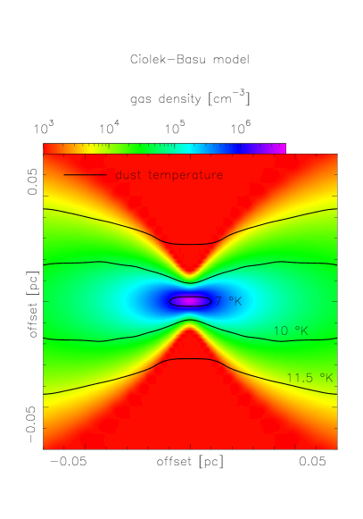
Figure 6: Dust density and temperature variation in the model of CB at time $t_{3}$ (2.66 Myr with central density $4.4\times 10^{6}$ $\hbox{{\rm cm}}^{-3}$)seen in the plane perpendicular to the disk midplane. The density variation shown in color is that of a flared disk. The temperature variation is given by the contours.

Another view of the temperature variation is presented in Fig. 6 which shows a cut perpendicular to the disk midplane. One sees that close to the midplane, the attenuation of the external radiation field is large and the temperature remains relatively low while in the perpendicular direction, it rises more rapidly. The temperature gradient is larger along the minor axis if one examines this model edge on. In practise, one must take into account effects due to finite inclination as well as the contributions from foreground and background layers.

5 Comparison of Models with Data

In this section, we present calculations of the mm–submm emission predicted by the models discussed above. We compute the expected intensity distributions and compare with observations of L1544. We consider first the spherically symmetric cases.

5.1 Intensity Distribution for spherically symmetric models

Figure 7: Intensity as a function of projected radius for the SIS and BES models discussed in section 2 and shown in Fig. 4. The top panel shows results at a wavelength of 1.3 mm, the center panel at a wavelength of 850 $\mu\hbox{m}$ and the bottom panel at a wavelength of 450 $\mu\hbox{m}$. We show results for the Bonnor–Ebert sphere (dashed) and SIS models (dotted line) with the Black radiation field and OH opacities. For comparison, we also show the expected distributions for a SIS model at a dust temperature of 12 K (solid).

Using the dust temperature distribution discussed earlier, we have computed the expected intensity distributions at three wavelengths for which observational data are available in the literature. These results have been obtained simply integrating the transport equation (with our calculated temperature distribution) across our model core. We have convolved the resultant intensity distribution with a “gaussian beam” of 13, 15 and 8^′′(at 140 pc) for 1.3 mm, 850, and 450 $\mu\hbox{m}$, respectively. We present in Fig. 7 results using the Black (1994) radiation field and compare the expected intensity profile at wavelengths mentioned above from the BES and SIS models.

One sees that at all wavelengths but especially at 450 $\mu\hbox{m}$, the profile is much flatter using our calculated temperature distribution than in the isothermal case. This just reflects the fact that the cold core nucleus predicted by our calculations does not contribute substantially at the shorter wavelengths. Even at 1300 $\mu\hbox{m}$, the contrast between the intensity at offset $10^{-3}$ pc (200 AU) and 0.1 pc is 26 in the isothermal case and 9 using our computed temperature gradient. Thus we conclude (in agreement with ERSM) that conclusions about the density structure based upon the intensity distribution of the dust continuum emission must take temperature gradients into account.

Another clear result from Fig. 7 is that the predicted intensity distributions for the BES and SIS models are essentially identical. The low temperature of the central nucleus causes the observed intensity profile to be insensitive to the density distribution inside 0.01 pc (2000 AU). This means that one should be very cautious about claims for a flat central density distribution based upon maps of millimeter dust emission. On the other hand, derivations of the density profile based upon either NIR reddening (Alves et al. 2001) or mid-IR extinction (Bacmann et al. 2000) are insensitive to dust temperature and hence are to be preferred for such purposes.

5.2 Intensity Distribution for the CB model

Figure 8: Intensity distribution (full lines) for wavelengths of 1.3 mm (top), 850 $\mu\hbox{m}$ (center), and 450 $\mu\hbox{m}$ (bottom) predicted by the CB model along the major axis (left hand panels) of L1544 and along the minor axis (right hand panels) assuming the density distribution at time $t_{3}$ (2.66 Myr) with central density $4.4\times 10^{6}$ $\hbox{{\rm cm}}^{-3}$ . In the panels for 850 $\mu\hbox{m}$ we also show profiles computed for the CB model at time $t_{4}$ (dash–dot, 2.68 Myr) and $t_{2}$ (dots, 2.60 Myr) (see caption for Fig.  5). An inclination of $16^{\circ}$ to the plane of the sky has been assumed. For comparison, we show also observed cuts along the major and minor axes of L1544 taken from Ward-Thompson et al. (1999) (1.3 mm data) and Shirley et al. (2000) (850$\mu\hbox{m}$ and 450 $\mu\hbox{m}$ data). The model intensity distribution has been convolved with gaussian beams with an HPBW of 13, 15 and 8 arc seconds for 1.3 mm, 850 $\mu\hbox{m}$ and 450$\mu\hbox{m}$, respectively, i.e. the same observational beam as the data.

The spherically symmetric models discussed above clearly do not apply to cores such as L1544 which has an extremely elongated intensity distribution when mapped at millimeter wavelengths (as well as an elongated appearance when observed in absorption at 7 $\mu\hbox{m}$ , Bacmann et al. 2000). We therefore now consider the expected intensity distributions for the models of CB shown in Fig. 5. One should note that these were originally constructed to fit the observed millimeter continuum intensity distribution for L1544 assuming isothermal dust. We now consider the consequences of the more realistic temperature distribution discussed above and compare with the available observations. We have again here used dust opacities from OH (thin ice, col. 5) and the external radiation field of Black (1994).

In Fig. 8, we show the resulting intensity distributions for the epoch $t_{3}$ of CB (central density $4.4\times 10^{6}$ $\hbox{{\rm cm}}^{-3}$). We have assumed an inclination of $16^{\circ}$ with respect to the plane of the sky as suggested by CB and compare with cuts along the major and minor axes from the work of Ward-Thompson et al. (1999) and Shirley et al. (2000). We conclude that despite departures from isothermality, the agreement between model and observed intensity distribution is reasonable at all three frequencies for time $t_{3}$. It certainly gives a better fit than the profile for time $t_{2}$ although it would be difficult to distinguish between $t_{3}$ (2.66 Myr) and $t_{4}$ (2.68 Myr) on this basis. Thus we confirm the result of CB that this stage in the development of their model fits the observed intensity distribution. We note nonetheless that in all cuts along the major axis, the fall off in observed intensity at positive offsets is more rapid than in the models.

Figure 9: Observed spectral energy distribution for L1544 compared with model predictions (solid lines) for the flux in a 40^′′ aperture as a function of wavelength. The model results are for the flux (Jy) in an aperture of 40^′′ HPBW towards the peak of the L1544 dust emission. Observational data (error bars) are from Shirley et al. (2000) and Ward–Thompson et al. (1999). The model data are for 3 different inclinations of a CB disk (time $t_{3}$) to the plane of the sky. The dashed line shows for comparison the expected SED for an isothermal CB disk inclined at 37^∘.

Another characteristic that a model should fit is the observed spectral energy distribution or SED. A complication here is that observations typically resolve pre–protostellar cores and that the SED thus depends sensitively on the assumed aperture. In Fig. 9, we present the expected spectrum for L1544 compared with observations from Shirley et al. (2000) for an assumed 40^′′ aperture (a compromise value). One sees that edge–on disks of this type are considerably stronger and easier to observe than face–on disks. This is because (even with a 40 ^′′beam at a distance of 140 pc) we resolve the source and as at these wavelengths, the model is optically thin, the flux is greater for the edge–on case where the column density is larger. We show for comparison the SED for the same model density distribution assumed to be isothermal and with an inclination of 37^∘. The isothermal model is slightly “hotter” than the model with computed temperature distribution and has a somewhat steeper long wavelength spectrum.

We get a reasonable agreement with the observed SED for an inclination of $37^{\circ}$ though this result reflects the assumed dust opacity and should be treated with caution. There is still considerable uncertainty concerning the nature of the ice mantles on the dust grains at the heart of pre–protostellar cores like L1544. We conclude nevertheless that the non–isothermal CB model at time $t_{3}$ does indeed give a reasonable fit to the observed flux distribution. The effects of departures from isothermality on the SED are probably small in comparison to the observational difficulties (e.g. due to pointing errors) of obtaining matched apertures at different frequencies towards an extended source. This is both because the fluxes from a 40^′′ region are not very sensitive to the central density distribution (i.e. the central 2000 AU) and because the low temperature causes a high density nucleus (if present) to have much less weight. This is in particular true at 850 $\mu\hbox{m}$ and higher frequencies and from this point of view, 1.3 mm observations of high angular resolution are needed to probe the nucleus of such cores.

Figure 10: Ratio of half-power sizes along the major and minor axes computed for CB model $t_{3}$ as a function of inclination of the mid–plane relative to the line of sight (full line). The measured ratio for L1544 is shown for comparison (dashed horizontal line) with upper and lower limits. The dotted lines show the axis ratios expected for a geometrically thin disk ($\sin{i}$) and for a geometrically thick disk using eq. (1) from CB (upper dotted curve) with ratio of disk thickness to radius 0.27.

As seen above, if we interpret cores like L1544 in terms of the CB model, the inclination of the CB disk to the line of sight is a critical parameter. It is also important for the interpretation of Zeeman effect observations (Crutcher & Troland 2001). This suggests that, for a model like that of CB, it is useful to estimate the inclination based upon the ratio of major and minor axes in a tracer such as the millimeter continuum. This must be done using so far as possible the true intensity distribution of the model core. With this in mind, we have attempted to calibrate the measurement using CB’s model at time $t_{3}$ and show the results in Fig. 10. We compare the results from the numerical computations with the formula given by CB for a disk of finite thickness as well as the simple result for a thin disk. Our computed axis ratio behaves rather like a thin disk at moderate inclinations but is close to the expected result in the edge–on case. We obtain from the axis ratios a best fit for an inclination of $37^{\circ}$ consistent with the SED of Fig.  9 shown above. However, our data would certainly accomodate an inclination of 25^∘ and (as Fig. 8 demonstrates) we cannot exclude 16^∘.

6 Discussion and Conclusions

This study has shown that departures from isothermality in pre–protostellar cores, while not a dominant effect, should be taken into account when considering core structure at times just prior to the onset of collapse. This is of importance when attempting to deduce the density structure of such regions based on maps of dust emission. It also may be important when considering the stability of such cores. Above densities of $10^{5}$ $\hbox{{\rm cm}}^{-3}$ , one expects gas and dust temperatures to be coupled (see Goldsmith 2001, Krügel & Walmsley 1984). Thus at higher densities in the center of cores such as L1544, one can expect the gas temperature to follow the dust temperature. A decrease in dust temperature in the nucleus of such cores requires a steeper density gradient than in an isothermal model and may have some consequences for the behavior of the mass accretion rate with time.

We have confirmed the ERSM conclusion that it is essentially impossible to distinguish a highly peaked density distribution (such as an SIS) from one with a flattened center (such as BE spheres) based on the millimeter maps. This has of course no consequences for methods of determining the dust column density distribution based upon absorption or extinction measurements (e.g. Alves et al. 2001, Bacmann et al. 2000). These other approaches however have their own limitations. For example, using NIR colors one is in practise limited to background giants seen in both H and K which puts an upper limit on the possible extinctions which are probed. The MIR technique on the other hand has problems both because one needs to distinguish between foreground and background radiation fields and because one is forced to make assumptions about the uniformity of the background field. Both these effects make it difficult to provide incontrovertible evidence of extinctions of order or larger than 100 magnitudes if present. We believe therefore that one should still be very cautious about ruling out peaked density distributions (such as the SIS) on the basis of the available data.

Using for the first time a reliable dust temperature distribution, we have obtained reasonable agreement between our models based upon the CB density distribution at time $t_{3}$ corresponding to a central density of $4\times 10^{6}$ $\hbox{{\rm cm}}^{-3}$ and the available millimeter and sub-millimeter data for L1544. This is a strong argument in favor of the validity of the model of CB as far as L1544 is concerned. We favor however higher inclinations of L1544 to the line of sight than given by CB and can fit both the SED and the aspect ratio for an inclination of 37^∘. There is on the other hand a considerable margin of error in this estimate and we do not entirely exclude the value of $16^{\circ}$ preferred by CB.

We conclude in any case that it would be useful to fit other cores with similar models. There may be some possibility in this way of relating the observed structure to “age” though it remains to be seen how effective this is in practise. The high central column density is the best indicator of an age close to the pivotal situation where dynamical collapse can commence. Unfortunately, the lower temperature of the high density nucleus caused by the increased extinction makes this high central column difficult to discern.

It should be realised also that other models are likely to be capable of fitting observational constraints. Recent relevant theoretical studies include those of Safier, McKee, and Stahler (1997), Galli et al. (2001) , and Indebetouw and Zweibel(2000). We note that Galli et al. (2001) obtain an excellent fit to the observed intensity distribution at 1.3 mm of L1544 with their model of a slightly inclined “singular isothermal disk” or SID. This is a non–axisymmetric structure with field lines running approximately in the line of sight. It would be useful also to compute the temperature structure of such a model in analogous fashion to that used in this paper for the CB models.

We have not considered in detail in this study the effect of external radiation fields other than the “standard” fields of MMP and Black (1994). However, it is likely that the actual fields incident upon dense cores vary from core to core and still more between molecular cloud and molecular cloud. Such differences plausibly occur due to the presence in the vicinity of nearby OB stars. The Bacmann et al. (2000) study (see their table 1 and subtract the zodiacal contribution) suggests that there may be as much as an order of magnitude difference in the ISO LW2 (5-8.5 $\mu\hbox{m}$) background towards different cores. It in fact also suggests that we underestimate by a factor of order 3 the field (at 7 $\mu\hbox{m}$) incident on L1544 using the Black (1994) average field. We have examined IRAS maps of L1544 and averaged intensities in an annulus surrounding the core with inner radius 100^′′ and outer radius 300^′′ centred on the mm dust emission peak. We conclude that the field adjacent to the core is a factor 2.5-4 greater than the Black (1994) field at 12 and 25 $\mu\hbox{m}$ suggesting that we underestimate the MIR contribution to the incident field (section 3). This may cause our temperature estimate to be low (by a factor of roughly 1.2) at extinctions of 20-30 magnitudes (see Fig.  2).

We may also be under–estimating the FIR field. L1544 is quite clearly present on IRAS 100$\mu\hbox{m}$ maps though not present at shorther wavelengths. This suggests that the incident UV–optical radiation field (presumably also responsible for exciting the MIR) is converted into far IR radiation in a “PDR” layer surrounding the cold core. This presumably should be added to the average incident field which we have used in our computations. We thus may also be underestimating the FIR heating.

We expect temperatures in these cores to vary as $\chi^{1/5.6}$ where $\chi$  is the scaling factor for the external radiation field (see section 3) and thus we expect differences as large as 1.5 between different objects. We would expect for example the nucleus of a core like OphD on this basis to be roughly 1.5 times hotter than L1544 using the mid IR intensities of Bacmann et al. (2000). This will have some effect on parameters such as the accretion rate but probably not an important one since the region where gas and dust temperatures are coupled is very limited. On the other hand, phenomena such as depletion of molecular species on grain surfaces are extremely sensitive to grain temperature and these are likely to have different characteristics depending on the precise grain temperature. This may explain why some of the chemical characteristics of cores in Ophiuchus and Taurus differ (long chain carbon species for example are much less prevalent in Ophiuchus) and may have consequences for the ionization degree at high densities.

One of the most useful products of this study is the analytic estimate which we have made of the temperature at the center of a spherically symmetric core. We have shown that the formula which we have derived gives in many cases a reasonable fit to the radial dependence of dust temperature and we believe it can be used as a useful first approximation to the gas temperature at densities above $10^{5}$ $\hbox{{\rm cm}}^{-3}$. Future studies can then perhaps consider the hydrostatic equilibrium of “Bonnor–Ebert spheres” for a more reasonable temperature distribution.

A brief summary of the results presented here as well as a more general discussion of the physical properties of pre–protostellar cores is given by Walmsley et al. (2001).

Appendix A The homogeneous spherical cloud

Consider a spherical, homogeneous cloud of radius $R$, exposed to an interstellar radiation field of mean intensity $J^{\rm is}_{\nu}$. Let $P$ be an internal point at a distance $r$ from the center $O$, and define a coordinate system centered in the center of the sphere with the $z$ axis along $OP$. Let $\theta$ be the angle between the $z$ axis and a generic direction in space originating from $P$. Considering only absorption by dust, the mean intensity in $P$ is

$$J_{\nu}(r)=\frac{J^{\rm is}_{\nu}}{4\pi}\int_{0}^{\pi}e^{-\tau_{\nu}(r,\theta)}2\pi\sin\theta\;d\theta,$$ (27)

where $\tau_{\nu}(r,\theta)$ is the optical depth of the cloud at frequency $\nu$ along a path from the point $P$ to the edge of the cloud in the direction $\theta$. Since the cloud is homogeneous, $\tau_{\nu}(r,\theta)$ is proportional to the distance from $P$ to the surface of the cloud,

$$\tau_{\nu}(x,\theta)=\tau_{\nu c}(\sqrt{1-x^{2}\sin^{2}\theta}-x\cos\theta),$$ (28)

where $\tau_{\nu c}$ is the optical depth at frequency $\nu$ to the center of cloud, and we have set $x\equiv r/R$. With the substitution $\eta\equiv\sqrt{1-x^{2}\sin^{2}\theta}-x\cos\theta$, eq. (27) becomes

$$J_{\nu}(x)=\frac{J^{\rm is}_{\nu}}{4x}\left[(1-x^{2})\int_{1-x}^{1+x}\frac{e^{-\tau_{\nu c}\eta}}{\eta^{2}}d\eta+\int_{1-x}^{1+x}e^{-\tau_{\nu c}\eta}d\eta\right].$$ (29)

Defining the auxiliary variables $x_{\pm}\equiv\tau_{\nu c}(1\pm x)$, the integral can be expressed in terms of exponential-integral functions,

$$J_{\nu}(x)=\frac{J^{\rm is}_{\nu}}{2(x_{+}-x_{-})}\times$$ (30)

$$\left[x_{+}E_{2}(x_{-})-x_{-}E_{2}(x_{+})+x_{-}E_{0}(x_{-})-x_{+}E_{0}(x_{+})\right],$$

where $E_{0}(x)=e^{-x}/x$. The values of $J_{\nu}(x)$ at the center and at the edge of the cloud are, respectively

$$J_{\nu}(0)=J^{\rm is}_{\nu}e^{-\tau_{\nu c}},$$ (31)

and

$$J_{\nu}(1)=\frac{J^{\rm is}_{\nu}}{4\tau_{\nu c}}(1+2\tau_{\nu c}-e^{-2\tau_{\nu c}}).$$ (32)

The value of $J_{\nu}$ at the edge of the cloud varies between $\frac{1}{2}J^{\rm is}_{\nu}$ for $\tau_{\nu c}\rightarrow\infty$ and $J^{\rm is}_{\nu}$ for $\tau_{\nu c}\rightarrow 0$.

Appendix B Parameters for the interstellar field and the opacity

We have (for the purpose of deriving the analytic formulae given in section 3.2) made approximate fits to the interstellar radiation field given by Black (1994) as well as to the grain opacities of Ossenkopf & Henning (1994). We approximate the radiation field by a sum of modified Planck functions given by eq. (6) and the opacity by piecewise power laws as follows.

For each black body (or modified) component of the interstellar radiation field, we give in Table  1 the values of the parameters $\lambda_{p}$, $p$, $W_{i}$, $T_{i}$ discussed in section 3.2.

The opacity parameters $\alpha$ and $Q_{\nu}$ for the different frequency ranges are also given in Table  2. These are based on the fact that one gets a rough fit (20 percent) to the Ossenkopf & Henning (1994) opacity results with a piecewise power law fit having an index 1.4 below 10 $\mu\hbox{m}$, 1.6 between 10 $\mu\hbox{m}$ and 400 $\mu\hbox{m}$, and 2 longward of 400 $\mu\hbox{m}$ (opacity proportional to $\nu^{\alpha}$). The parameters for dust emission ($Q_{e}$ and $\alpha_{e}$) used in the analytic formulation are appropriate for dust grains at roughly 10 K and we therefore use the values given for the wavelength range 10–400 $\mu\hbox{m}$ in Table  2.

Table 1: Parameters for the interstellar field

range	$\lambda_{p}$	$p$	$W_{i}$	$T_{i}$
				($K$)
V–NIR	0.4 $\mu\hbox{m}$	0	$1\times 10^{-14}$	7500
	0.75 $\mu\hbox{m}$	”	$1\times 10^{-13}$	4000
	1 $\mu\hbox{m}$	”	$4\times 10^{-13}$	3000
MIR	100 $\mu\hbox{m}$	$-1.8$	$5\times 10^{-7}$
FIR	140 $\mu\hbox{m}$	1.65	$2\times 10^{-4}$	23.3
CBR	1.06 mm	0	1	2.728

Table 2: Parameters for the opacity

wavelength range	$\lambda_{\rm a}$	$Q_{\nu}$ at $\lambda_{\rm a}$	$\alpha$
		(cm2 H${}_{2}^{-1}$)
0.1–10 $\mu\hbox{m}$	1 $\mu\hbox{m}$	$3.9\times 10^{-22}$	1.4
10–400 $\mu\hbox{m}$	140 $\mu\hbox{m}$	$1.5\times 10^{-24}$	1.6
400 $\mu\hbox{m}$–10 mm	1.06 mm	$3.3\times 10^{-26}$	2.0

References

- (1) Alves, J.F., Lada C.J., Lada E.A. 2001, Nature 409,159
- (2) André, P., Ward–Thompson, D., Barsony, M. 2000, in Protostars and Planets IV, edited by V. Mannings, A. P. Boss, S. S. Russell, (Univ. of Arizona press: Tucson), p. 59
- (3) Bacmann, A., André, P., Puget, J.-L., Abergel, A., Bontemps, S., Ward–Thompson, D. 2000, A&A, 361, 555
- (4) Black, J.H. 1994, in The First Symposium on the Infrared Cirrus and Diffuse Interstellar Clouds, ASP Conf. Series 58, edited R. M. Cutri and W. B. Latter, p. 355
- (5) Basu, S. 2000, ApJ, 540, L103
- (6) Bonnor, W.B. 1956, MNRAS, 116, 351
- (7) Boulanger, F., Cox, P., Jones, A.P. 2000, in Infrared Space Astronomy: today and tomorrow, edited by F. Casoli, J. Lequeux, F. David (Springer-Verlag), p. 251
- (8) Chandrasekhar, S. 1939, An Introduction to the Study of Stellar Structure, Univ. of Chicago Press
- (9) Ciolek, G.E., Basu, S. 2000, ApJ, 529, 925
- (10) Ciolek, G.E., Basu, S. 2000, in From Darkness to Light, edited by T. Montmerle and P. André, ASP Conference Series (in press)
- (11) Crutcher, R.M., Troland T.H. 2000, ApJ, 537, L139
- (12) Ebert, R. 1955, Z. Astrophys., 37, 217
- (13) Evans, N.J.II, Rawlings, J.M.C., Shirley, Y.L., Mundy, L.G. 2001, ApJ (in press) (ERSM)
- (14) Flannery, B. P., Roberge, W., Rybicki, G. R. 1980, ApJ, 236, 598
- (15) Galli, D., Shu, F. H., Laughlin, G., Lizano, S. 2001, ApJ, 551, 367
- (16) Goldsmith, P.F., 2001, ApJ (in press)
- (17) Indebetouw, R., Zweibel, E.G. 2000, ApJ, 532, 361
- (18) Kramer, C., Alves, J., Lada, C., Lada, E., Sievers A., Ungerechts, H., Walmsley, C.M. 1997, A&A , 329, L33
- (19) Krügel, E., Walmsley, C.M. 1984, A&A, 130, 5
- (20) Leung, C.M. 1975, ApJ, 199, 340
- (21) Mathis, J.S., Mezger, P., Panagia, N. 1983, A&A, 128, 212 (MMP)
- (22) Mathis, J.S. 1990, Ann. Rev. Astron. Astrophys. 28, 37
- (23) McKee, C.F. 1999, in The Origin of Stars and Planetary Systems, edited C.J.Lada and N.Kylafis, NATO Science Series C 540, publ. Kluwer Academic, p. 29
- (24) Ossenkopf, V., Henning, T. 1994, A&A, 291, 943
- (25) Safier, P.N., McKee, C.F., Stahler, S. 1997, ApJ, 485, 660
- (26) Shirley, Y.L., Evans, N.J.II, Rawlings J.M.C., Gregersen, E.M. 2000, ApJS, 131, 249
- (27) Shu, F. H. 1977, ApJ, 214, 488
- (28) Shu, F.H., Adams, F.C., Lizano, S. 1987, ARAA, 25, 31
- (29) Spitzer, L. 1978, Physical Processes in the Interstellar Medium (Wiley)
- (30) Tafalla, M., Mardones, D., Myers, P. C., Caselli, P., Bachiller, R., Benson, P.J. 1998, ApJ, 504, 900
- (31) Walmsley, C.M., Caselli, P., Zucconi, A., Galli, D. 2001, in Origins of stars and planets: The VLT View, edited J. Alves, M. McCaughrean, publ. Springer Verlag.
- (32) Ward–Thompson, D., Motte, F., André, P. 1999, MNRAS, 268, 276
- (33) Ward–Thompson, D., Kirk, J.M., Crutcher, R.M., Greaves, J.S., Holland, W.S., André, P. 2000, ApJ, 537, L135
- (34) Williams, J.P., Myers, P.C., Wilner, D.J., Di Francesco, J. 1999, ApJ, 513, L61
- (35) Wright, E.L. et al. 1991, ApJ, 381, 200