Strong Shocks and Supersonic Winds in Inhomogeneous Media
Abstract
Many astrophysical flows occur in inhomogeneous media. The broad-line regions (BLR) of active galactic nuclei (AGNs) are one of the important examples where emission-line clouds interact with the outflow.
We present results of a numerical study of the interaction of a steady, planar shock / supersonic postshock flow with a system of embedded cylindrical clouds in a two-dimensional geometry. Detailed analysis shows that the interaction of embedded inhomogeneities with the shock / postshock wind depends primarily on the thickness of the cloud layer and the arrangement of the clouds in the layer, as opposed to the total cloud mass and the total number of individual clouds. This allows us to define two classes of cloud distributions: thin and thick layers. We define the critical cloud separation along the direction of the flow and perpendicular to it. This definition allows us to distinguish between the interacting and noninteracting regimes of cloud evolution. Finally we discuss mass-loading in such systems.
Department of Physics and Astronomy,
University of Rochester, Rochester, NY 14627-0171
1. INTRODUCTION
Mass flows are important in many astrophysical systems from stars to the most distant active galaxies. Virtually all mass flow studies focus on homogeneous media. However, the typical astrophysical medium is inhomogeneous with the inhomogeneities (clumps) arising due to initial fluctuations of mass distribution, the action of instabilities, variations in the flow source, etc. The presence of inhomogeneities can introduce not only quantitative but also qualitative changes to the overall dynamics of the flow.
Active galactic nuclei represent one astrophysical site where a shock / wind interaction with a system of inhomogeneities may take place. Practically all current models of AGNs agree that the emission-line clouds in BLRs are essential for explaining the observed properties of AGNs (Urry & Padovani 1995; Elvis 2000). However, despite the fact that the nature of BELR clouds is an open question, any self-consistent model of the AGNs should properly account for properties of BELR cloud interaction with mass outflow. In particular, such self-consistency is important in the context of cloud survival time and cloud displacement prior to destruction. Even when clouds are magnetically confined and stabilized against evaporation (Rees 1987), disruptive action of outflows may prevent cloud survival over the dynamically significant AGN timescales.
(Klein, McKee, Colella 1994) (hereafter KMC) addressed the problem of shock-cloud interaction, providing a detailed description of the dynamics of a single, dense, unmagnetized cloud interacting with a strong, steady, planar shock. That work gives an excellent introduction to the subject, in particular the description of the astrophysical significance of the problem of a shock wave interacting with a dense cloud (see also (Gregori et al. 2000)). In this work we investigate the general properties of strong shock / supersonic wind interaction with a system of embedded clouds and determine the key quantities governing the evolution of such systems.
2. RESULTS
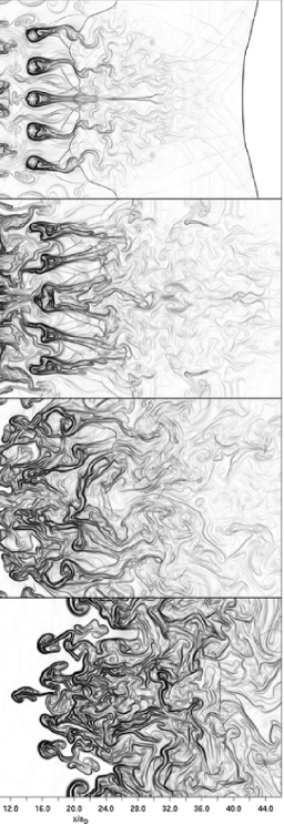
We have numerically investigated the interaction of a strong, planar shock wave with a system of dense inhomogeneities, embedded in a more tenuous and cold ambient medium. Our code is the AMRCLAW package, which implements an adaptive mesh refinement algorithm for the equations of gas dynamics (Berger & Oliger 1984; Berger & Jameson 1985; Berger & Colella 1989; Berger & LeVeque 1998) in two dimensions. We have assumed constant conditions in the global postshock flow constraining the maximum size of the clouds only by the condition of the shock front planarity. Our results are applicable to strong global shocks with Mach numbers . The range of the applicable cloud - unshocked ambient medium density contrast values is . Figure 1 shows a case of a strong shock and a supersonic post-shock flow interacting with an inhomogeneous system of fourteen identical clouds in regular distribution.
Cloud evolution due to the interaction with the global shock and the postshock flow has four major phases, namely the initial compression phase, the re-expansion phase, the destruction phase, and finally the mixing phase. Each image in Figure 1 roughly illustrates each of those phases.
The timescale we use to define time intervals in our numerical experiments is the time it takes for the incident shock wave to sweep across an individual cloud. This is called the shock-crossing time, , where is the maximum cloud radius in the distribution.
We define the cloud destruction time as the time when the largest cloud fragment contains less than 50 of the initial cloud mass. Typically, in our simulations .
A simple model for the cloud acceleration during the first three phases, i.e. prior to its destruction, can be developed. We find the cloud velocity
| (1) |
Here, is the unperturbed postshock flow velocity. For the cases of infinitely strong shocks, i.e. , the above coefficients have the values
| (2) |
Equation (1) shows that the maximum cloud velocity is not more than of the global shock velocity and not more than of the postshock flow velocity.
Cloud displacement prior to its destruction can be described as
| (3) |
In the limiting case the values of the coefficients and are defined in (2) and
We find the maximum cloud displacement prior to its destruction, , is
| (4) |
The results of our model are in excellent agreement with the numerical experiments. The difference in the values of cloud velocity and displacement between analytical and numerical results is .
The principal conclusion of the present work is that the set of all possible cloud distributions can be subdivided into two large subsets , thin-layer systems, and , thick-layer systems, defined as
| (5) |
where is the maximum cloud separation in the system along the direction of the flow, or the cloud layer thickness.
Distributions from each subset exhibit striking similarity in behaviour (e.g. Figure 2). The systems containing from one to five clouds, arranged in a single layer, exhibit exactly the same rate of momentum transfer from the global flow to the clouds. The two fourteen cloud runs and have different cloud distributions, different total cloud mass, different cloud sizes. Nevertheless, the rate of the kinetic energy fraction increase during compression and re-expansion is different from the single layer cases but is still the same for both fourteen cloud runs. Other global properties exhibit the same behaviour. We conclude that the evolution of a system of shocked clouds depends primarily on the total thickness of the cloud layer and the cloud distribution in it, as opposed to the total number of clouds or the total cloud mass present in the system.
The key parameters determining the type of evolution, are the cloud destruction length , defined above in (3), and the critical cloud separation transverse to the flow . The latter is defined by the condition that the time for adjacent clouds to expand laterally and merge into a single coherent structure is equal to the cloud destruction time . It can be described by the expression
| (6) |
We should be able to determine, either from observations or from theoretical analysis, the thickness of the cloud layer . This determines the class of the given cloud distribution, or . For distributions from the set with average cloud separation evolution of the clouds during the compression, re-expansion, and destruction phases will proceed in the noninteracting regime and the formalism for a single cloud interaction with a shock wave (e.g. KMC) can be used to describe the system. On the other hand, if the cloud separation is less than critical, the clouds in the layer will merge into a single structure before their destruction is completed, and though the compression phase still can be considered independently for each cloud, evolution during the re-expansion and destruction phases proceeds in the interacting regime.
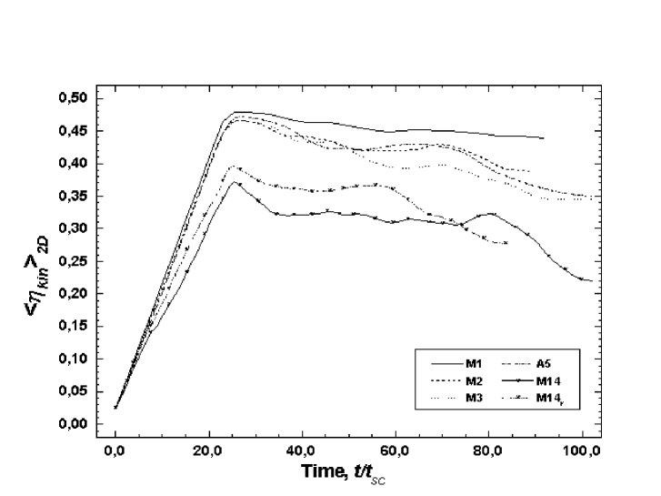
, , , - systems with 1, 2, 3, 5 identical clouds correspondingly, arranged in a single row with constant cloud center separation of ; - system with 14 identical clouds with cloud center separation in a row equal to , separation between rows equal to ; - system with 14 clouds of random size and placed in random positions.
When the distribution belongs to the subset it is necessary to determine the average cloud separation projected onto the direction of the flow and compare it against : if evolution of the system can be roughly approximated as of a set of distributions from the subset and the above “thin-layer case” analysis applies. If, on the other hand, (especially if ) the system evolution is dominated by cloud interactions and a thin layer formalism is inapplicable.
Finally we consider mass-loading. Here our principal conclusion is that mass-loading is not significant in the cases of strong shocks and supersonic winds interacting with inhomogeneities whose density contrast is in the range . In part this is due to short survival times of clouds as well as the very low mass loss rates of the clouds even during the times prior to their destruction. Therefore, mass-loading in such systems is not likely to have any appreciable effect on the overall dynamics of the global flow.
The major limitation of our current work is the purely hydrodynamic nature of our analysis that does not include any consideration of the magnetic fields. As was discussed by KMC, cold dense inhomogeneities (clouds) embedded in more tenuous hotter medium are inherently unstable against the dissipative action of diffusion and thermal conduction. Although weak magnetic fields, that are dynamically insignificant up to the moment of cloud destruction, can inhibit thermal conduction and diffusion and, therefore, stabilize the system of clouds, those magnetic fields may become dynamically important due to turbulent amplification during the mixing phase (see (Gregori et al. 2000) for a three-dimensional study of the wind interaction with a single magnetized cloud). We intend to provide a fully magnetohydrodynamic description of the interaction of a strong shock with a system of clouds in future work.
Acknowledgments.
This work was supported in part by the NSF AST-0978765, NASA NAG5-8428,
and DOE DE-FG02-00ER54600 grants.
The most recent results and animations of the numerical experiments,
described above and not mentioned in the current paper, can be found
at
www.pas.rochester.eduwma.
References
Berger, M.J., Colella, P. 1989, J. Comp. Phys., 82, 64
Berger, M.J., Jameson, A. 1985, AIAA J., 23, 561
Berger, M.J., LeVeque, R.J. 1998, SIAM J. Numer. Anal., 35, 2298
Berger, M.J., Oliger, J. 1984, J. Comp. Phys., 53, 484
Gregori, G., Miniati, F., Ryu, D., Jones, T.W. 2000, ApJ, 543, 775
Elvis, M. 2000, ApJ, 545, 63
Klein, R.I., McKee, C.F., Colella, P. 1994, ApJ, 420, 213
Pietrini, P., Torricelli-Ciamponi, G. 2000, A&A, 363, 455
Rees, M.J. 1987, MNRAS, 228, 47
Urry, C.M., Padovani, P. 1995, PASP, 107, 803