The 3D-structure of the LISM

Abstract

We review what is currently known about the structure of interstellar material in the solar neighborhood, emphasizing how observations from the Hubble Space Telescope (HST) have improved our understanding of how interstellar gas is distributed near the Sun. The nearby ISM is not uniform but shows variations in both temperature and metal abundances on distance scales of just a few parsecs. The observations also show that nearby gas does not have a single uniform velocity vector. Instead, different components are often seen in different directions for even very short lines of sight. However, interpretation of these components remains difficult. It is uncertain whether the components represent physically distinct clouds or perhaps are just symptomatic of velocity gradients within the cloud. Finally, since it is the local interstellar medium’s interaction with the solar wind that is the primary application of ISM studies considered in these proceedings, we also review how the same HST data used to study the local ISM structure has also been used to study both the heliospheric interaction with the solar wind and also “astrospheric” interactions with the winds of other stars.

1 INTRODUCTION

The Sun resides within a region of space called the Local Bubble, which extends about 100 pc in most directions [1]. The existence of the Local Bubble was first apparent on the basis of just how little ISM material was generally observed within roughly 100 pc. Later, the hot material within the Bubble was detected directly from X-ray observations. Most locations within the the Local Bubble are very hot ($T\sim 10^{6}$ K) and rarified ($n_{e}\sim 10^{-3}$ cm^-3). The ISM is therefore completely ionized.

However, the local interstellar medium (LISM) material immediately around the Sun appears to be of a different character. Observations of solar Ly$\alpha$ emission scattering off interstellar H I gas flowing into the heliosphere revealed that the LISM is at least partially neutral. Furthermore, it is cooler ($T\sim 10^{4}$ K) and denser ($n_{e}\sim 10^{-1}$ cm^-3) than the hot plasma filling most of the Local Bubble [2, 3]. Further studies, both of the solar backscatter variety and of interstellar absorption lines, have further refined our understanding of the LISM, which we consider for our purposes here to be the warm, partially ionized ISM within roughly 10–20 pc of the Sun. We now discuss how recent observations, especially from the Hubble Space Telescope (HST), have continued to both clarify and complicate our understanding of the LISM.

2 THE ANALYSIS OF ABSORPTION LINE DATA

2.1 The H I and D I Ly$\alpha$ Lines

Since its launch in 1990, HST has been a very useful source of information about the LISM, in particular the high resolution UV spectrometers carried by the satellite, first the Goddard High Resolution Spectrograph (GHRS) followed by the Space Telescope Imaging Spectrograph (STIS) that replaced GHRS in 1997. Earlier UV-based satellites, particularly the International Ultraviolet Explorer (IUE) and Copernicus missions provided the first extensive absorption line studies of very nearby ISM material [4, 5, 6, 7, 8, 9]. However, GHRS and STIS are the first UV instruments to offer spectral resolution sufficient to fully resolve narrow LISM absorption lines, enabling the separation of closely spaced velocity components and allowing more accurate measurements of the absorption features.

Because there are very few hot stars within 10–20 pc of the Sun, most absorption line studies of the LISM rely on observations of cool stars. The disadvantage of working with cool star UV spectra in an ISM analysis is that cool stars do not have strong continua in the far-UV (FUV) below 2000 Å. This limits the number of detectable lines, since one can only detect an ISM line if it happens to lie on top of a stellar emission line. The most important LISM absorption line accessible to HST is the H I Ly$\alpha$ line. Analysis of H I absorption in this spectral feature provides column density measurements of the most abundant atom in the LISM, and the universe in general, neutral hydrogen. Fortunately, cool star chromospheres provide copious amounts of H I Ly$\alpha$ emission to provide a background against which the ISM absorption can be seen.

In Figure 1, we show an example of the type of HST cool star Ly$\alpha$ spectra typically used to study H I in the LISM [10]. The observations are for the two primary members of the closest star system to the Sun, the $\alpha$ Cen system, which is only 1.3 pc away and also contains a third distant member, Proxima Cen. The prevalence of H I means that even for the shortest lines of sight the LISM H I absorption is always seen to be very broad and saturated.

Figure 1: HST/GHRS spectra of the Ly$\alpha$ lines of $\alpha$ Cen A and B, showing broad absorption from interstellar H I and narrow absorption from D I [10].

Measurements of saturated lines are unfortunately not as precise as measurements of weaker, unsaturated lines. However, the opacity of H I Ly$\alpha$ is so high that at typical LISM column densities of $\log{\rm N(H~{}I)}\approx 18.0$ (in cm^-2) the line is starting to leave the flat part of the curve of growth. In other words, the Lorentzian wings of the opacity profile are starting to come into play, subtly altering the shape of the absorption profile and allowing the H I measurement to be somewhat more accurate than a measurement of a line fully in the flat part of the curve of growth. Furthermore, the H I analysis can also benefit if it is combined with the analysis of the nearby deuterium (D I) Ly$\alpha$ line, which is the narrow, unsaturated line visible just blueward of the H I line in Figure 1.

There are three free parameters in any absorption line fit: the centroid velocity, $v$, the Doppler parameter, $b$, and the column density, $N$. The Doppler parameter is connected with the temperature ($T$) and turbulent (i.e., nonthermal) velocity ($\xi$) of the absorbing gas by the equation

$$b^{2}=0.0165T/A+\xi^{2},$$ (1)

where $A$ is the atomic weight of the atom or ion responsible for the absorption, and $b$ and $\xi$ both have units of km s^-1. The centroid is generally easy enough to measure for any absorption line since it is independent of the other parameters, but for saturated lines the Doppler parameter and column density are correlated. This means that, relative to a “best fit,” there may be fits of nearly equal quality with lower $b$ and higher $N$, or higher $b$ and lower $N$. Therein lies the difficulty with accurately analyzing H I Ly$\alpha$ by itself.

However, the D I line, which is generally optically thin in the LISM, does not have this problem. For an optically thin line, $b$ and $N$ are essentially independent, with $b$ being associated with the width of the absorption line and $N$ with its depth. In section 2.2, we will describe how comparing the $b$ values of lightweight atoms (with low $A$) with those of heavier atoms can yield a unique measurement of $T$ and $\xi$ using equation (1). Such analyses clearly show that in the LISM, H I and D I are dominated by thermal broadening. This means that if the H I and D I Ly$\alpha$ lines are fitted simultaneously, one can add the constraint that $b({\rm D~{}I})=b({\rm H~{}I})/\sqrt{2}$. This additional constraint removes some of the dependence of $b({\rm H~{}I})$ on $N({\rm H~{}I})$, allowing both quantities to be measured more accurately. In such H I and D I fits it is also typically assumed that the centroid velocities of H I and D I are the same, which is an important constraint if the H I absorption is affected by a source of absorption not observed in D I. This is the case when heliospheric or “astrospheric” material contributes to the H I absorption (see section 4).

The D I line is, of course, of interest in its own right, not just as an aid to measuring H I. The deuterium-to-hydrogen ratio (D/H) in the universe is a very important quantity both for cosmology and Galactic chemical evolution studies [11, 12, 13, 14]. Thus, many of the LISM analyses of Ly$\alpha$ lines have focused on measuring D/H, including many of the first analyses of HST data [4, 7, 9, 15, 16, 17, 18]. One important issue concerns how well mixed the Galactic ISM is and if there are large variations of D/H within the ISM. Measurements within what we are calling the LISM (i.e., within 10-20 pc) suggest ${\rm D/H}=(1.5\pm 0.1)\times 10^{-5}$ with little if any evidence for variation [19]. This uniformity of at least the very local ISM has allowed some Ly$\alpha$ studies of the LISM to constrain $N({\rm H~{}I})$ by assuming the above D/H ratio [20, 21, 22], which is a reasonable thing to do if the quality of the data is such that an accurate $N({\rm H~{}I})$ value cannot be derived without constraining it with $N({\rm D~{}I})$. Note, however, that there is evidence for D/H variations on distance scales of $\sim 100$ pc and larger [23, 24, 25], making this assumption questionable for longer lines of sight.

2.2 The Metal Lines

In order to obtain the most accurate analysis of the Ly$\alpha$ line it is necessary to know the number of interstellar components along the line of sight. Unfortunately, the large widths of both the H I and D I lines (due to their low $A$ values) means these lines are not very useful for looking for multiple ISM components along the line of sight, since closely spaced velocity components will be too highly blended within the H I and D I lines to be distinguishable. Thus, the most accurate LISM studies also require high resolution observations of narrow absorption lines of heavy atoms, in addition to the Ly$\alpha$ data.

The three most commonly observed metal lines that are useful for these purposes are the Mg II h & k lines with vacuum wavelengths of 2803.531 Å and 2796.352 Å, respectively, and the Fe II $\lambda$2600.173 line. Figure 2 shows the Fe II absorption observed towards $\alpha$ Cen, plotted on a heliocentric velocity scale [10]. The Fe II line was observed by HST/GHRS on two separate occasions so there are two spectra of the same line shown in the figure. An absorption line fit is also shown, where the dotted line is the fit before convolution with the instrumental profile and the thick solid line that fits the data is the fit after the instrumental broadening is taken into account. The difference between the two indicates the degree to which the HST/GHRS instrument is resolving the line. These fits require the stellar background flux be estimated (i.e., thin solid lines in Fig. 2), but this is a relatively easy thing to do for narrow lines like Fe II and Mg II. Polynomial fits to the continuum, excluding the LISM absorption, adequately estimate the stellar flux above the absorption.

Figure 2: Fits to the interstellar Fe II $\lambda$2600.2 absorption line observed towards $\alpha$ Cen A by HST/GHRS, once in 1992 and again in 1995. The dotted and thick solid lines are the fits before and after convolution with the instrumental profile, respectively [10].

Figure 2 shows that the LISM absorption towards $\alpha$ Cen is fitted nicely with only a single absorption component. Many lines of sight through the LISM have this desirable property, which simplifies the analysis of the absorption line data. However, many lines of sight also show multiple components, including many short lines of sight to very nearby stars. Figure 3 shows the Mg II h & k absorption lines observed towards 61 Cyg A, a star only 3.5 pc away [21]. Two LISM absorption components are required to fit these two lines. Other very nearby stars with LISM absorption features indicating more than one component include Sirius ($d=2.6$ pc) [26], Procyon ($d=3.5$ pc) [16], and Altair ($d=5.1$ pc) [27].

Figure 3: Two-component fits to the interstellar Mg II absorption lines seen towards 61 Cyg A, with the individual components shown as dotted lines and the combination of the two components shown as thick solid lines (after convolution with the instrumental profile). The shaded region was ignored in the fit due to contamination from a stellar absorption line [21].

The existence of these multiple velocity components means that the LISM is not characterized by a single velocity vector. However, in all the multiple-component cases mentioned above the components are not widely separated, and this is generally the case within the LISM. Thus, the different velocity vectors are not in widely disparate directions or with very different speeds. Instead, they are all presumably minor variations of basically the same vector. Whether the individual components represent different, physically distinct clouds is a complicated question that we will return to in section 3.3.

Besides their usefulness in establishing the velocity structure of LISM lines of sight, the metal lines are also useful in measuring the temperature ($T$) and nonthermal velocity ($\xi$) of the LISM. Figure 4 shows how this is done for the case of the $\alpha$ Cen line of sight [10]. Based on the measured Doppler parameters and equation (1), $\xi$ is plotted versus $T$ for Fe II, Mg II, and D I. Thanks to the different atomic weights of these elements, the curves have different slopes. The intersection of the curves indicates the $T$ and $\xi$ value for the line of sight. Values of $T=5400\pm 500$ K and $\xi=1.20\pm 0.25$ km s^-1 are suggested by Figure 4.

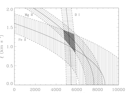
Figure 4: Nonthermal velocities ($\xi$) are plotted versus temperature, based on the Doppler parameters and their uncertainties measured from absorption lines of Fe II, Mg II, and D I observed towards $\alpha$ Cen. The shaded area where the three curves overlap indicates the actual temperature and $\xi$ value of the interstellar material [10].

3 THE PHYSICAL STRUCTURE OF THE LISM

3.1 The Local Interstellar Cloud

The cloud within the LISM in which the Sun resides is generally referred to as the Local Interstellar Cloud (LIC). The properties of the LIC have been studied in two fundamentally different ways. One method is by studying LISM absorption lines, as described in section 2. The other method relies on observations of interstellar gas within the heliosphere. Detection of solar Ly$\alpha$ emission scattered back toward Earth by interstellar H I flowing through the heliosphere provided the first evidence that the surrounding ISM was at least partially neutral [28], and Ly$\alpha$ backscatter within the heliosphere still remains a valuable source of information about the LIC and its interaction with the solar wind. The SWAN instrument on the SOHO satellite has provided the most recent observations of this sort [29, 30]. There are also direct in situ studies of interstellar atoms within the heliosphere that have been made by interplanetary spacecraft. Of particular note are the observations from the Ulysses satellite [31, 32].

Both measurements of ISM material flowing through the heliosphere and LISM absorption line studies have been used to estimate the direction and magnitude of the LIC vector [31, 32, 27, 30], and the resulting LIC vectors are in good agreement. The vector derived from the absorption lines has a magnitude of 25.7 km s^-1 directed towards Galactic coordinates $l=186.1^{\circ}$ and $b=-16.4^{\circ}$ [27, 33]. With this vector, LISM absorption from the LIC can be identified for any line of sight by its centroid velocity.

By measuring LIC column densities for many lines of sight in many different directions, a three dimensional model of the shape of the LIC can be constructed [34]. Figure 5 shows a map of the H I column density between the Sun and the edge of the cloud in Galactic coordinates. The locations of various lines of sight used in the construction of the model are indicated. Observations from the Extreme Ultraviolet Explorer (EUVE) and some optical Ca II measurements were used to supplement the HST data and fill in gaps left by the HST-observed lines of sight. The largest column density is about $2\times 10^{18}$ towards Galactic coordinates $l=157^{\circ}$ and $b=-25^{\circ}$. There is very little if any column in the direction of the Galactic Center ($l=0^{\circ}$), indicating we are very near the edge of the cloud in this direction. This would be the direction of the so-called G cloud, which will be discussed in section 3.2.

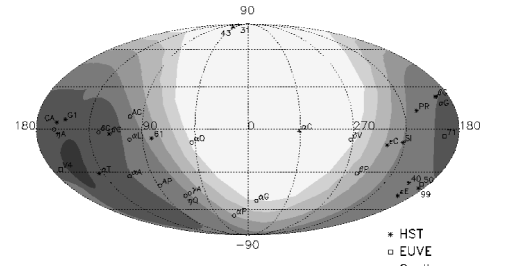
Figure 5: Map in Galactic coordinates of the H I column density from the Sun to the edge of the LIC, with the contour edges from darkest to lightest representing columns (in units of $10^{18}$ cm^-2) of 2.0, 1.0, 0.5, 0.25, 0.10, and 0.05. Positions of stars used in the creation of this 3D LIC model are also plotted, with the symbol indicating if the data was obtained by HST, EUVE, or by ground-based observations of Ca II [34].

The highest average H I densities seen towards the nearest stars are of order $n({\rm H~{}I})=0.1$ cm^-3, so we assume this is representative of the average density within the cloud. Estimates of $n({\rm H~{}I})$ from heliospheric observations suggest somewhat higher densities of $n({\rm H~{}I})\approx 0.2$ cm^-3 [35, 36], possibly suggesting the presence of density and/or hydrogen ionization state variations within the LIC. In any case, assuming $n({\rm H~{}I})=0.1$ cm^-3 as an average LIC density, the observed column densities in Figure 5 translate to a cloud about 5–7 pc across depending on the direction, with a volume of 93 pc³, and a total mass of about 0.32 M_⊙ [34].

Temperatures have been measured for the LIC for many lines of sight using the technique shown in Figure 4. These temperatures range from $T=6900\pm 380$ K towards Procyon [16] to $T=9700\pm 900$ K towards $\beta$ Cas [17], so it is possible that there is some variation within the LIC. The weighted mean and standard deviation of all the LIC measurements is $T=8000\pm 1000$ K [17, 18, 21]. Turbulent velocities are not as well determined but generally $\xi\leq 2$ km s^-1.

The most recent temperature determination from Ulysses observations of interstellar He I within the heliosphere, $T=5800\pm 700$ K [32], is lower than the absorption line measurements. This might be further evidence for a temperature gradient within the LIC and within the LISM in general. Because of the Sun’s location very near the edge of the LIC, most of the absorption line studies measuring LIC properties are in a generally anti-Galactic center direction ($90^{\circ}<l<270^{\circ}$), as shown in Figure 5. Lines of sight roughly towards the Galactic center sample G cloud material rather than LIC material (see section 3.2). The G cloud is cooler than the LIC so the Ulysses measurement and absorption line measurements of the G and LIC clouds together suggest a possible temperature gradient in the LISM, with lower temperatures towards the Galactic Center and higher temperatures in the opposite direction where most of the LIC resides.

The ionization state of the LIC is an issue that remains complicated both observationally and theoretically. Many attempts to measure the electron density ($n_{e}$) in the LIC have been based on the observed ionization states of magnesium or sodium, but these measurements tend to have large uncertainties since the ionization state dependence on $n_{e}$ is also highly temperature dependent [37, 38]. Furthermore, there is still some question as to whether the LIC is actually in ionization equilibrium at all [39], and if it is not then it will not be possible to estimate $n_{e}$ from the ionization state of any element. A final complication is that the ionization state of the LIC can be expected to be variable within the cloud, since the ionization state at a given location will depend on how shielded that location is from various photoionization sources by intervening LISM material [40, 41].

The best measurement of $n_{e}$ in the LIC comes from observations of C II lines towards Capella, which are shown in Figure 6 [42]. The C II $\lambda$1335 transition is from the ground state, which is where most C II ions in the LISM will reside. The C II $\lambda$1336 transition is from an excited state that is much less populated than the ground state, explaining why the $\lambda$1336 line is so much weaker than the $\lambda$1335 line. The excited state represented by the $\lambda$1336 line is populated by collisions with electrons, and so the column density ratio of the two C II lines will depend on the electron density in the LIC. The advantage of this method for measuring $n_{e}$ is that it is not temperature dependent and does not assume ionization equilibrium. However, since the $\lambda$1335 line is saturated, the ground state C II column density has large uncertainties and therefore so does the derived electron density: $n_{e}=0.11^{+0.12}_{-0.06}$ cm^-3 [42]. This value is roughly consistent with estimates of the proton density that have been made based on heliospheric observations [36].

Figure 6: HST/GHRS spectrum of the C II $\lambda\lambda$1335, 1336 emission lines of Capella. Interstellar C II absorption features are marked with vertical dotted lines [42].

The electron density in the LIC is comparable to the average LIC $n({\rm H~{}I})$ value quoted above. This means that hydrogen in the LIC is roughly half-ionized since hydrogen will be the dominant source of electrons in the LIC. This is too high of an ionization state to be explained by collisional ionization at a temperature of about 8000 K. It has therefore been generally assumed that the extreme UV background flux provided by surrounding hot stars and hot ISM photoionizes the LISM and determines its ionization state. Observations from EUVE suggest that the photoionizing flux from hot stars can indeed explain the half-ionized state of hydrogen [39].

However, EUVE has also found that helium is also roughly half-ionized in the LISM, which is much harder to explain due to its higher ionization potential [43, 44, 45]. The stellar EUV background flux cannot seem to explain the He ionization state, but while the stellar sources of ionizing photons are known well, the diffuse EUV background provided by the hot ISM in the local bubble and its interaction with neutral clouds is not well known, so the issue of whether the ionization state of the local cloud is entirely determined by photoionization is still open. An alternative theory is that the local cloud is not in ionization equilibrium at all, but was instead collisionally ionized a million years or so ago by a passing shock wave, perhaps from a nearby supernova, and still has not recombined to an equilibrium state [39].

3.2 The G Cloud

Figure 7 shows the outline of the LIC in the Galactic plane based on the model in Figure 5 described above [34]. The Sun is very near the edge of the cloud in the Galactic Center direction. The placement of the Sun at this location so near the edge is based on the discovery that when you look in this direction you do not see material moving at the speed of the local cloud, but instead you see material moving at a slightly faster velocity [33]. Thus, it was proposed that there is a different cloud that is observed in this direction, the so-called ”G cloud”, and the Sun must be near the edge of its cloud to explain why absorption is only observed from the G cloud in that direction. The shape of the G cloud is unknown, so the contour in Figure 7 is only a schematic representation [46]. The velocity vector derived for the G cloud is towards $l=184.5^{\circ}$ and $b=-20.5^{\circ}$ with a magnitude of 29.4 km s^-1 [33]. The LIC and G cloud vectors are illustrated in Figure 7. They are very similar, but the G cloud vector is slightly faster: 29.4 km s^-1 compared with 25.7 km s^-1 for the LIC.

Figure 7: A map showing the locations of the Sun, $\alpha$ Cen, 36 Oph, the LIC (solid line), and G cloud (dashed line), projected into the Galactic plane, where Galactic Center is to the right. The LIC shape is estimated from a 3D model [34], while the G cloud shape is only a rough estimate. The solid arrows indicate the velocity vectors of the LIC, the G cloud, and 36 Oph relative to the Sun, with the length of the arrow being proportional to the speed. The dotted line indicates the G cloud vector in the rest frame of 36 Oph, thereby indicating the orientation of the star’s astrosphere [46].

The evidence for the G cloud is best illustrated by Figure 8. These are HST/STIS observations of absorption seen towards 36 Oph, a star which is only $12^{\circ}$ from the upwind direction of the LIC vector. Since both Ulysses measurements and analyses of ISM absorption suggest that the LIC moves with a speed of 26 km s^-1, one would expect to see absorption at about $-26$ km s^-1 in this direction, or slightly less due to projection effects. But that is not what is observed. Instead, focusing on the Fe II absorption, the absorption is centered at about $-29$ km s^-1, at the velocity predicted by the G cloud vector, and no absorption component is observed centered on the expected LIC velocity. The D I and Mg II absorption is also centered at about $-29$ km s^-1, although for Mg II this fact is not as apparent thanks to the steep gradient of the background stellar emission. In order to explain the lack of any LIC absorption in Figure 8, the Sun must be within 0.19 pc of the edge of the LIC, which the Sun will reach in less than 7400 years. The faster G cloud will be overtaking the LIC, possibly creating an interesting interaction region between the two clouds [47].

Figure 8: Single component absorption line fits to the following lines observed towards 36 Oph: Mg II k $\lambda$2796.352, Mg II h $\lambda$2803.531, Fe II $\lambda$2600.173, and D I $\lambda$1215.339. The dotted and thick solid lines are before and after instrumental broadening, respectively. Dashed lines show the projected velocities of the LIC and G cloud flow vectors for the 36 Oph line of sight [46].

Only two G cloud lines of sight have been studied in detail with HST, the $\alpha$ Cen and 36 Oph lines of sight indicated in Figure 8. These two lines of sight suggest that the G cloud is cooler than the LIC, with an average temperature of about $\sim 5650$ K compared with $\sim 8000$ K for the LIC [10, 46] (see, e.g., the measurement of $T$ for $\alpha$ Cen in Fig. 4). Abundances are also a bit different. For example, the Mg II/H I ratio is about four times higher in the G cloud than in the LIC. Considering the similarity of the LIC and G velocity vectors, it is very reasonable to wonder if the two clouds are truly separate entities. The fact that the physical properties of ISM material are a bit different in the LIC and G cloud locations indicated in Figure 7 seems to suggest that the LIC and G clouds really are physically distinct. But there is more recent evidence that seems to suggest the opposite, which will be discussed in the following subsection.

3.3 The Hyades Cloud

The G cloud is just to the right of the LIC in Figure 7. It turns out that there is another cloud that would be just to the left of the LIC in this figure. This cloud is called the Hyades cloud because its discovery was based on HST/STIS observations of a bunch of stars in the Hyades cluster about 50 pc away [48]. The positions of those stars are indicated as circles in Figure 9.

Figure 9: Map in Galactic coordinates of Hyades stars observed by HST (circles), and other stars in the vicinity of the Hyades studied either from HST data (squares) or from ground-based observations of Ca II (triangles). Filled symbols indicate lines of sight with an absorption component consistent with the presence of Hyades cloud material. The dashed lines represent an estimate for the outline of the cloud in the sky. Another small cloud is seen towards one of the Hyades stars and its estimated outline is shown as a dot-dashed line [48].

Figure 10 shows the Mg II absorption lines observed toward 2 of the Hyades stars [48]. Towards HD 29225 only one absorption component is observed, which is associated with the LIC, while towards HD 29419 an additional component is observed blueward of the LIC component by about 10 km s^-1. It is this second absorption component that is associated with the Hyades cloud. In Figure 9, filled circles indicate Hyades stars that show the Hyades cloud absorption and open circles show only LIC absorption. Building on this work, other nearby lines of sight analyzed previously were inspected in order to see which show absorption components that might be from the Hyades cloud. The squares in Figure 9 are other HST-observed lines of sight, while the triangles are lines of sight for which there are ground-based Ca II data. Filled symbols indicate lines of sight with an absorption component just blueward of of the LIC component that could be interpreted as being Hyades cloud absorption, and the dashed line is an estimate of the apparent outline of the Hyades cloud on the sky, which appears to have an extended, filamentary appearance. One of the Hyades stars (HD 28736) shows a third absorption component indicating a third cloud, the location of which is indicated by the dot-dashed line [48].

Figure 10: Fits to the interstellar Mg II h (bottom panels) and k (top panels) absorption lines observed towards two Hyades stars, one of which (HD 29225) shows only LIC absorption and one (HD 29419) which shows both LIC and Hyades absorption components. Dotted and thick solid lines are the fits before and after correction for instrumental broadening, respectively [48].

Although the distance to the Hyades stars is about 50 pc, there is reason to believe the cloud is much closer. For one thing, the Mg II column density through the cloud is less than that of the LIC so it seems likely that the cloud is no larger than the LIC, but its apparent size in Figure 9 is quite large, suggesting that it is nearby. Also, a few of the other stars with possible Hyades cloud absorption components are much closer than the Hyades stars, including $\kappa$ Cet which is only 9.2 pc away. The second absorption component observed towards Sirius could also possibly be Hyades cloud absorption [26], and Sirius is only 2.6 pc away. However, the further the angular distance from the Hyades, the more different the projected velocity of the cloud will be, and the more uncertain the identification with the Hyades cloud.

The Hyades data is also useful for studying properties of the LIC. In Figure 11, the positions of the Hyades stars are shown as dots. The grey scale shows the hydrogen column predicted by the LIC model in Figure 4 [34]. The maximum LIC column happens to be in the field of view at $l=157^{\circ}$ and $b=-25^{\circ}$. The crude contours in Figure 11 indicate the LIC Mg II column density suggested by the Hyades data. The column density increases in the expected direction towards where the LIC H I column is predicted to be at its highest. Another thing this data set is useful for is to look for evidence of small scale structure within the LIC. If a lot of scatter was observed in the Mg II columns of these very nearby stars, that would indicate that the LIC has a lot of small scale internal structure. However, statistically significant scatter is not detected for the very close star pairings. The only clear variation of Mg II column within the Hyades data set is that of the general large scale gradient shown in Figure 11 [48].

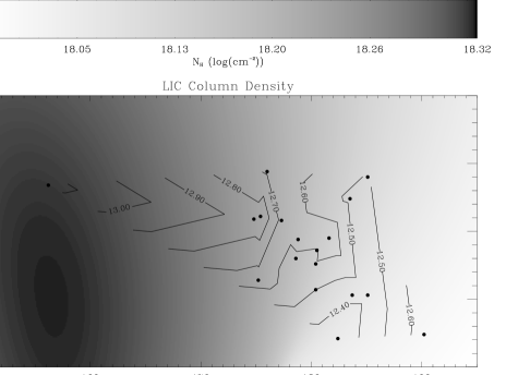
Figure 11: Contours of the Mg II column density of the LIC towards the Hyades stars, compared with the H I column density predicted by a model of the LIC [34], which is indicated by shading. The Mg II gradient is consistent with the H I gradient [48].

The consistency of the Mg II gradient with the expected LIC gradient in Figure 11 is further support for that component actually being LIC. This additional support is useful because the centroid velocities of the LIC components observed towards the Hyades are not exactly what the LIC vector predicts they should be. Figure 12 plots the observed velocities of the LIC components seen towards the Hyades stars versus the velocities predicted by the LIC vector. The Hyades stars are almost directly in the downwind direction relative to the LIC vector, so one would have expected to see LIC velocities close to 26 km s^-1, but the observed velocities are too low by about 3 km s^-1 on average. This discrepancy mirrors the discrepancy observed in the upwind direction towards 36 Oph, where the observed velocity is 3 km s^-1 too high. The interpretation for the upwind discrepancy was the existence of a distinct G cloud in that direction. However, the existence of a similar discrepancy downwind but with the observed velocities being too low instead of too high suggests that maybe we are detecting a velocity gradient within the LISM. The suggested gradient implies faster velocities upwind and slower velocities downwind, meaning the LISM material is being compressed. Perhaps this general LISM velocity gradient extends even further to the Hyades cloud, which is further downwind and does in fact appear to be slower than what we have been calling the LIC and G clouds.

Figure 12: Comparison of the observed velocity of the LIC component observed towards the Hyades stars with the value predicted by the LIC flow vector, showing that the observed velocities are too low by $\sim 3$ km s^-1 on average.

The Hyades data appear to call into question the reality of a G cloud that is a physically distinct entity from the LIC, and it also calls into question the interpretation of other supposedly non-LIC LISM components; the second component seen towards 61 Cyg in Figure 3, for example. The LIC component in Figure 3 is the one at $-9$ km s^-1. Is the second, redshifted component really a separate cloud, or is there a velocity gradient within the LIC that is responsible for the asymmetry in the Mg II absorption lines that leads to an erroneous two component interpretation? A useful exercise for the future will be to try to refine the LIC vector to see if it can be altered to be consistent with the Hyades velocities, while still preserving agreement with LIC velocities measured for other lines of sight. If this exercise is unsuccessful, it may be necessary to abandon the notion of LISM clouds with uniform flow vectors, which would greatly complicate interpretaions of LISM absorption line data.

3.4 Unusual Lines of Sight

There are a few lines of sight observed by HST that suggest that there is some nearby interstellar material with properties atypical for the LISM. These observations further serve to illustrate the complexity of LISM structure, and so we now briefly discuss these unusual lines of sight.

3.4.1 HD 82558

With a measured H I column of $\log N({\rm H~{}I})=19.05\pm 0.15$, the 18.3 pc line of sight to the K2 V star HD 82558 may have the highest average density yet observed within the LISM, $n({\rm H~{}I})\approx 0.2$ cm^-3 [22]. Very large column densities have also been observed towards the nearby ($d=14.3$ pc) A star $\alpha$ Oph [49], but much of this absorption may be circumstellar, as many A stars are surrounded by circumstellar material [50]. The $n({\rm H~{}I})\approx 0.2$ cm^-3 average density observed towards HD 82558 is only a factor of 2 higher than the average LIC density quoted in section 3.1 ($n({\rm H~{}I})=0.1$ cm^-3), but this average towards HD 82558 is computed assuming that the H I is evenly distributed along the entire 18.3 pc line of sight to HD 82558, which is very unlikely. High column densities have not been detected for any other nearby star in the general direction of HD 82558, meaning that the cloud responsible for the absorption is probably neither very large nor very close. Thus, the H I encountered towards HD 82558 that is producing so much absorption probably does not occupy a large fraction of the line of sight, and the actual density of the H I is probably more like $n({\rm H~{}I})\geq 0.5$ cm^-3, significantly higher than average densities within the LIC or G clouds. What makes this high density line of sight even more noteworthy is that HD 82558 is only $39^{\circ}$ from the “interstellar tunnel” towards $\epsilon$ CMa [51], where column densities are an order of magnitude lower towards stars an order of magnitude farther away [22]!

3.4.2 $\beta$ Ceti

The $\beta$ Ceti line of sight is remarkable for having a very high magnesium abundance [18]. Metal abundances within the LISM are generally found to be lower than solar, presumably due to depletion of metals onto dust grains [52]. A crude Mg abundance can be defined for a line of sight as ${\rm A(Mg)}\equiv N({\rm Mg~{}II})/N({\rm H~{}I})$. This assumes that Mg II is the dominant ionization state of Mg (probably a good assumption) and H I is the dominant ionization state of H (probably only good to within a factor of 2 — see section 3.1). A logarithmic depletion quantity can then be defined as ${\rm D(Mg)}\equiv\log{\rm A(Mg)}-\log{\rm A(Mg)_{\odot}}$, where ${\rm A(Mg)_{\odot}}=-4.41$ is the solar Mg abundance [53]. Typical values for the LIC are ${\rm D(Mg)}\approx-1.2$ [18, 21], meaning Mg in the LIC is underabundant by a factor of 15 due to depletion onto dust grains. Depletions are lower in the G cloud (see section 3.2), with ${\rm D(Mg)}\approx-0.6$ [10, 46].

However, the 29 pc line of sight to the K0 III star $\beta$ Cet has a remarkable depletion value of ${\rm D(Mg)}=+0.30\pm 0.15$, suggesting that if anything Mg is overabundant rather than depleted [18]. Significant ionization of H could at least remove the appearance of overabundance, but it seems clear that Mg is not significantly depleted towards $\beta$ Cet. The reason for this remains a mystery. We can only speculate that perhaps shocks in that direction have dissociated the dust grains and released all the previously depleted Mg back into the gas phase. Finally, we note that at least 2 and perhaps 3 velocity components are observed towards $\beta$ Cet, with the dominant component being at the velocity predicted by the LIC vector. However, this component’s identification with the LIC is questionable considering the wildly discrepant D(Mg) value.

3.4.3 70 Ophiuchi

Figure 13 shows the Mg II absorption observed towards 70 Oph, a K0 V star only 5.1 pc away that is close to the previously discussed 36 Oph line of sight in both distance and direction (see Fig. 7). Like 36 Oph, 70 Oph shows strong absorption at the position predicted by the G cloud vector, although the column toward 70 Oph is significantly higher. However, for 70 Oph there are two additional absorption components blueward of the saturated G cloud component. It is not unheard of to see multiple velocity components towards stars even as close as 70 Oph, but the velocity components are generally separated by less than 10 km s^-1. However, for the most blueshifted absorption component towards 70 Oph, the separation from the main component is about 18 km s^-1. This suggests that at least for this one line of sight there is apparently some LISM material with a velocity vector significantly different from the LIC and G cloud vectors. The origin of this anomalously fast LISM absorption component is unknown.

Figure 13: Three-component fits to the LISM Mg II h & k absorption lines observed towards 70 Oph, with the individual components shown as dotted lines and the combination of the two components shown as thick solid lines (after convolution with the instrumental profile).

4 HELIOSPHERIC AND ASTROSPHERIC ABSORPTION

One of the primary applications of LISM studies is to better understand how the LISM interacts with the winds of the stars contained within it, including our own Sun. It turns out that the same HST H I Ly$\alpha$ data that is used to study the LISM can also be used to study both the heliospheric interaction region surrounding our Sun and analogous “astrospheric” interaction regions around other nearby stars. Figure 14 shows the H I density and temperature within the heliosphere based on a hydrodynamic model [54, 55]. The heliopause (i.e., the contact surface separating the solar wind and ISM plasma flows) and bow shock are both visible at about 120 AU and 230 AU, respectively, in the upwind direction. Interstellar H I crossing the bow shock is heated by charge exchange processes [54, 56, 57]. This heated heliospheric hydrogen produces a substantial amount of Lyman-alpha absorption, enough to be detectable in HST data despite being highly blended with the LISM absorption. Analogous material around other solar-like stars has also been detected.

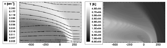
Figure 14: The H I density (left) and temperature (right) within the heliosphere predicted by a hydrodynamic model of the ISM–solar wind interaction, with streamlines shown in the left panel. The heliopause and bow shock are both visible at about 120 AU and 230 AU, respectively, in the upwind direction.

The four panels in the middle of Figure 15 show schematically what happens to a stellar Ly$\alpha$ emission profile as it travels from the star towards the Sun. (This particular example is modeled on the $\alpha$ Cen line of sight.) The Ly$\alpha$ profile first has to traverse the hot hydrogen in the star’s astrosphere which erases the central part of the line. The Ly$\alpha$ emission then makes the long interstellar journey, resulting in additional absorption, including some D I absorption. Finally, the profile has to travel through the hot hydrogen in the heliosphere, which results in additional absorption on the red side of the line. The reason the heliospheric absorption is redshifted is because of the deceleration of interstellar material as it crosses the bow shock. Conversely, astrospheric absorption will be blueshifted relative to the ISM absorption since we are viewing that absorption from outside the astrosphere rather than inside.

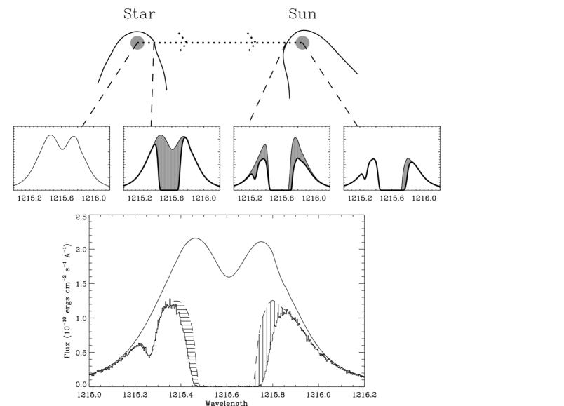
Figure 15: Schematic diagram showing how a stellar Ly$\alpha$ profile changes from its initial appearance at the star and then through various regions that absorb parts of the profile before it reaches an observer at Earth: the stellar astrosphere, the LISM, and finally the heliosphere. The lower panel shows the actual observed Ly$\alpha$ profile of $\alpha$ Cen B. The upper solid line is the assumed stellar emission profile and the dashed line is the ISM absorption alone. The excess absorption is due to heliospheric H I (vertical lines) and astrospheric H I (horizontal lines).

The bottom panel of Figure 15 shows the observed Ly$\alpha$ profile of $\alpha$ Cen B [10]. The upper solid line is the assumed stellar line profile. The dashed line is the LISM absorption alone, which is determined by forcing the interstellar H I absorption to have a Doppler parameter and central velocity consistent with D I and other LISM lines (see section 2.1). There is excess absorption on both sides of the LISM absorption, which cannot be accounted for by the single LISM component (G cloud) observed towards $\alpha$ Cen. The red side excess is best interpreted as heliospheric absorption and the blue side excess is best interpreted as astrospheric absorption [10, 58].

Heliospheric absorption has been detected towards three stars: $\alpha$ Cen [10], Sirius [59], and 36 Oph [46]. Comparisons with heliospheric models have shown that the observed heliospheric H I absorption is consistent with the predictions of the hydrodynamic models, and can potentially be used as a diagnostic for various input parameters for the models [46, 58, 59], such as the uncertain pressure provided by cosmic rays and the interstellar magnetic field. Astrospheric absorption has by now been detected towards seven stars, which are listed in Table 1, although the $\lambda$ And and 40 Eri A detections should be regarded as tentative [21, 60]. These astrospheric detections represent the first detections of winds analogous to the solar wind from solar-like main sequence stars.

Table 1: Compilation of Astrospheric Detections

Star	Spectral	$d$	$V_{ISM}$	$\theta$	Reference
	Type	(pc)	(km s-1)	(deg)
$\alpha$ Cen	G2 V+K0 V	1.3	25	79	[10]
$\epsilon$ Eri	K1 V	3.2	27	76	[17]
61 Cyg	K5 V+K7 V	3.5	86	46	[21]
$\epsilon$ Ind	K5 V	3.6	68	64	[60]
40 Eri A	K1 V	5.0	127	59	[21]
36 Oph	K1 V+K1 V	5.5	40	134	[46]
$\lambda$ And	G8 IV-III+?	26	53	89	[60]

The wind speed ($V_{ISM}$) and orientation angle relative to the Sun-star line of sight ($\theta$) of the LISM wind vector seen by each star can be computed from our knowledge of the LIC and/or G cloud flow vectors and the known proper motion and radial velocity of these stars. An example of this is illustrated in Figure 7 for the case of 36 Oph. The $V_{ISM}$ and $\theta$ values for each star with detected astrospheric absorption are listed in Table 1. The astrospheric observations show that the temperature of the astrospheric material is clearly higher for stars with faster $V_{ISM}$ values, consistent with theoretical expectations since a higher ISM wind speed will result in more shock heating at the bow shock [21].

With knowledge of $V_{ISM}$ and $\theta$ for a star, one can compute hydrodynamic models of the astrosphere analogous to the heliospheric model shown in Figure 14, and estimate predicted Ly$\alpha$ absorption from these models. The amount of absorption will depend on the mass loss rate assumed for the star. The larger the mass loss rate, the larger the astrosphere, and the higher the astrospheric H I column density. Thus, the astrospheric absorption can be used to obtain the first estimates of mass-loss rates for nearby solar-like stars [61, 62, 63].

Figure 16 reproduces the $\alpha$ Cen B spectrum from Figure 15 and compares the observed astrospheric absorption with the predictions of four models assuming four different mass-loss rates. The model assuming twice the solar mass-loss rate best fits the data. Since $\alpha$ Cen is actually a binary star consisting of two very solar-like stars with a combined surface area about twice that of the Sun, this result is very reasonable [61].

Figure 16: The $\alpha$ Cen B spectrum (thin solid line) and inferred ISM absorption (dotted line) are compared with a lower resolution STIS spectrum of $\alpha$ Cen’s distant companion Proxima Cen (thick solid line). The dashed lines show the blue-side excess Ly$\alpha$ absorption predicted by four models of the Alpha/Proxima Cen astrospheres, assuming four different mass loss rates. The $2.0~{}\dot{M}_{\odot}$ model fits the $\alpha$ Cen spectrum reasonably well, and the $0.2~{}\dot{M}_{\odot}$ model represents an upper limit for the mass loss rate of Proxima Cen [61].

Also shown in Figure 16 is the Ly$\alpha$ line observed towards Proxima Cen, a distant companion to the two $\alpha$ Cen stars that will not lie within the $\alpha$ Cen astrosphere. The LISM absorption should be the same, however, and the nearly identical amounts of D I absorption observed towards $\alpha$ Cen and Proxima Cen suggests that this is the case. (The Proxima Cen data have somewhat lower spectral resolution, which explains why the the Proxima Cen D I profile is somewhat broader and shallower.) The blue-side excess absorption observed towards $\alpha$ Cen that is being interpreted as astrospheric absorption is not observed towards Proxima Cen, which conclusively demonstrates that the excess absorption towards $\alpha$ Cen must in fact be circumstellar. If the excess was somehow due to LISM or heliospheric material it should have been observed towards both stars.

There is no detected astrospheric absorption towards Proxima Cen, and the model predictions shown in Figure 16 suggest an upper limit for the Proxima Cen mass loss rate of a fifth the solar value [61]. A low mass loss rate for Proxima Cen is not surprising in that Proxima Cen is a tiny, dim star with a surface area 40 times lower than that of the Sun. However, Proxima Cen does have a surprisingly active corona, with frequent large flares, so it was not obvious a priori that it would have a weak wind.

In principle, mass-loss rates can be estimated for all the stars in Table 1. A mass-loss rate of 0.5 solar has been estimated for $\epsilon$ Ind and a rate of 5 times solar has been estimated for $\lambda$ And [62, 63]. Estimates for the other stars will surely follow. Such studies, if expanded to include a sufficient number of stars, could allow us for the first time to see how mass-loss varies with stellar activity, age, spectral type, etc. As a final comment, it is remarkable that high resolution Ly$\alpha$ spectra of nearby stars are relevant to studies of such a wide variety of topics: stellar chromospheres, D/H and its implications for cosmology and Galactic chemical evolution, the structure and properties of the LISM in general, heliospheric physics, and, as just discussed, stellar winds which are otherwise undetectable.

References

- [1] D.M. Sfeir, R. Lallement, F. Crifo, and B.Y. Welsh, A&A 346 (1999) 785.
- [2] H.J. Fahr, Space Sci. Rev. 15 (1974) 483.
- [3] D.P. Cox and R.J. Reynolds, Ann. Rev. Astron. Astrophys. 25 (1987) 303.
- [4] A.K. Dupree, S.L. Baliunas, and H.L. Shipman, ApJ 218 (1977) 361.
- [5] W.B. Landsman, R.C. Henry, H.W. Moos, and J.L. Linsky, ApJ 285 (1984) 801.
- [6] W.B. Landsman, J. Murthy, R.C. Henry, H.W. Moos, J.L. Linsky, and J.L. Russell, ApJ 303 (1986) 791.
- [7] J. Murthy, R.C. Henry, H.W. Moos, W.B. Landsman, J.L. Linsky, A. Vidal-Madjar, and C. Gry, ApJ 315 (1987) 675.
- [8] J. Murthy, R.C. Henry, H.W. Moos, A. Vidal-Madjar, J.L. Linsky, and C. Gry, ApJ 356 (1990) 223.
- [9] P.R. McCullough, ApJ 390 (1992) 213.
- [10] J.L. Linsky and B.E. Wood, ApJ 463 (1996) 254.
- [11] T.P. Walker, Steigman, G., D.N. Schramm, K.A. Olive, and H.-S. Kang, ApJ 376 (1991) 51.
- [12] G. Steigman and M. Tosi, ApJ 401 (1992) 150.
- [13] E. Vangioni-Flam, K.A. Olive, and N. Prantzos, ApJ 427 (1994) 618.
- [14] S. Burles, K.M. Nollett, and M.S. Turner, ApJ 552 (2001) L1.
- [15] J.L. Linsky, et al., ApJ 402 (1993) 694.
- [16] J.L. Linsky, A. Diplas, B.E. Wood, A. Brown, T.R. Ayres, and B.D. Savage, ApJ 451 (1995) 335.
- [17] A.R. Dring, J.L. Linsky, J. Murthy, R.C. Henry, W. Moos, A. Vidal-Madjar, J. Audouze, and W. Landsman, ApJ 488 (1997) 760.
- [18] N. Piskunov, B.E. Wood, J.L. Linsky, R.C. Dempsey, and T.R. Ayres, ApJ 474 (1997) 315.
- [19] J.L. Linsky, Space Sci. Rev. 84 (1998) 285.
- [20] P. Bertin, A. Vidal-Madjar, R. Lallement, R. Ferlet, and M. Lemoine, A&A 302 (1995) 889.
- [21] B.E. Wood and J.L. Linsky, ApJ 492 (1998) 788.
- [22] B.E. Wood, C.W. Ambruster, A. Brown, and J.L. Linsky, ApJ 542 (2000) 411.
- [23] A. Vidal-Madjar, et al., A&A 338 (1998) 694.
- [24] E.B. Jenkins, T.M. Tripp, P.R. Wozniak, U.J. Sofia, and G. Sonneborn, ApJ 520 (1999) 182.
- [25] G. Sonneborn, T.M. Tripp, R. Ferlet, E.B. Jenkins, U.J. Sofia, A. Vidal-Madjar, and P.R. Wozniak, ApJ 545 (2000) 277.
- [26] R. Lallement, P. Bertin, R. Ferlet, A. Vidal-Madjar, and J.L. Bertaux, A&A 286 (1994) 898.
- [27] R. Lallement, R. Ferlet, A.M. Lagrange, M. Lemoine, and A. Vidal-Madjar, A&A 304 (1995) 461.
- [28] J.L. Bertaux and J.E. Blamont, A&A 11 (1971) 200.
- [29] E. Quémerais, J.-L. Bertaux, R. Lallement, M. Berthé, E. Kyrölä, and W. Schmidt, JGR 104 (1999) 12,585.
- [30] E. Quémerais, J.-L. Bertaux, R. Lallement, M. Berthé, E. Kyrölä, and W. Schmidt, Adv. Space Res. 26 (2000) 815.
- [31] M. Witte, H. Rosenbauer, M. Banaszkewicz, and H. Fahr, Adv. Space Res. 13 (1993) 121.
- [32] M. Witte, M. Banaszkewicz, and H. Rosenbauer, Space Sci. Rev. 78 (1996) 289.
- [33] R. Lallement and P. Bertin, A&A 266 (1992) 479.
- [34] S. Redfield and J.L. Linsky, ApJ 534 (2000) 825.
- [35] E. Quémerais, J.-L. Bertaux, B.R. Sandel, and R. Lallement, A&A 290 (1994) 941.
- [36] V.V. Izmodenov, J. Geiss, R. Lallement, G. Gloeckler, V.B. Baranov, and Y.G. Malama, JGR 104 (1999) 4731.
- [37] P.C. Frisch, Science 265 (1994) 1423.
- [38] R. Lallement and R. Ferlet, A&A 324 (1997) 1105.
- [39] C.-H. Lyu and F.C. Bruhweiler, ApJ 459 (1996) 216.
- [40] F.C. Bruhweiler and K.-P. Cheng, ApJ 335 (1988) 188.
- [41] K.-P. Cheng and F.C. Bruhweiler, ApJ 364 (1990) 573.
- [42] B.E. Wood and J.L. Linsky, ApJ 474 (1997) L39.
- [43] J. Dupuis, S. Vennes, S. Bowyer, A.K. Pradhan, and P. Thejll, ApJ 455 (1995) 574.
- [44] J.B. Holberg, M.A. Barstow, F.C. Bruhweiler, and E.M. Sion, ApJ 453 (1995) 313.
- [45] T. Lanz, M.A. Barstow, I. Hubeny, and J.B. Holberg, ApJ 473 (1996) 1089.
- [46] B.E. Wood, J.L. Linsky, and G.P. Zank, ApJ 537 (2000) 304.
- [47] S. Grzedzielski and R. Lallement, Space Sci. Rev. 78 (1996) 247.
- [48] S. Redfield and J.L. Linsky, ApJ 551 (2001) 413.
- [49] P.C. Frisch, D.G. York, and J.R. Fowler, ApJ 320 (1987) 842.
- [50] H. Holweger, M. Hempel, and I. Kamp, A&A 350 (1999) 611.
- [51] C. Gry, L. Lemonon, A. Vidal-Madjar, M. Lemoine, and R. Ferlet, A&A 302 (1995) 497.
- [52] P.C. Frisch, et al., ApJ 525 (1999) 492.
- [53] E. Anders and N. Grevesse, Geochim. Cosmochim. Acta 53 (1989) 197.
- [54] G.P. Zank, H.L. Pauls, L.L. Williams, and D.T. Hall, JGR 101 (1996) 21,639.
- [55] B.E. Wood, H.-R. Müller, and G.P. Zank, ApJ 542 (2000) 493.
- [56] V.B. Baranov and Y.G. Malama, JGR 98 (1993) 15,157.
- [57] V.B. Baranov and Y.G. Malama, JGR 100 (1995) 14,755.
- [58] K.G. Gayley, G.P. Zank, H.L. Pauls, P.C. Frisch, and D.E. Welty, ApJ 487 (1997) 259.
- [59] V.V. Izmodenov, R. Lallement, and Y.G. Malama, A&A 342 (1999) L13.
- [60] B.E. Wood, W.R. Alexander, and J.L. Linsky, ApJ 470 (1996) 1157.
- [61] B.E. Wood, J.L. Linsky, H.-R. Müller, and G.P. Zank, ApJ 547 (2001) L49.
- [62] H.-R. Müller, G.P. Zank, and B.E. Wood, ApJ 551 (2001) 495.
- [63] H.-R. Müller, G.P. Zank, and B.E. Wood, The Outer Heliosphere: The Next Frontiers (2001) in press.