[

Probing the Dark Energy with Quasar Clustering

Abstract

We show, through Monte Carlo simulations, that the Alcock-Paczyński test, as applied to quasar clustering, is a powerful tool to probe the cosmological density and equation of state parameters, $\Omega_{m0}$, $\Omega_{x0}$ and $w$. By taking into account the effect of peculiar velocities upon the correlation function we obtain, for the Two-Degree Field QSO Redshift Survey (2QZ), the predicted confidence contours for the cosmological constant ($w=-1$) and spatially flat ($\Omega_{m0}+\Omega_{x0}=1$) cases. It turns out that, for $w=-1$, the test is especially sensitive to the difference $\Omega_{m0}-\Omega_{\Lambda 0}$, thus being ideal to combine with CMB results. We also find out that, for the flat case, it is competitive with future supernova and galaxy number count tests, besides being complementary to them.

]

Introduction.

Recent investigations of type Ia supernovae (SNe Ia) suggest that the expansion of the Universe is accelerating, driven by some kind of negative-pressure dark energy [1, 2]. Independent evidence for the SNe Ia results is provided by observations of cosmic microwave background (CMB) anisotropies in combination with constraints on the matter density parameter ($\Omega_{m0}$) [3]. The exact nature, however, of this dark energy is not well understood at present. Vacuum energy or a cosmological constant ($\Lambda$) is the simplest explanation, but attractive alternatives like a dynamical scalar field (quintessence) [4] have also been explored in the literature. An important task nowadays in cosmology is thus to find new methods that could directly quantify the amount of dark energy present in the Universe as well as determine its equation of state and time dependence. New methods may constrain different regions of the parameter space and are usually subject to different systematic errors, and they are therefore crucial to cross-check (or complement) the SNe results.

The test we focus on here is the one suggested by Alcock and Paczyński (hereafter AP)[5], which has attracted a lot of attention during the last years [6, 7, 8, 9, 10]. In particular, Popowski et al. [11] (hereafter PWRO) extended a calculation by Phillips [12] of the geometrical distortion of the QSO correlation function. They suggested a simple Monte Carlo experiment to see what constraints should be expected from the 2dF QSO Redshift Survey (2QZ) and the Sloan Digital Sky Survey (SDSS). However, they did not estimate the probability density in the parameter space and, as a consequence, they could not notice that the test is in fact very sensitive to the difference $\Omega_{m0}-\Omega_{\Lambda 0}$. Further, they did not take into account the effect of peculiar velocities, although they discussed its role arguing that it would not overwhelm the geometric signal.

Our aim, in this Letter, is to show the feasibility of redshift distortion (geometric + peculiar velocity) measurements to constrain cosmological parameters, by extending the PWRO Monte Carlo experiments and obtaining confidence regions in the ($\Omega_{m0},\Omega_{\Lambda 0}$) and ($\Omega_{m0},w$) planes. We compare the expected constraints from the AP test, when applied to the 2QZ survey, with those obtained by other methods. We include a general dark energy component with equation of state $P_{x}=w\,\rho_{x}$, with $w$ constant. Our analysis can be generalized to dynamical scalar field cosmologies as well as to any model with redshift dependent equation of state. Since most quasars have redshift $z\lesssim 2$ we expect the test to be useful in the determination of a possible redshift dependence of the equation of state. We explicitly take into account the effect of large-scale coherent peculiar velocities. Our calculations are based on the measured 2QZ distribution function and we consider best fit values for the amplitude ($r_{0}$) and exponent ($\gamma$) of the correlation function as obtained by Croom et al. [13]. In this work, we only consider the 2QZ survey although the results can easily be generalized to SDSS.

Alcock-Paczyński test and quasar clustering. We assume that the geometry is described by the standard Robertson-Walker metric. By a straightforward calculation for null geodesics, we obtain the radial coordinate $R$ as a function of $z$:

$$a_{0}R=g(z):=\left\{\begin{array}[]{lr}\sinh(\sqrt{\Omega_{k0}}I(z))/(H_{0}\sqrt{\Omega_{k0}}),\;\Omega_{k0}>0,\\ I(z),\;\Omega_{k0}=0,\\ \sin(\sqrt{-\Omega_{k0}}I(z))/(H_{0}\sqrt{-\Omega_{k0}}),\;\Omega_{k0}<0,\end{array}\right.$$ (1)

where $a_{0}$ is the present scale factor, $I(z):=\int_{z^{\prime}=0}^{z}[H_{0}/H(z^{\prime})]dz^{\prime}$, and the Hubble parameter is given by $H(z)=H_{0}[\Omega_{m0}(1+z)^{3}+\Omega_{x0}(1+z)^{3(1+w)}+\Omega_{k0}(1+z)^{2}]^{1/2}$.

Given two close point sources (e.g., quasars), with coordinates $(z,\theta,\phi)$ and $(z+dz,\theta+d\theta,\phi+d\phi)$, directly read off a catalogue, the real-space infinitesimal comoving distance between them can be decomposed, in the distant observer approximation we adopt, into contributions parallel and perpendicular to the line of sight, $r_{\perp}:=g(z)d\alpha$, $r_{||}:={dz}/{H(z)}$, such that $r^{2}=r_{||}^{2}+r_{\perp}^{2}$. Here, $d\alpha$ is the small angle between the lines of sight.

The gist of the AP test relies then on the fact that, if we observe an intrinsically spherical system ($r_{||}=r_{\perp}$), it will appear distorted, in redshift space, according to the generic formula ${r_{\perp}}/{r_{||}}=j(z){s_{\perp}}/{s_{||}},$ where the anisotropy or distortion function $j(z)$ is defined by $j(z):={g(z)H(z)}/{z}.$ Here we have assumed a Euclidean geometry for redshift space, that is, $s_{||}:=dz$, $s_{\perp}:=zd\alpha$, and $s^{2}=s_{||}^{2}+s_{\perp}^{2}$.

Observations [13] suggest that, on scales $\sim 1-40h^{-1}$ Mpc, the real space correlation function for quasars is reasonably well fitted by a power law, $\xi(r)=\left({r}/{r_{0}}\right)^{-\gamma}$, which leads, in redshift space, to an anisotropic correlation function, $\xi(s,\mu)=\left[{s}/{s_{0}(z)}\right]^{-\gamma}\left[{\mu^{2}+j^{2}(z)(1-\mu^{2})}\right]^{-\gamma/2}$, where $\mu:=s_{||}/s$ and $s_{0}(z):=r_{0}H(z).$

Peculiar velocities also induce distortions in the correlation function which can be confused with those arising from the cosmological geometric effect. It is important to take them into account when comparing theory with observations. For the $(z,s)$ range we will consider, the influence of small-scale velocity dispersions is likely to be weak [11] and we neglect it in our analysis. The most relevant effect to be considered is due to large-scale coherent flows [14]. The linear theory correlation function is given by [15, 8]

$$\xi_{L}(s,\mu)=\left[\left(1+\frac{2\beta}{3}+\frac{\beta^{2}}{5}\right)P_{0}(\overline{\mu})+\left(\frac{4\beta}{3}+\frac{4\beta^{2}}{7}\right)\right.$$ (2)

$$\left.\times\frac{\gamma}{\gamma-3}P_{2}(\overline{\mu})+\frac{8\beta^{2}}{35}\frac{\gamma(\gamma+2)}{(5-\gamma)(3-\gamma)}P_{4}(\overline{\mu})\right]\xi(r),$$ (3)

where the $P_{i}(\overline{\mu})$ are Legendre polynomials, and $\overline{\mu}:=r_{||}/r$. As usual, $\beta(z):={f(z)}/{b(z)}$, $f(z):=-d\ln D/d\ln(1+z)$ is the linear growth rate, and we adopt the following dependence for the bias parameter, $b(z)=1+\left[D(z=0)/{D(z)}\right]^{m}\left(b_{0}-1\right).$ If $m=1$, we have Fry’s number-conserving bias model [16]. The case $m=0$ corresponds to a constant bias, and we also use $m\simeq 1.7$ in our computations, which seems to be more in accordance with an observed nonevolving clustering [13]. For models where the dark energy is a cosmological constant ($w=-1)$, we use the Heath solution for the growing mode [17], $D(z)=\frac{5}{2}\Omega_{m0}H(z)\int_{z}^{\infty}{(1+x)}/{H(x)^{3}}dx,$ and the following approximation for the growth rate [18], $f(z)\simeq\Omega_{m}^{4/7}(z)+\frac{1}{70}{\Omega_{\Lambda}(z)}\left[1+{\Omega_{m}(z)}/{2}\right].$ For flat models, Silveira and Waga [19] obtained an exact solution for the growing mode, $D(z)={{}_{2}F}_{1}\left[-\frac{1}{3w},\frac{w-1}{2},1-\frac{5}{6w};\frac{1-\Omega_{m0}}{\Omega_{m0}}(1+z)^{3w}\right]/(1+z)$, where ${}_{2}F_{1}[a,b,c;x]$ is the hypergeometric function. The growth rate can also be expressed in terms of hypergeometric functions.

Following PWRO, we obtain, for the number of pairs expected in an infinitely small bin within ($z,s,\mu$) and ($z+dz,s+ds,\mu+d\mu$),

$$dN_{pairs}=-\frac{2\pi}{A}\!\left(\frac{180\,N_{Q}\,F(z)}{\pi\,z}\right)^{\!2}\![1+\xi_{L}(s,\mu)]\,s^{2}dz\,ds\,d\mu.$$ (4)

Here $A$ is the area (in deg²) of the survey, $N_{Q}$ is the total number of sources (quasars) in the survey, and $F(z)$ is the normalized distribution function.

Croom et al. [13], assuming an Einstein-de Sitter Universe ($\Omega_{m}=1,\Omega_{\Lambda}=0$), showed that the quasar clustering amplitude $r_{0}$ appears to vary very little over the entire redshift range of the 2QZ survey. They found $r_{0}\simeq 4\,h^{-1}$ Mpc as their best fit, which remains nearly constant in comoving coordinate. Therefore, we have $s_{0}|_{EdS}(z):=H(z)|_{EdS}\,{r_{0}}=({4}/{3000})(1+z)^{3/2}.$ Following again PWRO, we use the fact that the total number of correlated pairs, $N_{pairs}$, in the survey is model independent to scale $s_{0}(z)$ to other cosmologies. It is straightforward to show that $N_{pairs}\propto{s_{0}^{3}(z)}/{j^{2}(z)}$, and we use $s_{0}(z)=({4}/{3000})(1+z)^{3/2}\left[{j(z)}/{j|_{EdS}(z)}\right]^{2/3}$ as a fiducial redshift-space correlation length for our simulations.

A particular model predicts a number of pairs $A_{i}$ in each bin of a $(z,s,\mu)$ space. In a real (or simulated) situation the data consist of $N_{i}$ pairs in $i$ bins. PWRO showed that for typical surveys, such as SDSS and 2QZ, we are bound to be in the “sparse regime” or “Poisson limit”. In this case we may treat bins in $(z,s,\mu)$ space as independent and the probability of detecting $N_{i}$ pairs in bin $i$, when $A_{i}$ are expected, is $P(N_{i}|A_{i})={e^{-A_{i}}A_{i}^{N_{i}}}/{N_{i}!}$ Since the bins are independent, the likelihood ${\cal L}$ of obtaining the data given the model is simply the product, ${\cal L}=\prod_{i}P(N_{i}|A_{i})$. For a typical 2QZ simulation, we assumed: (i) the completed survey will comprise $N_{Q}=26000$ quasars in a total area $A=750$ deg²; (ii) the Einstein-de Sitter fiducial correlation function has $r_{0}=4h^{-1}$ Mpc and $\gamma=1.6$; (iii) the bias model is determined by $b_{0}=1.5$ and $m=1$. The linear binning we chose covered the ranges: $0.4<z<2.6$, $2<s/s_{0}(z)<7$, and $0<\mu<1$, with 16 bins in $z$, 25 in $s/s_{0}(z)$, and 5 in $\mu$, making up a total of 2000 bins. The maximization of the likelihood was carried out with minuit [20] and cross-checked with mathematica. The probability density function was built via a Gaussian kernel density estimate, from typically 1000 runs for each “true” model.

Results and discussion.

In Figure 1, we show the predicted AP likelihood contours in the ($\Omega_{m0},\Omega_{\Lambda 0}$)-plane for the 2QZ survey (solid lines), in the case $w=-1$, in a universe with arbitrary spatial curvature. The scattered points represent maximum likelihood best fit values for $\Omega_{m0}$ and $\Omega_{\Lambda 0}$. The assumed “true” values are ($\Omega_{m0}=0.3,\Omega_{\Lambda 0}=0$) and ($0.28,0.72$), for the top and bottom panels, respectively. In the top panel the displayed curve corresponds to the predicted $2\sigma$ likelihood contour. In the bottom panel the predicted $1\sigma$ contour (dashed line) for one year of SNAP data [21] is displayed, together with the predicted $1\sigma$ AP contour. For the SNAP contour, it is assumed that the intercept $\cal{M}$ is exactly known. To have some ground of comparison with current SNe Ia observations, in the same panel, we also plot (dotted lines) the Supernova Cosmology Project [2] $1\sigma$ contour (fit C). As expected, in both cases, the test recovers nicely the “true” values. We stress out that the test is very sensitive to the difference $\Omega_{m0}-\Omega_{\Lambda 0}$. From the bottom panel we note that the sensitivity to this difference is comparable to that expected from SNAP, of the order $\pm 0.01$. Comparatively, however, the test has a larger uncertainty in the determination of $\Omega_{m0}+\Omega_{\Lambda 0}$, of the order $\pm 0.21$. The degeneracy in $\Omega_{m0}+\Omega_{\Lambda 0}$ may be broken if we combine the estimated results for the AP test with, for instance, those from CMB anisotropy measurements, whose contour lines are orthogonal to those exhibited in the panels [22].

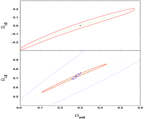
FIG. 1.: Simulated models at fixed $w=-1$ and corresponding predicted AP confidence contours (solid lines). In the top panel we show the predicted $2\sigma$ likelihood contour assuming a “true” model ($\Omega_{m0}=0.3,\Omega_{\Lambda 0}=0)$. In the bottom panel the predicted $1\sigma$ contour (dashed line) for one year of SNAP data [21] is displayed, together with the predicted $1\sigma$ AP contour. For both tests we consider $\Omega_{m0}=0.28$ and $\Omega_{\Lambda 0}=0.72$; also displayed is a $1\sigma$ confidence contour obtained by the Supernova Cosmology Project (dotted lines; [2]).

In order to estimate the consequences of neglecting the effect of linear peculiar velocities, in the top panel of Figure 2, we included them in the calculation of the $A_{i}$ values but neglected them in the computation of the maximum likelihood; in this panel, we assume $\Omega_{m0}=0.3$ and $\Omega_{\Lambda 0}=0$ as “true” values. Notice that the point with the “true” $\Omega_{m0}$ and $\Omega_{\Lambda 0}$ values is outside the $2\sigma$ contour. It is clear, therefore, the necessity of taking this effect in consideration when analyzing real data.

To illustrate that the AP test is in fact more sensitive to the mean amplitude of the bias rather than to its exact redshift dependence, we plot, in the bottom panel of Figure 2, the $2\sigma$ contour line, assuming as “true” values $\Omega_{m0}=0.3$ and $\Omega_{\Lambda 0}=0.7$. For this panel, the “true” $A_{i}$ values were generated assuming $b_{0}=1.45$ and $m=1.68$. However, for the simulations, we considered a constant bias ($m=0$), such that $b_{0,sim}:=\int_{z=z_{min}}^{z_{max}}F(z)b_{true}(z)dz=2.46$. We remark that the contour is slightly enlarged and shifted in the direction of the “ellipsis” major axis. However, the uncertainty in $\Omega_{m0}-\Omega_{\Lambda 0}$ is practically unaltered, confirming the strength of the test [23]. We did the same analysis assuming $\Omega_{m0}=1$ and $\Omega_{\Lambda 0}=0$ and obtained similar results.

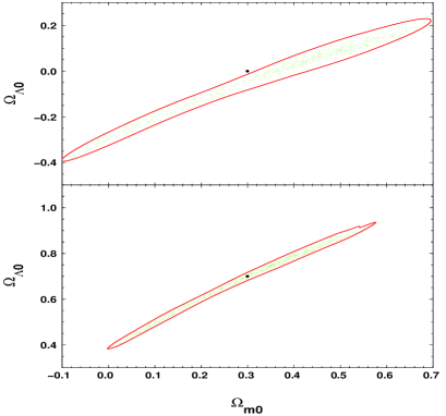
FIG. 2.: Simulated models at fixed $w=-1$ and corresponding $2\sigma$ predicted AP confidence contour; in both panels, the “true” model is indicated by a solid dot. Top panel: The “true” model, $(0.3,0)$, takes into account the effect of peculiar velocities, but the simulated ones do not. Notice that the “true” model does not fall into the $2\sigma$ confidence region. Bottom panel: The “true” model, $(0.3,0.7)$, uses a redshift dependent bias function with $b_{0}=1.45$ and $m=1.68$, whereas the simulated ones use a constant bias equal to 2.46.

In Figure 3, we show the predicted AP likelihood contours in the $(\Omega_{m0},w)$-plane for the 2QZ survey (solid lines) for flat models ($\Omega_{k0}=0$). The “true” values are $(\Omega_{m0}=0.28,w=-1)$ and $(\Omega_{m0}=0.3,w=-0.7)$ for the top and bottom panels, respectively. In the top panel, we show, besides the AP contour, the predicted contour for one year of SNAP data (dashed line; [21]), both at $1\sigma$ level. For the SNAP contour, the intercept $\cal{M}$ is assumed to be exactly known. Notice that the contours are somewhat complementary and are similar in strength. In the bottom panel, we compare the predicted $95\%$ confidence contour of the AP test with the same confidence contour for the number count test as expected from the DEEP redshift survey (dashed line; [24]). Again the contours are complementary, but the uncertainties on $\Omega_{m0}$ and $w$ for the AP test are quite smaller.

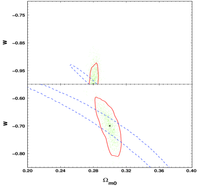
FIG. 3.: Simulated flat models and corresponding predicted AP confidence contours (solid lines). The top panel is from a “true” model ($\Omega_{m0}=0.28$, $w=-1$), and displays the predicted confidence contours for the AP test and the SNAP mission (dashed line; [21]), both at $1\sigma$ level. The bottom panel is from a “true” model ($\Omega_{m0}=0.3$, $w=-0.7$), and displays the predicted confidence contours for the AP test and the DEEP survey (dashed line; [24]), both at the $95\%$ level.

In summary, we have shown that the Alcock-Paczyński test applied to the 2dF quasar survey (2QZ) is a potent tool for measuring cosmological parameters. We stress out that the test is especially sensitive to $\Omega_{m0}-\Omega_{\Lambda 0}$. We have established that the expected confidence contours are in general complementary to those obtained by other methods and we again emphasize the importance of combining them to constrain even more the parameter space. We have also revealed that, for flat models, the estimated constraints are similar in strength to those from SNAP with the advantage that the 2QZ survey will soon be completed.

Of course our analysis can be improved in several aspects. For instance, for the fiducial Einstein-de Sitter model, we have assumed that $\gamma$ and $r_{0}$ do not depend on redshift. In fact, observations [13] seem to support these assumptions, but further investigations are necessary. Further, in the simulations, for Figure 1 and Figure 3, we have assumed that the parameters $r_{0}$, $\gamma$, $b_{0}$ and $m$ are known exactly, that is, they are the same as the “true” input ones. Marginalization over these parameters is expected to increase the size of the contours. However, preliminary results where the errors in $r_{0}$ and $\gamma$ are taken into account (supposed Gaussian), show that the confidence contours are not appreciably altered. At present, the quasar clustering bias is not completely well understood. Theoretical as well as observational progress in its determination will certainly improve the real capacity of the test. However, confirming previous investigations [23], we have found that the test is, in fact, more sensitive to the mean amplitude of the bias rather than to its exact redshift dependence. A more extensive report of this work and further investigations will be published elsewhere.

We would like to thank J. Silk for calling attention to the potential of the AP test and T. Kodama for suggestions regarding numerical issues. We also thank the Brazilian research agencies CNPq, FAPERJ and FUJB.

REFERENCES

- [1] A. G. Riess et al., AJ, 116, 1009 (1999).
- [2] S. Perlmutter et al., ApJ, 517, 565 (1999).
- [3] P. de Bernardis et al., Nature, 404, 955 (2000); A. Balbi et al., ApJ, 545, L1 (2000); C. Pryke et al., astro-ph/0104490; N. A. Bahcall, J. P. Ostriker, S. Perlmutter, and P. J. Steinhardt, Science, 284, 1481 (1999); M. S. Turner, Physica Scripta, T85, 210 (2000).
- [4] B. Ratra, and P. J. E. Peebles, Phys. Rev. D, 37, 3406 (1988); J. A. Frieman, C. T. Hill, A. Stebbins, and I. Waga, Phys. Rev. Lett., 75, 2077 (1995); R. R. Caldwell, R. Dave, and P. J. Steinhardt, Phys. Rev. Lett., 80, 1582 (1998); P. G. Ferreira, and M. Joyce, Phys. Rev. D, 58, 023503 (1998).
- [5] C. Alcock, and B. Paczyński, Nature, 281, 358 (1979) [AP].
- [6] B. S. Ryden, ApJ, 452, 25 (1995).
- [7] W. E. Ballinger, J. A. Peacock, and A. F. Heavens, MNRAS, 282, 877 (1996).
- [8] T. Matsubara, and Y. Suto, ApJ, 470, L1 (1996).
- [9] L. Hui, A. Stebbins, and S. Burles, ApJ, 511, L5 (1999).
- [10] P. McDonald, and J. Miralda-Escudé, ApJ, 518, 24 (1999).
- [11] P. A. Popowski, D. H. Weinberg, B. S. Ryden, and P. S. Osmer, ApJ, 498, 11 (1998) [PWRO].
- [12] S. Phillipps, MNRAS, 269, 1077 (1994).
- [13] S. M. Croom et al., MNRAS, 325, 483 (2001).
- [14] N. Kaiser, MNRAS, 227, 1 (1987).
- [15] A. J. S. Hamilton, ApJ, 385, L5 (1992).
- [16] J. N. Fry, ApJ, 461, L65 (1996).
- [17] D. J. Heath, MNRAS, 179, 351 (1977).
- [18] O. Lahav, P. B. Lijle, J. R. Primack, and M. J. Rees, MNRAS, 251, 136 (1991).
- [19] V. Silveira, and I. Waga, Phys. Rev. D, 50, 4890 (1994).
- [20] F. James, MINUIT Reference Manual Version 94.1, CERN Program Library Long Writeup D506, CERN (1994) .
- [21] M. Goliath, R. Amanullah, P. Astier, A. Goobar, and R. Pain, Astron. Astrophys., 380, 6 (2001) .
- [22] W. Hu, D. J. Eisenstein, M. Tegmark, and M. White, Phys. Rev. D, 59, 023512 (1999).
- [23] K. Yamamoto, and H. Nishioka, ApJ, 549, L15 (2001).
- [24] J. F. Newman, and M. Davis, ApJ, 534, L11 (2000).