Seyfert-Type Dependences of Narrow Emission-Line Ratios and
Physical Properties of High-Ionization Nuclear Emission-Line Regions
in Seyfert Galaxies

Abstract

In order to examine how narrow emission-line flux ratios depend on the Seyfert type, we compiled various narrow emission-line flux ratios of 355 Seyfert galaxies from the literature. We present in this paper that the intensity of the high-ionization emission lines, [Fe vii]$\lambda$6087, [Fe x]$\lambda$6374 and [Ne v]$\lambda$3426, tend to be stronger in Seyfert 1 galaxies than in Seyfert 2 galaxies. In addition to these lines, [O iii]$\lambda$4363 and [Ne iii]$\lambda$3869, whose ionization potentials are not high ($<$ 100 eV), but whose critical densities are significantly high ($\gtrsim 10^{7}$ cm^-3), also exhibit the same tendency. On the other hand, the emission-line flux ratios among low-ionization emission lines do not show such a tendency. We point out that the most plausible interpretation of these results is that the high-ionization emission lines arise mainly from highly-ionized, dense gas clouds, which are located very close to nuclei, and thus can be hidden by dusty tori. To examine the physical properties of these highly-ionized dense gas clouds, photoionization model calculations were performed. As a result, we find that the hydrogen density and the ionization parameter of these highly-ionized dense gas clouds are constrained to be $n_{\rm H}>10^{6}$ cm^-3 and $U>10^{-2}$, respectively. These lower limits are almost independent both from the metallicity of gas clouds and from the spectral energy distribution of the nuclear ionizing radiation.

1. Introduction

Seyfert nuclei are typical active galactic nuclei (AGNs) in the nearby universe. They have been broadly classified into two types based on the presence or absence of broad (typically $\gtrsim$ 2000 km s^-1) permitted emission lines in their optical spectra (Khachikian, Weedman 1974); Seyfert nuclei with broad lines are type 1 (hereafter S1), while those without broad lines are type 2 (S2). This difference is thought to be due to a dependence of the visibility of broad-line regions (BLRs) on the viewing angle. Accordingly, the BLR is thought to be located in a very inner region (a typical radial distance from the central black hole is $r\sim 0.01$ pc; see, e.g., Peterson 1993) and surrounded by a geometrically- and optically-thick dusty torus (AGN unified model; see Antonucci 1993 for a review).

Contrary to the BLR emission, narrow (typically $\lesssim$ 1000 km s^-1) permitted and forbidden emission lines, arising from narrow-line regions (NLRs), are seen in the spectra of both S1s and S2s. Therefore, the NLR is believed to be located far from the nucleus, and thus not to be hidden by dusty tori. If this is the case, the observed physical properties of ionized gas in NLRs do not depend on the viewing angle toward dusty tori. However, several studies have statistically shown that some high-ionization emission lines, such as [Fe vii]$\lambda$6087, [Fe x]$\lambda$6374, and [Ne v]$\lambda$3426, are stronger in spectra of S1s than in those of S2s (e.g., Shuder, Osterbrock 1981; Cohen 1983; Murayama, Taniguchi 1998a; Schmitt 1998; Nagao et al. 2000). Some emission lines whose ionization potential is not so high ($<$ 100 eV), but whose critical density is high, such as [O iii]$\lambda$4363 and [Ne iii]$\lambda$3869, also show the same Seyfert-type dependence (e.g., Osterbrock et al. 1976; Heckman, Balick 1979; Shuder, Osterbrock 1981; Schmitt 1998; Nagao et al. 2001b). These Seyfert-type dependences in some emission-line intensities seem to conflict with the framework of the AGN unified model. Therefore, some possible models have been proposed to explain such Seyfert-type dependences in the narrow emission-line intensities. One of the proposed ideas is that these Seyfert-type dependences in the strength of the high-ionization emission lines are caused by a viewing-angle dependence of the visibility of highly-ionized dense gas clouds, which are located very close to the nucleus, and thus can be hidden by dusty tori (Murayama, Taniguchi 1998a, b; Nagao et al. 2000, 2001b). On the contrary, Schmitt (1998) pointed out that the Seyfert-type dependences in the intensities of the high-critical-density transition can be understood if the intrinsic difference in the NLR size between S1s and S2s (see, e.g., Schmitt, Kinney 1996) is taken into account.

Which is the origin of the Seyfert-type dependence of those emission lines, the inclination effect (i.e., obscuration by dusty tori) or the intrinsic difference in the size of NLRs? To investigate this issue, it should be examined how emission-line strengths depend on the Seyfert-type. Thus, we have compiled emission-line flux ratios of many Seyfert galaxies from the literature. In this paper, we show the Seyfert-type dependence of various emission-line flux ratios based on this compiled database and discuss the origin of the Seyfert-type dependence.

2. The Data

2.1. Data

In this section, we briefly describe the properties of the database of emission-line flux ratios. See Nagao (2001) for details of this database. The database contains various emission-line flux ratios of 355 Seyfert nuclei in total; 33 narrow-line S1s (NLS1s; see, e.g., Osterbrock, Pogge 1985), 48 broad-line S1s (BLS1s), 48 Seyfert 1.2 galaxies (S1.2s), 78 Seyfert 1.5 galaxies (S1.5s), 9 Seyfert 1.8 galaxies (S1.8s), 28 Seyfert 1.9 galaxies (S1.9s), 6 S2s with broad emission in near-infrared spectra (S2_NIR-BLRs), 12 S2s with broad polarized emission (S2_HBLRs), and 93 S2s without any broad emission in their spectra (S2^-s). In this paper, S1.2s are basically included in BLS1s, and S1.8s, S1.9s, and S2_NIR-BLRs are gathered into the class of “S2 with reddened BLR (S2_RBLR)”. When necessary, NLS1s and BLS1s are gathered into the class of “S1_total”, and S2_RBLR, S2_HBLRs, and S2^-s are gathered into the class of “S2_total”. We adopt the classification of the Seyfert types by Véron-Cetty and Véron (2000).

Since it is often difficult to measure the flux of narrow Balmer components accurately for S1s (and S1.5s), the correction for dust extinction adopting the Balmer decrement method (see, e.g., Osterbrock 1989) would cause possible systematic errors. Therefore, we did not correct any dust extinction effect on the emission-line flux ratios in the database. The effects of dust extinction on the following discussion are mentioned in subsection 3.2.

2.2. Selection Biases

The sample used here is not a complete one in any sense. Therefore, it is necessary to check whether or not the sample is appropriate for the statistical and comparative investigations carried out in the following sections. Since some possible biases may be caused if there are large systematic differences in their redshift or intrinsic luminosity distributions, we check their distributions below.

First, we check the frequency distribution of redshift for each type of Seyfert galaxies. The histogram of the frequency distribution, the median, the average, and the 1 $\sigma$ deviation of the redshift for each type of Seyfert galaxies are presented in figure 1 and table 1. It appears that the S1s and the S1.5s tend to have higher redshifts than the S2s. In order to check whether or not the frequency distributions of the redshift are statistically different among the various types of Seyfert galaxies, we apply the Kolmogorov–Smirnov (KS) statistical test (see, e.g., Press et al. 1988). The null hypothesis is that the redshift distributions of two types of Seyfert galaxies (in any combination) come from the same underlying population. The derived KS probabilities (i.e., the probabilities of two samples drawn from the same parent population) are summarized in table 2. The KS test leads to the following results: (1) the redshift distributions of the NLS1s, the BLS1s, and the S1.5s are statistically indistinguishable, (2) those of the S2_RBLR, S2_HBLR, and S2^- are also statistically indistinguishable, while (3) the NLS1s, the BLS1s, and the S1.5s have systematically higher redshifts than the S2_RBLR, S2_HBLR, and S2^-. Therefore, we must keep in mind that some properties investigated in the following sections may be affected by the redshift bias. We will check this possibility when we carry out statistical investigations of the emission-line intensity ratios (see subsection 3.2).

Second, we check the intrinsic luminosity distribution of each type of Seyfert galaxies. Following the AGN unified model, the nuclear nonthermal continuum radiation of S2s is absorbed by dusty tori and cannot be observed directly. This results in weaker continuum emission in the sample of S2s than in the sample of S1s, if the distribution of the intrinsic luminosity is the same between the samples of S1s and S2s. In other words, we may pick up intrinsically luminous S2s compared to S1s by survey observations with a certain limiting flux. Since such biases may affect the statistical properties of our samples, we have to check the intrinsic luminosity distribution of each type of Seyfert galaxy using some isotropic radiation. Here we investigate the distributions of the mid- and far-infrared luminosity, i.e., IRAS 25 $\mu$m and 60 $\mu$m luminosities. These luminosities are thought to scale the nuclear continuum luminosity which is absorbed and re-radiated by dusty tori, and to have little viewing-angle dependence (e.g., Pier, Krolik 1992; Efstathiou, Rowan-Robinson 1995; Fadda et al. 1998). Note that the effect of star formation at 25 $\mu$m is less than at 60 $\mu$m though active starburst may contribute to the 25 $\mu$m luminosity, not only the 60 $\mu$m luminosity. The histograms of the frequency distribution, the median, the average, and the 1 $\sigma$ deviation of the IRAS 25 $\mu$m and 60 $\mu$m luminosities are given in figures 2 and 3, and table 2. The KS test leads to the result that the samples of S1s and S1.5s have higher IRAS 25 $\mu$m luminosity than that of the S2s, though the samples are statistically indistinguishable in the IRAS 60 $\mu$m luminosity. Since the intrinsic luminosity of Seyfert nuclei is more accurately represented by the IRAS 25 $\mu$m luminosity, this may mean that the samples of S1s and S1.5s are more luminous than that of S2s, statistically. We check whether or not this difference in the intrinsic luminosity distribution affect the later discussions in subsection 3.2.

3. Results

3.1. Emission-Line Ratios with Balmer lines

Historically, the diagnostic diagrams proposed by Veilleux and Osterbrock (1987; hereafter VO87) have often been used to examine the physical properties of gas clouds in NLRs. The VO87 diagrams are made from the emission-line flux ratios of a forbidden line to a narrow component of a hydrogen Balmer line; e.g., [O iii]$\lambda$5007/H$\beta$, [N ii]$\lambda$6583/H$\alpha$, and so on. However, since it is often difficult to measure the narrow Balmer components for S1s (and S1.5s) accurately, it is unclear whether or not these flux ratios of S1s (and S1.5s) can be used to study the properties of NLRs and can be compared with those of S2s. Therefore, prior to comparing the frequency distributions of these emission-line flux ratios among various types of Seyfert galaxies, we examine whether or not the VO87 diagrams can work even for S1s and S1.5s.

In figure 4, we show the diagnostic diagrams proposed by VO87, i.e., the diagrams of the emission-line flux ratio of [O iii]$\lambda$5007/H$\beta$ versus that of [N ii]$\lambda$6583/H$\alpha$, [S ii]$\lambda\lambda$6717,6731/H$\alpha$, and [O i]$\lambda$6300/H$\alpha$. The compiled data of Seyfert galaxies are plotted in these diagrams with the data of extragalactic H ii systems for references. Note that these emission-line ratios are little influenced by dust extinction, because the wavelength separations between the concerned two lines are small. It appears that the data of the S1s and the S1.5s show larger scatters than those of the S2s in each diagram, especially in the diagram of [O iii]$\lambda$5007/H$\beta$ versus [S ii]$\lambda$6717,6731/H$\alpha$ (figure 4b). Does this suggest that there is a systematic difference in the physical properties of NLR gas clouds between the S2s and the others, or that the measurements of the narrow components of Balmer lines are not well determined for the S1s and the S1.5s? To examine this issue, we investigate the relationship of the emission-line flux ratio between H$\gamma$/H$\beta$ and H$\alpha$/H$\beta$ (figure 5). When we assume the case B approximation, their theoretically predicted ratios are H$\alpha$/H$\beta$ = 2.9 and H$\gamma$/H$\beta$ = 0.47 (see, e.g., Osterbrock 1989). In figure 5, although most of the S2s can be well described by the case B prediction taking the effects of dust extinction into account (approximately 0 mag $\lesssim A_{V}\lesssim$ 3 mag), most of the S1s cannot be explained by the case B prediction with dust extinction. This suggests that the fluxes of the narrow components of Balmer lines are not well determined for the S1s (and S1.5s) although other possibilities (e.g., contribution of optically-thin gas clouds) cannot be ruled out. In any case, it is safe to avoid the fluxes of the narrow components of the Balmer lines in order to investigate the physical properties of NLR gas clouds in S1s and in S1.5s and in order to study any systematic differences of the NLRs between S1s and S2s.

3.2. Emission-Line Ratios without Balmer Lines

Some other diagnostic diagrams in which the narrow Balmer emission is not used have been proposed to discuss the physical properties of gas clouds in Seyfert nuclei (e.g., Baldwin et al. 1981; Ohyama 1996; Nagao et al. 2001a; see also Halpern, Steiner 1983). Such diagnostic diagrams seem to be highly useful in investigating both the physical properties of NLRs of S1s and S1.5s and any systematic difference from those of S2s. Therefore, we consider statistical properties of the NLRs only by using various forbidden emission-line flux ratios (see also Nagao et al. 2001a).

In figures 6a–p, we show the frequency distributions of the compiled emission-line ratios, [O i]$\lambda$6300/[O iii]$\lambda$5007, [O ii]$\lambda$3727/[O iii]$\lambda$5007, [O i]$\lambda$6300/[O ii]$\lambda$3727, [O iii]$\lambda$4363/[O iii]$\lambda$5007, [S ii]$\lambda$6717/[S ii]$\lambda$6731, [O i]$\lambda$6300/[S ii]$\lambda\lambda$6717,6731, [O ii]$\lambda$3727/[S ii]$\lambda\lambda$6717,6731, [S ii]$\lambda\lambda$6717,6731/[O iii]$\lambda$5007, [O i]$\lambda$6300/[N ii]$\lambda$6583, [O ii]$\lambda$3727/[N ii]$\lambda$6583, [N ii]$\lambda$6583/[O iii]$\lambda$5007, [S ii]$\lambda\lambda$6717,6731/[N ii]$\lambda$6583, [Ne iii]$\lambda$3869/[O iii]$\lambda$5007, [Ne iii]$\lambda$3869/[O ii]$\lambda$3727, [Ne v]$\lambda$3426/[O ii]$\lambda$3727, and [Fe vii]$\lambda$6087/[O iii]$\lambda$5007 for the S1s, the S1.5s and the S2s. In these figures, the distributions of the flux ratios for the NLS1s, the BLS1s, the S2_RBLRs, the S2_HBLRs, and the S2^-s are also shown in the right-hand panels. The frequency distributions of [O ii]$\lambda$7325/[O ii]$\lambda$3727, [S iii]$\lambda$9069/[S ii]$\lambda\lambda$6717,6731, [N i]$\lambda$5199/[N ii]$\lambda$6583, [N ii]$\lambda$5755/[N ii]$\lambda$6583, [Ar iii]$\lambda$7136/[O iii]$\lambda$5007, [Fe x]$\lambda$6374/[O iii]$\lambda$5007, and [Fe xi]$\lambda$7892/[O iii]$\lambda$5007 for the S1s, the S1.5s and the S2s are shown in figure 7. Since these line ratios have been measured for a subset of the samples, we do not show their histograms for each subclass of S1s and S2s in this figure. In table 3, the median, the average, and the 1$\sigma$ deviation of each emission-line flux ratio for the S1s, the S1.5s and the S2s are given.

In order to check whether or not the frequency distributions of these emission-line flux ratios are statistically different among the S1s, the S1.5s and the S2s, we apply the KS test. The resultant KS probabilities are given in table 4. These results can be summarized as follows. (1) As for the emission-line flux ratios of [O i]$\lambda$6300/[O iii]$\lambda$5007, [O ii]$\lambda$3727/[O iii]$\lambda$5007, [O i]$\lambda$6300/[O ii]$\lambda$3727, [S ii]$\lambda$6717/[S ii]$\lambda$6731, [S iii]$\lambda$9069/[S ii]$\lambda\lambda$6717,6731, [O i]$\lambda$6300/[S ii]$\lambda\lambda$6717,6731, [O ii]$\lambda$3717/[S ii]$\lambda\lambda$6717,6731, [N i]$\lambda$5199/[N ii]$\lambda$6583, [O i]$\lambda$6300/[N ii]$\lambda$6583, [O ii]$\lambda$3727/[N ii]$\lambda$6583, [N ii]$\lambda$6583/[O iii]$\lambda$5007, [S ii]$\lambda\lambda$6717,6731/[N ii]$\lambda$6583 and [Ar iii]$\lambda$7136/[O iii]$\lambda$5007, there are little or no systematic differences among the S1s, the S1.5s and the S2s. (2) The emission-line flux ratios of [O ii]$\lambda$7325/[O ii]$\lambda$3727, [N ii]$\lambda$5755/[N ii]$\lambda$6583 and [Fe xi]$\lambda$7892/[O iii]$\lambda$5007 appear to be slightly higher in the S1s than those in the S2s, although these differences are statistically insignificant. (3) It is statistically significant that the emission-line flux ratios of [O iii]$\lambda$4363/[O iii]$\lambda$5007, [S ii]$\lambda\lambda$6717,6731/[O iii]$\lambda$5007, [Ne iii]$\lambda$3869/[O iii]$\lambda$5007, [Ne iii]$\lambda$3869/[O ii]$\lambda$3727, [Ne v]$\lambda$3426/[O ii]$\lambda$3727, [Fe vii]$\lambda$6087/[O iii]$\lambda$5007 and [Fe x]$\lambda$6374/[O iii]$\lambda$5007 are different between the S2s and the other types of Seyfert galaxies (i.e., the S1s and the S1.5s). Since these 23 emission-line flux ratios are not correlated with the redshift and IRAS 25 $\mu$m luminosity as shown in figure 8, the above results seem to be almost free from the redshift and luminosity biases mentioned in subsection 2.2.

As mentioned in subsection 2.1, no reddening correction has been made for all of the compiled emission-line flux ratios. Since it is known that the dust extinction is larger on average in S2s than that in S1s (e.g., Dahari, De Robertis 1988), the above results may be caused by the difference in the amount of extinction between the S1s and the S2s. In order to check whether or not this is the case, we examine the effect of the extinction correction for each emission-line flux ratio adopting the Cardelli’s extinction curve (Cardelli et al. 1989). In table 5, we summarize the correction factors, by which the emission-line flux ratios should be multiplied to be converted into the extinction-corrected values for the case of $A_{V}$ = 1 mag. Note that the mean difference of the amount of dust extinction between S1s and S2s is $\sim$1 mag (Dahari, De Robertis 1988; see also De Zotti, Gaskell 1985). Since the effect of the extinction correction is too small for the cases of [O iii]$\lambda$4363/[O iii]$\lambda$5007, [Ne iii]$\lambda$3869/[O iii]$\lambda$5007 and [Ne v]$\lambda$3426/[O ii]$\lambda$3727, the differences in these emission-line flux ratios between the S1s and the S2s cannot be attributed only to the effect of the dust extinction. Furthermore, the differences in the flux ratios of [Ne iii]$\lambda$3869/[O ii]$\lambda$3727, [Fe vii]$\lambda$6087/[O iii]$\lambda$5007 and [Fe x]$\lambda$6374/[O iii]$\lambda$5007 cannot be also interpreted by the effect of the dust extinction. Therefore, we conclude that the AGN-type dependence of these emission-line flux ratios is due not to the difference in the amounts of extinction, but to some other factors, as discussed later.

Here, we mention that these results are consistent with the previous studies. The excess of the flux ratio of [O iii]$\lambda$4363/[O iii]$\lambda$5007 in S1s (and in S1.5s) has been reported by Osterbrock et al. (1976), Heckman and Balick (1979), Shuder and Osterbrock (1981), Cohen (1983), and Nagao et al. (2001b). The excess of the intensities of high-ionization iron emission lines of S1s has been mentioned by Shuder and Osterbrock (1981), Cohen (1983), Murayama and Taniguchi (1998a), and Nagao et al. (2000). Schmitt (1998) noted that S1s exhibit higher ratios of [Ne iii]$\lambda$3869/[O ii]$\lambda$3727 and [Ne v]$\lambda$3426/[O ii]$\lambda$3727 than S2s.

4. Discussion

4.1. The Origin of the Seyfert-Type Dependence of the Emission-Line Flux Ratios

The results presented in the last section can be summarized as follows: (1) Most of the emission-line flux ratios which show the Seyfert-type dependence contain a high critical-density ($\gtrsim 10^{7}$ cm^-3) and/or high ionization-potential ($\gtrsim$ 100 eV) emission lines, except for the ratio of [S ii]$\lambda\lambda$6717,6731/[O iii]$\lambda$5007. (2) On the other hand, the flux ratios which do not exhibit the Seyfert-type dependence do not contain high-ionization emission lines. In table 6, we summarize the ionization potential and the critical density of each emission line used in our analysis. Since the [Fe xi]$\lambda$7892 emission has a very high ionization potential, its relative intensity could be different between S1s and S2s. However, it is unclear in our sample whether or not the [Fe xi]$\lambda$7892 emission is stronger in the S1s than in the S2s. One of the reasons for this may be the small number of [Fe xi]-detected objects. Further observations will be necessary to confirm the difference in the frequency distribution of the [Fe xi]$\lambda$7892 intensity between S1s and S2s.

We now consider the origin of the Seyfert-type dependence of those emission-line flux ratios. There are two possible alternatives. One is that the high-ionization emission lines arise mainly from dense gas clouds which are located very close to nuclei (Torus HINER; see Murayama, Taniguchi 1998a, b). Since such a region can be hidden by dusty tori, the visibility of the dense gas clouds may depend on a viewing angle toward the tori. This component may correspond to highly-ionized, dense ($\sim 10^{7-8}$ cm^-3) gas beside the inner wall of dusty tori (see Pier, Voit 1995). This idea was proposed by Murayama and Taniguchi (1998a) to explain the stronger [Fe vii]$\lambda$6087 emission in S1s compared to S2s. Taking this Torus-HINER component into account, Murayama and Taniguchi (1998b) showed that the difference in the [Fe vii]$\lambda$6087 intensity between S1s and S2s can be successfully interpreted by a dual-component photoionization model proposed by them (see also Nagao et al. 2001b). The other idea is that the difference in the emission-line flux ratios reflects the intrinsic difference of NLR properties, e.g., physical size, density, temperature, and so on. Osterbrock (1978) mentioned that the systematic difference in the flux ratio of [O iii]$\lambda$4363/[O iii]$\lambda$5007 can be understood assuming $n_{\rm H}\sim 10^{6-7}$ cm^-3 for S1s and $n_{\rm H}<10^{5}$ cm^-3 for S2s. On the contrary, Heckman and Balick (1979) and Cohen (1983) claimed that the origin of the difference in [O iii]$\lambda$4363/[O iii]$\lambda$5007 between S1s and S2s is attributed not to the density difference, but to the temperature difference; i.e., $T_{\rm e}>2\times 10^{4}$ K for S1s while $T_{\rm e}\sim 10^{4}$ K for S2s. Here, it must be noted that these situations may occur when high-density or high-temperature regions are hidden by any obscuring matter in S2s. Namely, these two scenarios do not necessarily mean the intrinsic difference in the NLR properties. On the other hand, Schmitt (1998) reported that the systematic differences in the ratios of [Ne iii]$\lambda$3869/[O ii]$\lambda$3727 and [Ne v]$\lambda$3426/[O ii]$\lambda$3727 between S1s and S2s can be explained by taking the physically (i.e., not projected) smaller NLR size of S1s compared to that of S2s, as suggested by Schmitt and Kinney (1996), into account. Since smaller NLRs contain fewer ionization-bounded clouds, which radiate low-ionization emission lines selectively, this results in weaker [O ii]$\lambda$3727 emission compared to [Ne iii]$\lambda$3869 and [Ne v]$\lambda$3426 in S1s (hereafter “smaller NLR model”).

Which scheme is more realistic, the obscuration of the Torus HINER in S2s or the smaller NLR model? In either case, both high-ionization gas clouds and low-ionization ones are necessary to explain the observations, and a certain systematic difference in the relative contribution between the two components can be regarded as the origin of the Seyfert-type dependence of the emission-line flux ratios. However, the two ideas make different predictions. The Torus-HINER model predicts that the intrinsic luminosity of high-ionization lines are brighter in S1s than in S2s because the Torus HINER is assumed to be hidden in the S2s (Murayama, Taniguchi 1998a). On the other hand, the smaller NLR model predicts that the intrinsic luminosities of low-ionization lines are lower in the S1s than in the S2s because the low-ionization lines arise mostly from ionization-bounded gas clouds at outer NLRs. Therefore, the Torus-HINER model predicts similar [O iii]$\lambda$5007 luminosity among the Seyfert types and higher luminosities of [O iii]$\lambda$4363, [Ne iii]$\lambda$3869, and [Fe vii]$\lambda$6087 in S1s than in S2s, while the “smaller NLR model” predicts lower [O iii]$\lambda$5007 luminosity in S1s than that in S2s, and similar luminosities of [O iii]$\lambda$4363, [Ne iii]$\lambda$3869, and [Fe vii]$\lambda$6087 among the Seyfert types.

We now discuss observational tests for the two models. Since the frequency distribution of the intrinsic luminosity is different among the S1s, the S1.5s and S2s in our sample, as mentioned in subsection 2.2, these emission-line luminosities should be normalized by IRAS 25 $\mu$m luminosity to test the above predictions. In figure 9, we show the frequency distributions of the [O iii]$\lambda$5007, [O iii]$\lambda$4363, [Ne iii]$\lambda$3869, and [Fe vii]$\lambda$6087 luminosities of the S1s, the S1.5s, and the S2s, which are normalized by the IRAS 25 $\mu$m luminosity. The median, the average, and the 1$\sigma$ deviation of each relative luminosity for the S1s, the S1.5s, and the S2s are given in table 7. In order to examine whether or not the distribution of the relative strength of the emission lines depends on the Seyfert type, we apply the KS test. The resultant KS probabilities are given in table 8. The KS test leads to the following results:

• The [O iii]$\lambda$5007 luminosity normalized by IRAS 25 $\mu$m luminosity is statistically indistinguishable among the Seyfert types. This is consistent with the Torus-HINER model, but in conflict with the prediction of the “smaller NLR model”.

• The [O iii]$\lambda$4363 and the [Fe vii]$\lambda$6087 luminosity normalized by IRAS 25 $\mu$m luminosity appear to be higher in the S1s and in the S1.5s than in the S2s, although the statistical significance is low. This agrees with the prediction of the Torus-HINER model, but cannot be understood in terms of the “smaller NLR model”.

• The [Ne iii]$\lambda$3869 luminosity normalized by IRAS 25 $\mu$m luminosity is statistically indistinguishable among the Seyfert types. This seems to disagree with the prediction of the Torus-HINER model.

The first two results seem to support the Torus-HINER model. As for the last result, we have to take into account that the critical density of the [Ne iii]$\lambda$3869 transition is smaller than those of the [O iii]$\lambda$4363 and [Fe vii]$\lambda$6087 transitions. This may be the reason why the frequency distribution of the relative luminosity of the [Ne iii]$\lambda$3869 emission is indistinguishable among the Seyfert types. We therefore conclude that the Torus-HINER model appears to be much more consistent with the observation than the smaller NLR model. We thus adopt the Torus-HINER model in the following discussion.

One of our interesting results is that the emission-line flux ratio of [S ii]$\lambda\lambda$6717,6731/[O iii]$\lambda$5007 exhibits a systematic difference in its frequency distribution between the S1.5s and the S2s. If this difference is also attributed to different contributions of the Torus HINER between the two types, it is suggested that the visibility of the [O iii]$\lambda$5007 emitting region depends on the viewing angle toward dusty tori. Indeed, the isotropy of the [O iii]$\lambda$5007 emission has sometimes been called into question, especially in radio-loud AGNs. Jackson and Browne (1990) reported that the [O iii]$\lambda$5007 luminosity of the narrow-line radio galaxies is lower by 5–10 times than that of the broad-line quasars, matched in redshift and extended radio luminosity. On the other hand, Hes et al. (1993) found that these two kinds of radio-loud AGNs show no difference in the [O ii]$\lambda$3727 luminosity. These results suggest that the [O ii]$\lambda$3727 emission is isotropic, but the [O iii]$\lambda$5007 emission is not (see also Baker, Hunstead 1995; Baker 1997; cf., Simpson 1998). Note that this conclusion is based on an assumption that broad-line quasars and (powerful) narrow-line radio galaxies are intrinsically similar, but different only in the viewing angle (see, e.g., Barthel 1989). Polarized [O iii]$\lambda$5007 emission has been detected in some radio galaxies (di Serego Alighieri et al. 1997), supporting the scenario that a part of the [O iii]$\lambda$5007 flux is hidden by the tori. Because such polarized [O iii]$\lambda$5007 emission has also been detected in a Seyfert 2 galaxy, NGC 4258 (Wilkes et al. 1995; Barth et al. 1999), it is interesting to investigate whether or not the [O iii]$\lambda$5007 emission has an anisotropic property also in the sample of Seyfert galaxies, although Mulchaey et al. (1994) reported a negative result for this possibility.

If the [O iii]$\lambda$5007 emission of our sample is affected by an orientation-dependent dust obscuration, the frequency distribution of $L$([O iii]$\lambda$5007) would show a larger scatter than that of $L$([O ii]$\lambda$3727) as a result of the obscuration of [O iii]$\lambda$5007 emission at a large inclination angle (see Kuraszkiewicz et al. 2000). Here, the [O ii]$\lambda$3727 emission is thought to have no viewing-angle dependence. In figure 9, we show a diagram of $L$([O iii]$\lambda$5007) versus $L$([O ii]$\lambda$3727), in which no obscuration effect is found. Recently, Kuraszkiewicz et al. (2000) reported that radio-quiet quasars do not show evidence for an anisotropic property of the [O iii]$\lambda$5007 emission. Therefore, taking the results of both this study and Kuraszkiewicz et al. (2000) into account, radio-quiet AGNs including quasars and Seyfert galaxies may not have the anisotropic property of the [O iii]$\lambda$5007 emission, contrary to radio-loud AGNs (see also Mulchaey et al. 1994). Then, why is the frequency distribution of the flux ratio of [S ii]$\lambda\lambda$6717,6731/[O iii]$\lambda$5007 different between the S1.5s and the S2s? A possible reason may be contamination of lower-ionization emission-line fluxes arising from circumnuclear star-forming regions associated in S2s, because it is known that circumnuclear star-forming activity tends to associate with S2s more frequently than with S1s (e.g., Thuan 1984; Heckman et al. 1995, 1997). Indeed, there is a weak negative correlation between the flux ratio of [S ii]$\lambda\lambda$6717,6731/[O iii]$\lambda$5007 and that of $\nu F_{\nu}$(25 $\mu$m)/$\nu F_{\nu}$(60 $\mu$m), as shown in figure 11. Since the ratio of $\nu F_{\nu}$(25$\mu$m)/$\nu F_{\nu}$(60$\mu$m) becomes smaller when the star-formation activity contributes much more to the infrared continuum radiation, this correlation suggests that the star-formation activity may enhance the flux ratio of [S ii]$\lambda\lambda$6717,6731/[O iii]$\lambda$5007.

4.2. Physical Properties of the Torus HINERs

Although the Torus HINER is regarded as a “highly-ionized and dense” component, there are some remaining issues to be investigated: How dense is the Torus HINER? And, how high is the ionization parameter of ionized gas in the Torus HINER? To examine these issues, we carry out single cloud photoionization model calculations using the spectral synthesis code $Cloudy$ version 90.04 (Ferland 1996), which solves the equations of statistical and thermal equilibrium and produces a self-consistent model of the run of temperature as a function of depth into a nebula. Here, we assume that a uniform density, dust-free gas cloud with plane-parallel geometry is ionized by a power-law continuum source. The parameters for the calculations are: (1) the spectral energy distribution (SED) of the input radiation, (2) the chemical composition, (3) the hydrogen density of the cloud ($n_{\rm H}$), (4) the ionization parameter ($U$), and (5) the hydrogen column density. We adopt the following input continuum spectrum: (i) $\alpha$ = 2.5 for $\lambda>10\mu$m, (ii) $\alpha$ = –2.0, –1.5, and –1.0, between 10 $\mu$m and 50 keV, and (iii) $\alpha$ = –2.0 for $h\nu>$ 50 keV, where $\alpha$ is a spectral index ($f_{\nu}\propto\nu^{\alpha}$). Koski (1978) reported that the optical continua of S2s can be approximated by a stellar contribution diluted by a featureless continuum, with the latter component described by a power law with $\alpha=-1.5\pm 0.5$ (see also Storchi-Bergmann, Pastoriza 1989, 1990; Kinney et al. 1991). We set the gas-phase elemental abundances to be the solar ones taken from Grevesse and Anders (1989) with extensions by Grevesse and Noels (1993). To see the effects of metallicity, we also calculated for the case of $Z$ = 0.5 and 2.0 in addition to $Z=1.0$. We performed several model runs covering $10^{2}$ ${\rm cm}^{-3}\leq n_{\rm H}\leq 10^{8}$ ${\rm cm}^{-3}$ and $10^{-3.5}\leq U\leq 10^{-1.5}$ for three kinds of SED. Since an unusually strong [O i]$\lambda$6300 emission with respect to the [O III]$\lambda$5007 emission is predicted by the model assuming high-density, ionization-bounded gas clouds, we assumed truncated (i.e., matter-bounded) clouds (see, e.g., Murayama, Taniguchi 1998b). To make the gas clouds matter-bounded ones, the calculations were stopped at a hydrogen column density when a Lyman limit optical depth ($\tau_{912}$) reached up to 0.1. In this condition, more than 96 % of hydrogen is ionized at the most outer region of a cloud.

In figure 12, the calculated emission-line flux ratios of [O iii]$\lambda$4363/[O iii]$\lambda$5007, [Ne iii]$\lambda$3869/[O iii]$\lambda$5007 and [Fe vii]$\lambda$6087/[O iii]$\lambda$5007 are plotted as a function of $n_{\rm H}$. In order to explain the observed flux ratio of [O iii]$\lambda$4363/[O iii]$\lambda$5007 (= 0.122 $\pm$ 0.116 for the S1s), rather high density ($n_{\rm H}\sim 10^{6}$ cm^-3) is necessary, regardless of $U$, $\alpha$, and the metallicity. To examine the ionization parameter which can consistently explain the observed emission-line flux ratios of [Ne iii]$\lambda$3869/[O iii]$\lambda$5007 and [Fe vii]$\lambda$6087/[O iii]$\lambda$5007 (0.246 $\pm$ 0.145 and 0.122 $\pm$ 0.116 for the S1s, respectively) adopting $n_{\rm H}\sim 10^{6}$ cm^-3, we show the calculated flux ratios of [Ne iii]$\lambda$3869/[O iii]$\lambda$5007 and [Fe vii]$\lambda$6087/[O iii]$\lambda$5007 as a function of $U$ for the case of $n_{\rm H}\sim 10^{6}$ cm^-3 in figure 13. This figure suggests that the observed emission-line flux ratios can be described by the models with $U=10^{-2}$. This value is almost independent of the input SEDs and metallicities.

However, these estimates ($n_{\rm H}\sim 10^{6}$ cm^-3 and $U=10^{-2}$) are based on the assumption that all of the observed emission-line fluxes arise from the Torus HINER. In fact, it is evident that a part of the emission-line flux arises from the outer low-density regions. Since the gas clouds in such regions are expected to emit relatively low-ionization emission-line spectra compared to those in the Torus HINER, the Torus-HINER emission must be diluted by such low-ionization emission-line spectra. Therefore, we should remind that the derived properties of Torus HINERs are lower limits. i.e., $n_{\rm H}>10^{6}$ cm^-3 and $U>10^{-2}$.

These results are not modified significantly if we take a smaller value of $\tau_{912}$. In figure 14, we show the calculated emission-line flux ratios of [O iii]$\lambda$4363/[O iii]$\lambda$5007, [Ne iii]$\lambda$3869/[O iii]$\lambda$5007, and [Fe vii]$\lambda$6087/[O iii]$\lambda$5007 in the case of $\tau_{912}=0.01$ as a function of $n_{\rm H}$ (only the models with solar abundances are shown). The results of the calculations are nearly the same as those for the case of $\tau_{912}=0.1$. On the contrary, relatively smaller flux ratios of [Fe vii]$\lambda$6087/[O iii]$\lambda$5007 are predicted if we take a larger value of $\tau_{912}$. For reference we show the calculation results for the case of $\tau_{912}=1.0$ in figure 15. Accordingly, larger gas density and/or ionization parameters than those estimated for the case of $\tau_{912}=0.1$ are necessary to explain the observations in the cases of $\tau_{912}>0.1$. In any case, we conclude that the lower limits of the gas density and the ionization parameter of the Torus-HINER are $n_{\rm H}\sim 10^{6}$ cm^-3 and $U\sim 10^{-2}$.

5. Summary

Based on a compilation of the optical emission-line spectra of Seyfert galaxies, we have investigated the Seyfert-type dependences of various emission-line flux ratios. Our analysis was made using only forbidden emission lines. This method has enabled us to compare the physical properties of the NLR among the various types of Seyfert nuclei (e.g., S1, S1.5, and S2).

In consequence of the statistical comparisons of various forbidden emission-line flux ratios among the Seyfert types, we have obtained the following results:

• As for the emission-line flux ratios of [O i]$\lambda$6300/[O iii]$\lambda$5007, [O ii]$\lambda$3727/[O iii]$\lambda$5007, [O i]$\lambda$6300/[O ii]$\lambda$3727, [S ii]$\lambda$6717/[S ii]$\lambda$6731, [S iii]$\lambda$9069/[S ii]$\lambda\lambda$6717,6731, [O i]$\lambda$6300/[S ii]$\lambda\lambda$6717,6731, [O ii]$\lambda$3717/[S ii]$\lambda\lambda$6717,6731, [N i]$\lambda$5199/[N ii]$\lambda$6583, [O i]$\lambda$6300/[N ii]$\lambda$6583, [O ii]$\lambda$3727/[N ii]$\lambda$6583, [N ii]$\lambda$6583/[O iii]$\lambda$5007, [S ii]$\lambda\lambda$6717,6731/[N ii]$\lambda$6583 and [Ar iii]$\lambda$7136/[O iii]$\lambda$5007, there are little or no systematic differences among the S1s, the S1.5s and the S2s.

• On the other hand, it is statistically significant that the emission-line flux ratios of [O iii]$\lambda$4363/[O iii]$\lambda$5007, [S ii]$\lambda\lambda$6717,6731/[O iii]$\lambda$5007 [Ne iii]$\lambda$3869/[O iii]$\lambda$5007, [Ne iii]$\lambda$3869/[O ii]$\lambda$3727, [Ne v]$\lambda$3426/[O ii]$\lambda$3727, [Fe vii]$\lambda$6087/[O iii]$\lambda$5007 and [Fe x]$\lambda$6374/[O iii]$\lambda$5007 are systematically higher in the S1s and the S1.5s than in the S2s.

These results can be interpreted as that the flux ratios of a high-ionization and a high-critical-density emission line to a low-ionization emission line are systematically higher in the S1s than in S2s.

There are two ideas which can possibly explain the Seyfert-type dependences of the relative strength of high-ionization emission lines; i.e., the viewing-angle dependence of visibility of Torus HINER and the intrinsic difference of the NLR size between S1s and S2s. To discriminate these two possibilities, we have examined the Seyfert-type dependences of some emission-line luminosities. The results are consistent with the prediction of the Torus-HINER model, but disagree with the “smaller NLR model”. We have concluded that the difference of visibility of Torus HINER between S1s and S2s causes the Seyfert-type dependences of the relative strength of the high-ionization emission lines.

In order to investigate the properties of the Torus HINER, we have compared the relative strengths of high-ionization emission lines with the results of the photoionization model calculations. The estimated lower limit of the density and the ionization parameter are $n_{\rm H}\sim 10^{6}$ cm^-3 and $U\sim 10^{-2}$. These constraints are almost independent of input SEDs and metallicities of the ionized gas.

We would like to thank Gary Ferland for making his code $Cloudy$ available to the public. We also acknowledge the referee, Neil Trentham, for useful comments and suggestions. Alberto Rodríguez-Ardila kindly provided information about the emission-line ratios of some Seyfert galaxies. We thank Martin Gaskell for useful comments. This research has made use of the NED (NASA extragalactic database), which is operated by the Jet Propulsion Laboratory, California Institute of Technology, under constructed with the National Aeronautics and Science Administration. This work was financially supported in part by Grant-in-Aids for the Scientific Research (Nos. 10044052 and 10304013) of the Japanese Ministry of Education, Culture, Sports, Science, and Technology.

Note added in proof. — C. M. Gaskell (Ap Letts, 24, 43 [1984]) also pointed out that there is a high-density component whose visibility depends on a viewing angle and which is seen only in S1s. This result was derived by the consideration of the emission-line flux ratio of [S ii]$\lambda$4074/[S ii]$\lambda\lambda$6717,6731.

Table 1.   Medians, averages, and 1 $\sigma$ deviations of redshift, $\nu L_{\nu}$(25 $\mu$m), and $\nu L_{\nu}$(60 $\mu$m) for each type of Seyfert galaxies.

	Redshift		log $\nu L_{\nu}$(25 $\mu$m)		log $\nu L_{\nu}$(60 $\mu$m)
Type	Median	Average and 1 $\sigma$	Median	Average and 1 $\sigma$	Median	Average and 1 $\sigma$
S1total	0.0502	0.1023 $\pm$ 0.1306	42.296	42.315 $\pm$ 0.555	42.179	42.203 $\pm$ 0.629
NLS1	0.0532	0.0687 $\pm$ 0.0633	42.207	42.166 $\pm$ 0.672	42.065	42.235 $\pm$ 0.632
BLS1	0.0500	0.1138 $\pm$ 0.1452	42.297	42.383 $\pm$ 0.490	42.189	42.190 $\pm$ 0.636
S1.5	0.0384	0.0985 $\pm$ 0.1514	42.553	42.339 $\pm$ 0.639	42.240	42.231 $\pm$ 0.606
S2total	0.0202	0.0373 $\pm$ 0.0660	41.933	41.795 $\pm$ 0.765	42.000	41.979 $\pm$ 0.653
S2RBLR	0.0133	0.0437 $\pm$ 0.0967	41.545	41.432 $\pm$ 0.820	41.735	41.728 $\pm$ 0.617
S2HBLR	0.0136	0.0214 $\pm$ 0.0185	42.430	42.447 $\pm$ 0.322	42.176	42.213 $\pm$ 0.523
S2-	0.0240	0.0364 $\pm$ 0.0509	41.933	41.883 $\pm$ 0.693	42.093	42.061 $\pm$ 0.661

Table 2.   Resultant KS probabilities^∗ concerning redshift, $\nu L_{\nu}$(25 $\mu$m), and $\nu L_{\nu}$(60 $\mu$m).

Type	S1total	NLS1	BLS1	S1.5	S2total	S2RBLR	S2HBLR	S2-
Redshift
S1total	$\cdots$	$\cdots$	$\cdots$	1.232$\times$10-1	1.291$\times$10-12	7.673$\times$10-10	5.925$\times$10-4	2.343$\times$10-7
NLS1	$\cdots$	$\cdots$	6.382$\times$10-1	6.153$\times$10-1	4.563$\times$10-5	1.237$\times$10-5	3.103$\times$10-3	1.688$\times$10-3
BLS1	$\cdots$	$\cdots$	$\cdots$	1.466$\times$10-1	4.865$\times$10-11	2.515$\times$10-9	6.994$\times$10-4	1.068$\times$10-6
S1.5	$\cdots$	$\cdots$	$\cdots$	$\cdots$	1.458$\times$10-7	5.421$\times$10-7	8.856$\times$10-3	1.248$\times$10-4
S2total	$\cdots$	$\cdots$	$\cdots$	$\cdots$	$\cdots$	$\cdots$	$\cdots$	$\cdots$
S2RBLR	$\cdots$	$\cdots$	$\cdots$	$\cdots$	$\cdots$	$\cdots$	5.264$\times$10-1	1.656$\times$10-2
S2HBLR	$\cdots$	$\cdots$	$\cdots$	$\cdots$	$\cdots$	$\cdots$	$\cdots$	8.871$\times$10-2
S2-	$\cdots$	$\cdots$	$\cdots$	$\cdots$	$\cdots$	$\cdots$	$\cdots$	$\cdots$
$\nu L_{\nu}$(25 $\mu$m)
S1total	$\cdots$	$\cdots$	$\cdots$	6.952$\times$10-2	5.904$\times$10-4	1.816$\times$10-4	5.321$\times$10-1	2.534$\times$10-3
NLS1	$\cdots$	$\cdots$	3.223$\times$10-1	2.371$\times$10-1	1.724$\times$10-1	2.475$\times$10-2	3.242$\times$10-1	2.987$\times$10-1
BLS1	$\cdots$	$\cdots$	$\cdots$	1.238$\times$10-1	1.679$\times$10-4	4.898$\times$10-5	6.685$\times$10-1	6.470$\times$10-4
S1.5	$\cdots$	$\cdots$	$\cdots$	$\cdots$	4.121$\times$10-4	2.000$\times$10-4	7.709$\times$10-1	1.483$\times$10-3
S2total	$\cdots$	$\cdots$	$\cdots$	$\cdots$	$\cdots$	$\cdots$	$\cdots$	$\cdots$
S2RBLR	$\cdots$	$\cdots$	$\cdots$	$\cdots$	$\cdots$	$\cdots$	1.184$\times$10-3	1.642$\times$10-1
S2HBLR	$\cdots$	$\cdots$	$\cdots$	$\cdots$	$\cdots$	$\cdots$	$\cdots$	1.037$\times$10-2
S2-	$\cdots$	$\cdots$	$\cdots$	$\cdots$	$\cdots$	$\cdots$	$\cdots$	$\cdots$
$\nu L_{\nu}$(60 $\mu$m)
S1total	$\cdots$	$\cdots$	$\cdots$	7.619$\times$10-1	5.383$\times$10-2	2.389$\times$10-3	9.811$\times$10-1	3.852$\times$10-1
NLS1	$\cdots$	$\cdots$	8.215$\times$10-1	9.358$\times$10-1	6.148$\times$10-1	1.230$\times$10-1	9.585$\times$10-1	9.072$\times$10-1
BLS1	$\cdots$	$\cdots$	$\cdots$	5.805$\times$10-1	2.455$\times$10-2	1.834$\times$10-3	9.958$\times$10-1	1.911$\times$10-1
S1.5	$\cdots$	$\cdots$	$\cdots$	$\cdots$	1.044$\times$10-1	9.109$\times$10-3	8.899$\times$10-1	4.809$\times$10-1
S2total	$\cdots$	$\cdots$	$\cdots$	$\cdots$	$\cdots$	$\cdots$	$\cdots$	$\cdots$
S2RBLR	$\cdots$	$\cdots$	$\cdots$	$\cdots$	$\cdots$	$\cdots$	1.252$\times$10-1	8.458$\times$10-2
S2HBLR	$\cdots$	$\cdots$	$\cdots$	$\cdots$	$\cdots$	$\cdots$	$\cdots$	7.279$\times$10-1
S2-	$\cdots$	$\cdots$	$\cdots$	$\cdots$	$\cdots$	$\cdots$	$\cdots$	$\cdots$

^∗ These values means the probabilities of two sample drawn from the same parent population.

Table 3.   Median, average, and 1 $\sigma$ deviation of each line ratio.

Line Ratio	Seyfert 1 Galaxies		Seyfert 1.5 Galaxies		Seyfert 2 Galaxies
	Median	Average and 1 $\sigma$	Median	Average and 1 $\sigma$	Median	Average and 1 $\sigma$
[O i]$\lambda$6300/[O iii]$\lambda$5007	0.074	0.129 $\pm$ 0.175	0.064	0.110 $\pm$ 0.165	0.091	0.135 $\pm$ 0.149
[O ii]$\lambda$3727/[O iii]$\lambda$5007	0.201	0.280 $\pm$ 0.200	0.165	0.223 $\pm$ 0.206	0.233	0.341 $\pm$ 0.396
[O i] $\lambda$6300/[O iii]$\lambda$3727	0.322	0.447 $\pm$ 0.378	0.397	0.522 $\pm$ 0.402	0.331	0.514 $\pm$ 1.048
[O iii]$\lambda$4363/[O iii]$\lambda$5007	0.073	0.101 $\pm$ 0.101	0.063	0.104 $\pm$ 0.200	0.025	0.038 $\pm$ 0.043
[O ii]$\lambda$7325/[O ii]$\lambda$3727	0.340	0.496 $\pm$ 0.639	0.195	0.231 $\pm$ 0.099	0.239	0.244 $\pm$ 0.112
[S ii]$\lambda$6717/[S ii]$\lambda$6731	1.025	1.083 $\pm$ 0.307	1.000	1.001 $\pm$ 0.167	1.072	1.086 $\pm$ 0.187
[S iii]$\lambda$9069/[S ii]$\lambda\lambda$6717,6731	0.692	0.617 $\pm$ 0.315	0.481	0.538 $\pm$ 0.209	0.567	0.605 $\pm$ 0.208
[O i]$\lambda$6300/[S ii]$\lambda\lambda$6717,6731	0.302	0.446 $\pm$ 0.392	0.359	0.483 $\pm$ 0.352	0.267	0.333 $\pm$ 0.274
[O ii]$\lambda$3727/[S ii]$\lambda\lambda$6717,6731	0.903	1.211 $\pm$ 1.103	0.891	0.990 $\pm$ 0.545	0.853	0.947 $\pm$ 0.485
[S ii]$\lambda\lambda$6717,6731/[O iii]$\lambda$5007	0.209	0.330 $\pm$ 0.285	0.180	0.242 $\pm$ 0.238	0.332	0.555 $\pm$ 0.704
[N i]$\lambda$5199/[N ii]$\lambda$6583	0.037	0.045 $\pm$ 0.025	0.035	0.051 $\pm$ 0.047	0.030	0.033 $\pm$ 0.017
[N ii]$\lambda$5755/[N ii]$\lambda$6583	0.028	0.048 $\pm$ 0.055	0.022	0.027 $\pm$ 0.017	0.012	0.013 $\pm$ 0.009
[O i]$\lambda$6300/[N ii]$\lambda$6583	0.166	0.264 $\pm$ 0.303	0.271	0.395 $\pm$ 0.725	0.136	0.180 $\pm$ 0.126
[O ii]$\lambda$3727/[N ii]$\lambda$6583	0.432	0.635 $\pm$ 0.622	0.454	0.550 $\pm$ 0.372	0.424	0.593 $\pm$ 0.459
[N ii]$\lambda$6583[O iii]$\lambda$5007	0.459	0.820 $\pm$ 0.967	0.311	0.486 $\pm$ 0.554	0.570	1.080 $\pm$ 1.523
[S ii]$\lambda\lambda$6717,6731/[N ii]$\lambda$6583	0.462	0.724 $\pm$ 0.665	0.550	0.708 $\pm$ 0.472	0.541	0.613 $\pm$ 0.450
[Ar iii]$\lambda$7136/[O iii]$\lambda$5007	0.029	0.036 $\pm$ 0.021	0.021	0.029 $\pm$ 0.021	0.041	0.054 $\pm$ 0.032
[Ne iii]$\lambda$3869/[O iii]$\lambda$5007	0.210	0.246 $\pm$ 0.145	0.134	0.152 $\pm$ 0.088	0.080	0.110 $\pm$ 0.118
[Ne iii]$\lambda$3869/[O ii]$\lambda$3727	0.965	1.178 $\pm$ 0.951	0.674	0.873 $\pm$ 0.556	0.358	0.449 $\pm$ 0.327
[Ne v]$\lambda$3426/[O ii]$\lambda$3727	1.280	1.467 $\pm$ 1.031	1.006	1.519 $\pm$ 1.373	0.370	0.472 $\pm$ 0.433
[Fe vii]$\lambda$6087/[O iii]$\lambda$5007	0.089	0.122 $\pm$ 0.116	0.047	0.082 $\pm$ 0.092	0.017	0.022 $\pm$ 0.020
[Fe x]$\lambda$6374/[O iii]$\lambda$5007	0.070	0.077 $\pm$ 0.061	0.035	0.045 $\pm$ 0.034	0.009	0.021 $\pm$ 0.034
[Fe xi]$\lambda$7892/[O iii]$\lambda$5007	0.067	0.073 $\pm$ 0.053	0.026	0.049 $\pm$ 0.057	0.002	0.021 $\pm$ 0.036

Table 4.   Resultant KS probabilities^∗ concerning the forbidden emission-line flux ratios.

Line Ratio	S1total vs. S1.5s	S1total vs. S2total	S1.5s vs. S2total
[O i]$\lambda$6300/[O iii]$\lambda$5007	2.066$\times 10^{-1}$	3.140$\times 10^{-1}$	2.551$\times 10^{-2}$
[O ii]$\lambda$3727/[O iii]$\lambda$5007	6.928$\times 10^{-2}$	8.763$\times 10^{-1}$	1.061$\times 10^{-2}$
[O i]$\lambda$6300/[O ii]$\lambda$3727	1.467$\times 10^{-1}$	6.653$\times 10^{-1}$	5.610$\times 10^{-2}$
[O iii]$\lambda$4363/[O iii]$\lambda$5007	3.120$\times 10^{-1}$	8.701$\times 10^{-13}$	2.193$\times 10^{-7}$
[O ii]$\lambda$7325/[O ii]$\lambda$3727	2.006$\times 10^{-1}$	8.458$\times 10^{-2}$	9.894$\times 10^{-1}$
[S ii]$\lambda$6717/[S ii]$\lambda$6731	2.660$\times 10^{-1}$	5.359$\times 10^{-1}$	8.009$\times 10^{-2}$
[S iii]$\lambda$9069/[S ii]$\lambda\lambda$6717,6731	3.009$\times 10^{-1}$	4.673$\times 10^{-1}$	3.168$\times 10^{-1}$
[O i]$\lambda$6300/[S ii]$\lambda\lambda$6717,6731	3.423$\times 10^{-1}$	6.035$\times 10^{-2}$	2.670$\times 10^{-3}$
[O ii]$\lambda$3727/[S ii]$\lambda\lambda$6717,6731	6.566$\times 10^{-1}$	3.909$\times 10^{-1}$	8.521$\times 10^{-1}$
[S ii]$\lambda\lambda$6717,6731/[O iii]$\lambda$5007	9.093$\times 10^{-2}$	8.885$\times 10^{-3}$	5.849$\times 10^{-5}$
[N i]$\lambda$5199/[N ii]$\lambda$6583	8.958$\times 10^{-1}$	4.265$\times 10^{-1}$	4.116$\times 10^{-1}$
[N ii]$\lambda$5755/[N ii]$\lambda$6583	8.096$\times 10^{-1}$	7.785$\times 10^{-2}$	1.866$\times 10^{-2}$
[O i]$\lambda$6300/[N ii]$\lambda$6583	1.588$\times 10^{-1}$	2.394$\times 10^{-1}$	1.839$\times 10^{-3}$
[O ii]$\lambda$3727/[N ii]$\lambda$6583	8.310$\times 10^{-1}$	8.702$\times 10^{-1}$	9.879$\times 10^{-1}$
[N ii]$\lambda$6583[O iii]$\lambda$5007	7.421$\times 10^{-2}$	5.395$\times 10^{-1}$	2.386$\times 10^{-3}$
[S ii]$\lambda\lambda$6717,6731/[N ii]$\lambda$6583	3.472$\times 10^{-2}$	1.658$\times 10^{-1}$	4.095$\times 10^{-1}$
[Ar iii]$\lambda$7136/[O iii]$\lambda$5007	2.826$\times 10^{-1}$	2.472$\times 10^{-1}$	6.642$\times 10^{-3}$
[Ne iii]$\lambda$3869/[O iii]$\lambda$5007	7.646$\times 10^{-5}$	1.685$\times 10^{-15}$	4.231$\times 10^{-7}$
[Ne iii]$\lambda$3869/[O ii]$\lambda$3727	9.533$\times 10^{-2}$	3.494$\times 10^{-13}$	1.070$\times 10^{-6}$
[Ne v]$\lambda$3426/[O ii]$\lambda$3727	8.275$\times 10^{-1}$	2.068$\times 10^{-4}$	1.343$\times 10^{-5}$
[Fe vii]$\lambda$6087/[O iii]$\lambda$5007	1.051$\times 10^{-1}$	2.562$\times 10^{-10}$	1.172$\times 10^{-5}$
[Fe x]$\lambda$6374/[O iii]$\lambda$5007	2.938$\times 10^{-2}$	9.535$\times 10^{-6}$	7.356$\times 10^{-4}$
[Fe xi]$\lambda$7892/[O iii]$\lambda$5007	1.963$\times 10^{-1}$	1.006$\times 10^{-2}$	1.518$\times 10^{-1}$

^∗ These values means the probabilities of two sample drawn from the same parent population.

Table 5.   Correction factors for the extinction ($A_{V}$ = 1.0 mag).

Line Ratio	Correction Factor
[O i]$\lambda$6300/[O iii]$\lambda$5007	0.786
[O ii]$\lambda$3727/[O iii]$\lambda$5007	1.471
[O i]$\lambda$6300/[O ii]$\lambda$3727	1.872
[O iii]$\lambda$4363/[O iii]$\lambda$5007	1.222
[O ii]$\lambda$7325/[O ii]$\lambda$3727	0.461
[S ii]$\lambda$6717/[S ii]$\lambda$6731	1.002
[S iii]$\lambda$9069/[S ii]$\lambda\lambda$6717,6731	0.745
[O i]$\lambda$6300/[S ii]$\lambda\lambda$6717,6731	1.062
[O ii]$\lambda$3727/[S ii]$\lambda\lambda$6717,6731	1.988
[S ii]$\lambda\lambda$6717,6731/[O iii]$\lambda$5007	0.740
[N i]$\lambda$5199/[N ii]$\lambda$6583	1.263
[N ii]$\lambda$5755/[N ii]$\lambda$6583	1.132
[O i]$\lambda$6300/[N ii]$\lambda$6583	1.041
[O ii]$\lambda$3727/[N ii]$\lambda$6583	1.949
[N ii]$\lambda$6583[O iii]$\lambda$5007	0.755
[S ii]$\lambda\lambda$6717,6731/[N ii]$\lambda$6583	0.980
[Ar iii]$\lambda$7136/[O iii]$\lambda$5007	0.697
[Ne iii]$\lambda$3869/[O iii]$\lambda$5007	1.423
[Ne iii]$\lambda$3869/[O ii]$\lambda$3727	0.967
[Ne v]$\lambda$3426/[O ii]$\lambda$3727	1.069
[Fe vii]$\lambda$6087/[O iii]$\lambda$5007	0.811
[Fe x]$\lambda$6374/[O iii]$\lambda$5007	0.778
[Fe xi]$\lambda$7892/[O iii]$\lambda$5007	0.627

Table 6.   Ionization potentials and the critical densities for forbidden emission lines.

Line	Ionization Potential		Critical Density
	Lower (eV)	Upper (eV)	(cm-3)
[Ne v]$\lambda$3426	97.1	126.2	1.6 $\times 10^{7}$
[O ii]$\lambda$3726	13.6	35.1	1.4 $\times 10^{4}$
[O ii]$\lambda$3729	13.6	35.1	3.3 $\times 10^{3}$
[Ne iii]$\lambda$3869	41.0	63.5	9.7 $\times 10^{6}$
[O iii]$\lambda$4363	35.1	54.9	3.3 $\times 10^{7}$
[O iii]$\lambda$5007	35.1	54.9	7.0 $\times 10^{5}$
[N i]$\lambda$5199	0.0	14.5	2.0 $\times 10^{3}$
[N ii]$\lambda$5755	14.5	29.6	3.2 $\times 10^{7}$
[Fe vii]$\lambda$6087	99.1	125.0	3.6 $\times 10^{7}$
[O i]$\lambda$6300	0.0	13.6	1.8 $\times 10^{6}$
[Fe x]$\lambda$6374	233.6	262.1	4.8 $\times 10^{9}$
[N ii]$\lambda$6583	14.5	29.6	8.7 $\times 10^{4}$
[S ii]$\lambda$6717	10.4	23.3	1.5 $\times 10^{3}$
[S ii]$\lambda$6731	10.4	23.3	3.9 $\times 10^{3}$
[Ar iii]$\lambda$7136	27.6	40.7	4.8 $\times 10^{6}$
[O ii]$\lambda$7318.6	13.6	35.1	4.8 $\times 10^{6}$
[O ii]$\lambda$7319.9	13.6	35.1	7.4 $\times 10^{6}$
[O ii]$\lambda$7329.9	13.6	35.1	8.6 $\times 10^{6}$
[O ii]$\lambda$7330.7	13.6	35.1	7.0 $\times 10^{6}$
[Fe xi]$\lambda$7892	262.1	290.1	$\cdots$
[S iii]$\lambda$9069	23.3	34.8	1.2 $\times 10^{6}$

Table 7.   Median, average, and 1 $\sigma$ deviation of the line luminosities normalized by $\nu L_{\nu}$(25 $\mu$m).

	Seyfert 1 Galaxies		Seyfert 1.5 Galaxies		Seyfert 2 Galaxies
	Median	Average and 1 $\sigma$	Median	Average and 1 $\sigma$	Median	Average and 1 $\sigma$
$L$([O iii]$\lambda$5007)/$\nu L_{\nu}$(25$\mu$m)	0.245	0.251 $\pm$ 0.165	0.216	0.536 $\pm$ 1.117	0.179	0.334 $\pm$ 0.403
$L$([O iii]$\lambda$4363)/$\nu L_{\nu}$(25$\mu$m)	0.018	0.021 $\pm$ 0.016	0.013	0.020 $\pm$ 0.024	0.008	0.015 $\pm$ 0.018
$L$([Ne iii]$\lambda$3869)/$\nu L_{\nu}$(25$\mu$m)	0.039	0.060 $\pm$ 0.076	0.028	0.074 $\pm$ 0.108	0.037	0.044 $\pm$ 0.041
$L$([Fe vii]$\lambda$6087)/$\nu L_{\nu}$(25$\mu$m)	0.026	0.037 $\pm$ 0.034	0.013	0.017 $\pm$ 0.014	0.007	0.011 $\pm$ 0.014

Table 8.   Resultant KS probabilities^∗ concerning emission-line luminosities normalized by $\nu L_{\nu}$(25 $\mu$m).

Line	S1total vs. S1.5s	S1total vs. S2total	S1.5s vs. S2total
$L$([O iii]$\lambda$5007)/$\nu L_{\nu}$(25$\mu$m)	3.513$\times 10^{-1}$	1.800$\times 10^{-1}$	1.280$\times 10^{-1}$
$L$([O iii]$\lambda$4363)/$\nu L_{\nu}$(25$\mu$m)	2.916$\times 10^{-1}$	2.474$\times 10^{-2}$	3.038$\times 10^{-1}$
$L$([Ne iii]$\lambda$3869)/$\nu L_{\nu}$(25$\mu$m)	4.313$\times 10^{-1}$	2.450$\times 10^{-1}$	6.721$\times 10^{-1}$
$L$([Fe vii]$\lambda$6087)/$\nu L_{\nu}$(25$\mu$m)	4.983$\times 10^{-2}$	1.801$\times 10^{-3}$	4.809$\times 10^{-2}$

^∗ These values means the probabilities of two sample drawn from the same parent population.

Figure 1.— Frequency distributions of the redshift for each class of Seyfert nuclei. The number of objects for each types is written in parenthesis. Note that the data of a nearby S1.5, NGC 3031, is not included in this figure because its redshift is negative.

Figure 2.— Same as figure 1, but for the IRAS 25 $\mu$m luminosity.

Figure 3.— Same as figure 1, but for the IRAS 60 $\mu$m luminosity.

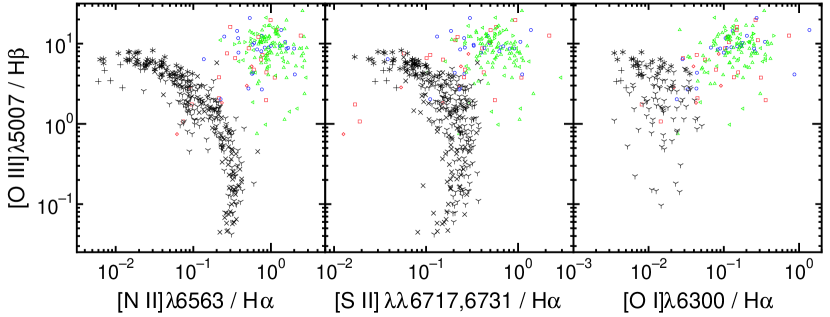
Figure 4.— Compiled objects are shown in the diagnostic diagrams proposed by Veilleux and Osterbrock (1987). The diamonds are NLS1s, the squares are BLS1s, the circles are S1.5s, the triangles pointing to the left are S2_RBLRs, those pointing to the right are S2_HBLRs, and those pointing to the upper side are S2^-. Red color means S1s, blue color means S1.5s, and green color means S2s. For comparison, compiled H ii systems are also plotted in this figure. The plus signs are blue compact galaxies (Izotov et al. 1994), the crosses and the “Y” signs are extragalactic H ii galaxies (McCall et al. 1985; van Zee et al. 1998), and the asterisks are H ii galaxies (Masegosa et al. 1994). (a) Diagram of [O iii]$\lambda$5007/H$\beta$ versus [N ii]$\lambda$6583/H$\alpha$. (b) Diagram of [O iii]$\lambda$5007/H$\beta$ versus [S ii]$\lambda\lambda$6717,6731/H$\alpha$. (c) Diagram of [O iii]$\lambda$5007/H$\beta$ versus [O i]$\lambda$6300/H$\alpha$.

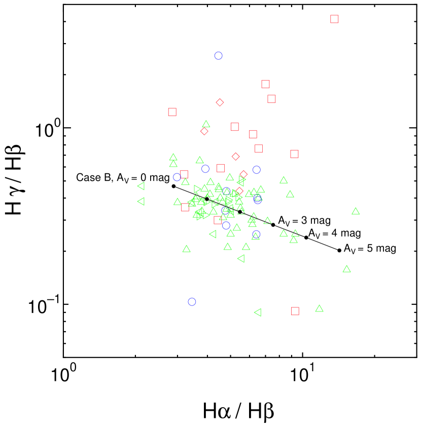
Figure 5.— Diagram of H$\gamma$/H$\beta$ versus H$\alpha$/H$\beta$. The symbols are the same as those in figure 4. Theoretically predicted emission-line ratios assuming the case B and dust extinction of 0 mag $\leq A_{V}\leq$ 5 mag are also plotted by a solid line.

Figure 6a.— Frequency distributions of the various emission-line flux ratios. (a) Flux ratio of [O i]$\lambda$6300/[O iii]$\lambda$5007. (b) Flux ratio of [O ii]$\lambda$3727/[O iii]$\lambda$5007. (c) Flux ratio of [O i]$\lambda$6300/[O ii]$\lambda$3727. (d) Flux ratio of [O iii]$\lambda$4363/[O iii]$\lambda$5007. (e) Flux ratio of [S ii]$\lambda$6717/[S ii]$\lambda$6731. (f) Flux ratio of [O i]$\lambda$6300/[S ii]$\lambda\lambda$6717,6731. (g) Flux ratio of [O ii]$\lambda$3727/[S ii]$\lambda\lambda$6717,6731. (h) Flux ratio of [S ii]$\lambda\lambda$6717,6731/[O iii]$\lambda$5007. (i) Flux ratio of [O i]$\lambda$6300/[N ii]$\lambda$6583. (j) Flux ratio of [O ii]$\lambda$3727/[N ii]$\lambda$6583. (k) Flux ratio of [N ii]$\lambda$6583/[O iii]$\lambda$5007. (l) Flux ratio of [S ii]$\lambda\lambda$6717,6731/[N ii]$\lambda$6583. (m) Flux ratio of [Ne iii]$\lambda$3869/[O iii]$\lambda$5007. (n) Flux ratio of [Ne iii]$\lambda$3869/[O ii]$\lambda$3727. (o) Flux ratio of [Ne v]$\lambda$3426/[O ii]$\lambda$3727. (p) Flux ratio of [Fe vii]$\lambda$6087/[O iii]$\lambda$5007.

Figure 6b.— continued.

Figure 6c.— continued.

Figure 6d.— continued.

Figure 6e.— continued.

Figure 6f.— continued.

Figure 6g.— continued.

Figure 6h.— continued.

Figure 6i.— continued.

Figure 6j.— continued.

Figure 6k.— continued.

Figure 6l.— continued.

Figure 6m.— continued.

Figure 6n.— continued.

Figure 6o.— continued.

Figure 6p.— continued.

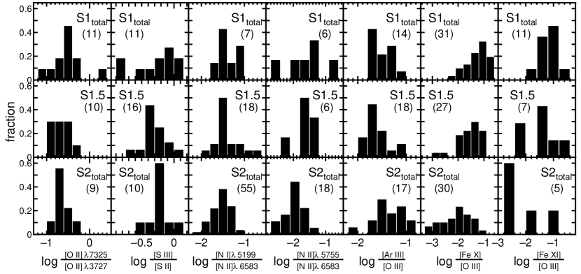
Figure 7.— Frequency distributions of the various emission-line flux ratios. Since the number of objects in each sample is small, the histograms are shown only for the S1_totals, the S1.5s, and the S2_total. (a) Flux ratio of [O ii]$\lambda$7325/[O ii]$\lambda$3727. (b) Flux ratio of [S iii]$\lambda$9069/[S ii]$\lambda\lambda$6717,6731. (c) Flux ratio of [N i]$\lambda$5199/[N ii]$\lambda$6583. (d) Flux ratio of [N ii]$\lambda$5755/[N ii]$\lambda$6583. (e) Flux ratio of [Ar iii]$\lambda$7136/[O iii]$\lambda$5007. (f) Flux ratio of [Fe x]$\lambda$6374/[O iii]$\lambda$5007. (g) Flux ratio of [Fe xi]$\lambda$7892/[O iii]$\lambda$5007.

Figure 8a.— Various emission-line flux ratios are plotted as functions of redshift, IRAS 25 $\mu$m luminosity, and IRAS 60 $\mu$m luminosity. The symbols are the same as those in figure 4. (a) Flux ratios of [O i]$\lambda$6300/[O iii]$\lambda$5007, [O ii]$\lambda$3727/[O iii]$\lambda$5007, [O i]$\lambda$6300/[O ii]$\lambda$3727, [O iii]$\lambda$4363/[O iii]$\lambda$5007 (=$R_{\rm OIII}$), [S ii]$\lambda$6717/[S ii]$\lambda$6731 (=$R_{\rm SII}$), and [O i]$\lambda$6300/[S ii]$\lambda\lambda$6717,6731. (b) Flux ratios of [O ii]$\lambda$3727/[S ii]$\lambda\lambda$6717,6731 [S ii]$\lambda\lambda$6717,6731/[O iii]$\lambda$5007, [O i]$\lambda$6300/[N ii]$\lambda$6583, [O ii]$\lambda$3727/[N ii]$\lambda$6583, [N ii]$\lambda$6583/[O iii]$\lambda$5007, and [S ii]$\lambda\lambda$6717,6731/[N ii]$\lambda$6583. (c) Flux ratios of [Ne iii]$\lambda$3869/[O iii]$\lambda$5007, [Ne iii]$\lambda$3869/[O ii]$\lambda$3727, [Ne v]$\lambda$3426/[O ii]$\lambda$3727, [Fe vii]$\lambda$6087/[O iii]$\lambda$5007, [O ii]$\lambda$7325/[O ii]$\lambda$3727 (=$R_{\rm OII}$), and [S iii]$\lambda$9069/[S ii]$\lambda\lambda$6717,6731. (d) Flux ratios of [N i]$\lambda$5199/[N ii]$\lambda$6583, [N ii]$\lambda$5755/[N ii]$\lambda$6583 (=$R_{\rm NII}$), [Ar iii]$\lambda$7136/[O iii]$\lambda$5007, [Fe x]$\lambda$6374/[O iii]$\lambda$5007, and [Fe xi]$\lambda$7892/[O iii]$\lambda$5007.

Figure 8b.— continued.

Figure 8c.— continued.

Figure 8d.— continued.

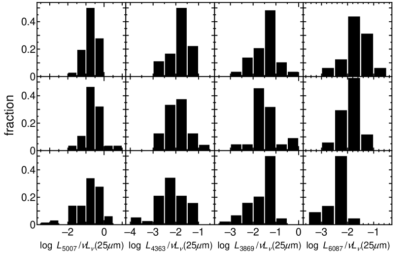
Figure 9.— Frequency distributions of the luminosities of the [O iii]$\lambda$5007 emission, the [O iii]$\lambda$4363 emission, the [Ne iii]$\lambda$3869 emission and the [Fe vii]$\lambda$6087 emission for the S1_totals, the S1.5s, and the S2_totals. These luminosities are normalized by the IRAS 25 $\mu$m luminosity.

Figure 10.— Diagram of $L$([O iii]$\lambda$5007) versus $L$([O ii]$\lambda$3727). The symbols are the same as those in figure 4.

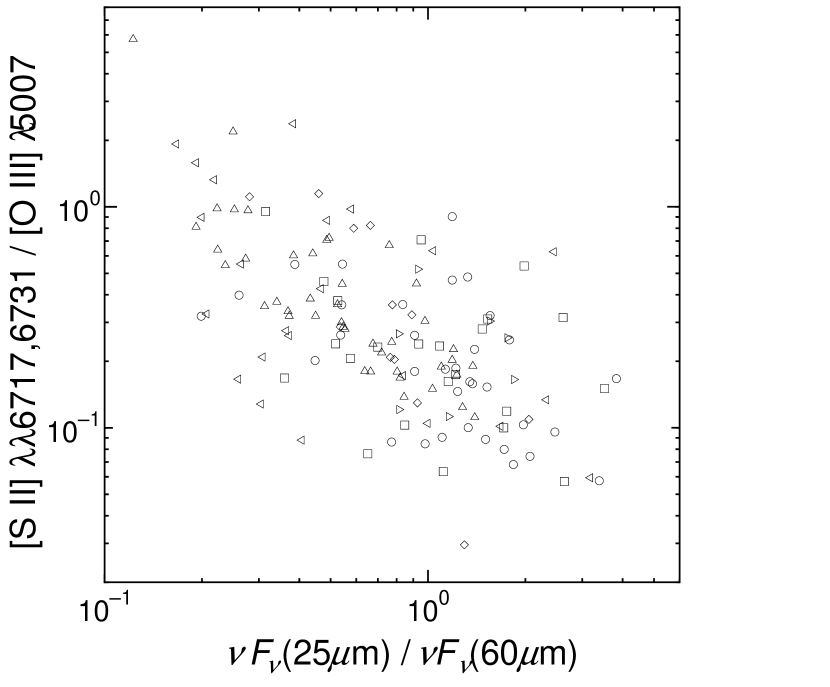
Figure 11.— Diagram of the emission-line flux ratio of [S ii]$\lambda\lambda$6717,6731/[O iii]$\lambda$5007 versus that of $\nu F_{\nu}$(25 $\mu$m)/$\nu F_{\nu}$(60 $\mu$m). The symbols are the same as those in figure 4.

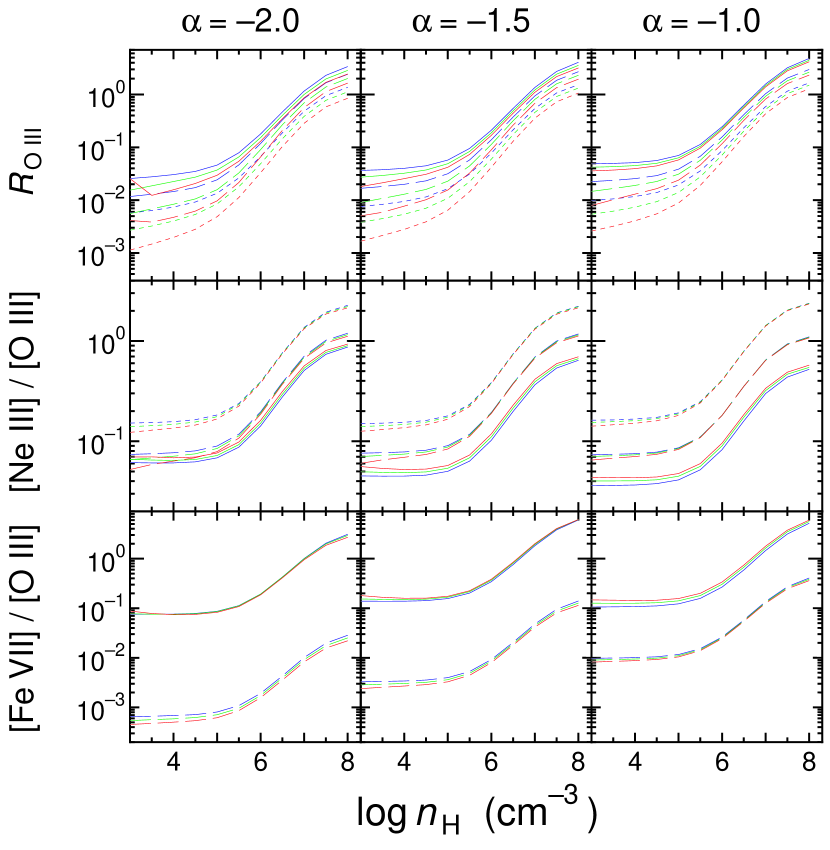
Figure 12.— Calculated emission-line flux ratios of [O iii]$\lambda$4363/[O iii]$\lambda$5007 ($R_{\rm OIII}$), [Ne iii]$\lambda$3869/[O iii]$\lambda$5007 and [Fe vii]$\lambda$6087/[O iii]$\lambda$5007 are shown as a function of the gas density. Here, the Lyman optical depth is assumed to be $\tau_{912}=0.1$. The dotted lines, the dashed lines, and the solid lines denote the models adopting $U=10^{-3.5}$, $10^{-2.5}$, and 10^-1.5, respectively. The blue lines, the green lines, and the red lines denote the models adopting the metallicity of half the solar, the solar, and twice the solar one, respectively.

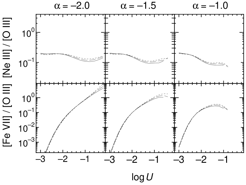
Figure 13.— Calculated emission-line flux ratios of [Ne iii]$\lambda$3869/[O iii]$\lambda$5007 and [Fe vii]$\lambda$6087/[O iii]$\lambda$5007 shown as a function of the ionization parameter. In these models, $n_{\rm H}=10^{6.0}$ cm^-3 is assumed. The solid lines denote the models with the metallicity of half the solar value, the dashed lines denote the models with the solar metallicity, and the dotted lines denote the models with the metallicities of twice the solar value.

Figure 14.— Same as figure 12, but for $\tau_{912}=0.01$. Only the models with solar metallicity are shown.

Figure 15.— Same as figure 12, but for $\tau_{912}=1.0$. Only the models with solar metallicity are shown.

References

- (1) Antonucci, R. 1993, ARA&A, 31, 473
- (2) Baker, J. C. 1997, MNRAS, 286, 23
- (3) Baker, J. C., & Hunstead, R. W. 1995, ApJ, 452, L95
- (4) Baldwin, J. A., Phillips, M. M., & Terlevich, R. 1981, PASP, 93, 5
- (5) Barth, A. J., Tran, H. D., Brotherton, M. S., Filippenko, A. V., Ho, L. C., van Breugel, W., Antonucci, R., & Goodrich, R. W. 1999, AJ, 118, 1609
- (6) Barthel, P. D. 1989, ApJ, 336, 606
- (7) Binette, L. 1985, A&A, 143, 334
- (8) Cardelli, J. A., Clayton, G. C., & Mathis, J. S. 1989, ApJ, 345, 245
- (9) Cohen, R. D. 1983, ApJ, 273, 489
- (10) Dahari, O., & De Robertis, M. M. 1988, ApJS, 67, 249
- (11) De Zotti, G., & Gaskell, C. M. 1985, A&A, 147, 1
- (12) di Serego Alighieri, S., Cimatti, A., Fosbury, R. A. E., & Hes, R. 1997, A&A, 328, 510
- (13) Efstathiou, A., & Rowan-Robinson, M. 1995, MNRAS, 273, 649
- (14) Fadda, D., Giuricin, G., Granato, G. L., & Vecchies, D. 1998, ApJ, 496, 117
- (15) Ferland, G. J. 1996, Hazy: A Brief Introduction to Cloudy (Lexington: Univ. Kentucky Dept. Phys. Astron.)
- (16) Ferland, G. J., & Netzer, H. 1983, ApJ, 264, 105
- (17) Grevesse, N., & Anders, E. 1989, in AIP Conf. Proc. 183, Cosmic Abundance of Matter, ed. C. J. Waddington (New York: AIP), 1
- (18) Grevesse, N., & Noels, A. 1993, in Origin & Evolution of the Elements, ed. N. Prantzos, E. Vangioni-Flam, & M. Cassé (Cambridge: Cambridge Univ. Press), 15
- (19) Halpern, J. P., & Steiner, J. E. 1983, ApJ, 269, L37
- (20) Heckman, T. M., & Balick, B. 1979, A&A, 79, 350
- (21) Heckman, T. M., Gonzalez-Delgado, R., Leitherer, C., Meurer, G. R., Krolik, J., Wilson, A. S., Koratkar, A., & Kinney, A. 1997, ApJ, 482, 114
- (22) Heckman, T. M., Krolik, J., Meurer, G., Calzetti, D., Kinney, A., Koratkar, A., Leitherer, C., Robert, C., & Wilson, A. 1995, ApJ, 452, 549
- (23) Hes, R., Barthel, P. D., & Fosbury, R. A. E. 1993, Nature, 362, 326
- (24) Izotov, Y. I., Thuan, T. X., & Lipovetsky, V. A. 1994, ApJ, 435, 647
- (25) Jackson, N., & Browne, I. W. A. 1990, Nature, 343, 43
- (26) Khachikian, E. Y., & Weedman, D. W. 1974, ApJ, 192, 581
- (27) Kinney, A. L., Antonucci, R. R. J., Ward, M. J., Wilson, A. S., & Wittle, M. 1991, ApJ, 377, 100
- (28) Koski, A. T. 1978, ApJ, 223, 56
- (29) Kuraszkiewicz, J., Wilkes, B. J., Czerny, B., & Mathur, S. 2000, ApJ, 542, 692
- (30) Masegosa, J., Moles, M., & Campos-Aguilar, A. 1994, ApJ, 420, 576
- (31) McCall, M. L., Rybski, P. M., & Shields, G. A. 1985, ApJS, 57, 1
- (32) Moshir, M., Kopman, G., & Conrow, T. A. O. 1992, Explanatory Supplement to the Faint Source Survey, version 2 (Pasadena: JPL)
- (33) Mulchaey, J. S., Koratkar, A., Ward, M. J., Wilson, A. S., Whittle, M., Antonucci, R. R. J., Kinney, A. L., & Hurt, T. 1994, ApJ, 436, 586
- (34) Murayama, T., & Taniguchi, Y. 1998a, ApJ, 497, L9
- (35) Murayama, T., & Taniguchi, Y. 1998b, ApJ, 503, L115
- (36) Murayama, T., Taniguchi, Y., & Iwasawa, K. 1998, AJ, 115, 460
- (37) Nagao, T. 2001, Master’s thesis, Tohoku University
- (38) Nagao, T., Murayama, T., & Taniguchi, Y. 2001a, ApJ, 546, 744
- (39) Nagao, T., Murayama, T., & Taniguchi, Y. 2001b, ApJ, 549, 155
- (40) Nagao, T., Taniguchi, Y., & Murayama, T. 2000, AJ, 119, 2605
- (41) Ohyama, Y. 1996, Master’s thesis, Tohoku University
- (42) Osterbrock, D. E. 1978, Lick Obs. Bull, No. 775
- (43) Osterbrock, D. E. 1989, Astrophysics of Gaseous Nebulae and Active Galactic Nuclei (Mill Valley: University Science Books)
- (44) Osterbrock, D. E., Koski, A. T., & Phillips, M. M. 1976, ApJ, 206, 898
- (45) Osterbrock, D. E., & Pogge, R. W. 1985, ApJ, 297, 166
- (46) Peterson, B. M. 1993,PASP, 105, 247
- (47) Pier, E. A., & Krolik, J. H. 1992, ApJ, 401, 99
- (48) Pier, E. A., & Voit, G. M. 1995, ApJ, 450, 628
- (49) Press, W. H., Teukolsky, S. A., Vetterling, W. T., & Flannery, B. P. 1988, Numerical Recipes in C (Cambridge: Cambridge University Press)
- (50) Schmitt, H. R. 1998, ApJ, 506, 647
- (51) Schmitt, H. R., & Kinney, A. L. 1996, ApJ, 463, 498
- (52) Shuder, J. M., & Osterbrock, D. E. 1981, ApJ, 250, 55
- (53) Simpson, C. 1998, MNRAS, 297, L39
- (54) Storchi-Bergmann, T., Mulchaey, J. S., & Wilson A.S. 1992, ApJ, 395, L73
- (55) Storchi-Bergmann, T., & Pastoriza, M. G. 1989, ApJ, 347, 195
- (56) Storchi-Bergmann, T., & Pastoriza, M. G. 1990, PASP, 102, 1359
- (57) Thuan, T. X. 1984, ApJ, 281, 126
- (58) van Zee, L., Salzer, J. J., Haynes, M. P., & Balonek, T. J. 1998, AJ, 116, 2805
- (59) Veilleux, S., & Osterbrock, D. E. 1987, ApJS, 63, 295 (VO87)
- (60) Véron-Cetty, M. -P., & Véron, P. 2000, ESO Sci. Rept. 19 (European Southern Observatory)
- (61) Wilkes, B. J., Schmidt, G. D., Smith, P. S., Mathur, S., & McLeod, K. K. 1995, ApJ, 455, L13
- (62)