The distribution of mass around galaxies

Abstract

We explore the distribution of mass about the expected sites of galaxy formation in a high-resolution hydrodynamical simulation of a $\Lambda$CDM cosmology which includes cooling, star-formation and feedback. We show that the evolution of the galaxy bias is non-trivial and non-monotonic and that the bias is stochastic. We discuss the galaxy-mass cross-correlation function and highlight problems with the interpretation of galaxy-galaxy lensing as due to extended dark matter halos around “typical” galaxies. Finally we show that the “external shear” around strong gravitational lenses is likely to be closely aligned with the direction of the nearest massive galaxy and to have a power-law distribution which can be predicted from the galaxy auto-correlation function.

1. Introduction

The distribution of galaxies with respect to the total mass in the Universe remains a central unsolved problem in cosmology, though one which is becoming increasingly amenable to theoretical modeling and ever more constrained observationally. In particular, gravitational lensing allows us to probe the spatial distribution of the mass in the Universe, for example around galaxies and in clusters of galaxies. In this paper we present predictions for the distribution of mass around sites of galaxy formation using a hydrodynamic simulation of structure formation which includes cooling, star-formation and feedback. We believe such simulations can provide ab initio and robust predictions for the statistical distribution of the sites of galaxy formation, even though the detailed star formation rates and galaxy morphologies are sensitive to uncertain “sub-resolution” physics. As such, these simulations can be used to predict, from first principles, the galaxy auto-correlation function, the galaxy-mass cross correlation function (which is the key ingredient in galaxy-galaxy lensing studies) and the mass auto-correlation function.

Originally regarded as an interesting, but not practically useful, prediction of Einstein’s theory of general relativity, gravitational lensing has become a “standard” tool in observational cosmology. Strong gravitational lensing has a long history, and weak lensing of background galaxies by clusters of galaxies is now well established. Just recently the weak lensing of galaxies by large-scale structure has been observationally demonstrated (van Waerbeke et al. Ludo (2000); Bacon et al. BRE (2000); Kaiser et al. KWL (2000); Wittman et al. WTKDB (2000); Maoli et al. Maoli (2001); Rhodes et al. RRG (2001)), at about the level predicted by theories based on gravitational instability in a cold dark matter (CDM) dominated universe.

The weak lensing observations probe the (projected) distribution of mass in the Universe directly, without reference to the distribution of light. This provides us with direct constraints on the dark matter auto-correlation function, for which theoretical predictions are very well developed both analytically and numerically on Mpc scales. By contrast, galaxy redshift surveys can give us detailed three-dimensional information about the distribution of luminous matter, providing us with a measure of the galaxy auto-correlation function and its evolution. However, galaxy formation is still poorly understood, making interpretation of the full information contained in the galaxy auto-correlation function difficult.

Intermediate between these two are dark matter-galaxy cross-correlations. These can be measured whenever the galaxy distribution is cross-correlated with a tracer of the dark matter. Some examples are galaxy-galaxy lensing (correlating galaxies and weak lensing shear), foreground-background galaxy correlations and galaxy-QSO correlations (correlating galaxies with weak lensing magnification). All of these can be interpreted as a projection of the galaxy-mass correlation function which we shall discuss. To understand the galaxy-mass cross-correlation requires us to understand the environments of galaxies, but not necessarily the detailed properties of the galaxies themselves.

Another probe of the mass distribution around galaxies comes from strong gravitational lensing. Although the central regions of the primary lens galaxy, whose spatial structure is not well modeled by current calculations, dominates the monopole gravity in a strong lens, the quadrupole (and to a lesser extent the higher poles) has a significant contribution from the external shear or tidal gravity near the lens or along the line-of-sight. All lensing models require this degree of freedom (Barkana Barkana96 (1996); Keeton, Kochanek & Seljak Keeton97 (1997)) and in some cases the dominant source can be clearly identified with a nearby galaxy.

The outline of this paper is as follows: we review the simulation we shall use in §2, giving details of how we identify galaxies and their parent halos. The evolution of clustering in the simulation is discussed in §3 and we introduce our primary tool, the correlation function in §4. The implications of our simulation for the interpretation of galaxy-galaxy lensing is dealt with in §5. Models of external shear for strong lensing are dealt with in §6. Finally in §7 we summarize our findings.

2. The simulation

Throughout, we shall use a new simulation of the Ostriker & Steinhardt (OstSte (1995)) concordance model, which has $\Omega_{\rm m}=0.3$, $\Omega_{\Lambda}=0.7$, $H_{0}=100\,h\,{\rm km}{\rm s}^{-1}{\rm Mpc}^{-1}$ with $h=0.67$, $\Omega_{\rm B}=0.04$, $n=1$ and $\sigma_{8}=0.9$ (corresponding to $\delta_{H}=5.02\times 10^{-5}$). This model yields a reasonable fit to the current suite of cosmological constraints and as such provides a good framework for making realistic predictions.

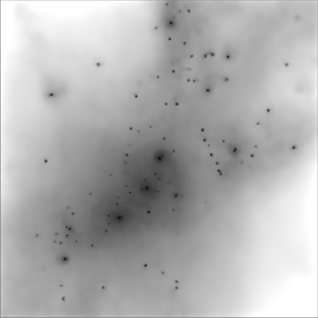
Figure 1.— The projected mass density in the vicinity of the largest group in the simulation at $z=0.7$. The grey scale indicates the projected gas density (in $h^{-1}M_{\odot}/(h^{-1}{\rm Mpc})^{2}$) within a cube of side $3h^{-1}$Mpc centered on the most bound particle in the group. Small knots of dense gas, which we identify as sites of galaxy formation, can be seen clearly. Like many large groups, this one is part of a large filamentary structure, which explains the spatial orientation of the distribution of sub-halos.

We have used the Tree/SPH code Gadget (Springel, Yoshida & White SprYosWhi (2001)) to run a $2\times 300^{3}=54$ million particle simulation of this model in a periodic box of size $33.5\,h^{-1}$Mpc. Equal numbers of gas and dark matter particles were employed, so $m_{\rm dark}=1.0\times 10^{8}\,h^{-1}M_{\odot}$ and $m_{\rm gas}=1.5\times 10^{7}\,h^{-1}M_{\odot}$. The gravitational interaction between particles is softened on small scales using a cubic spline (e.g. Hernquist & Katz HerKatz (1989)) and the ‘Plummer equivalent’ gravitational softening in our simulation was $6\,h^{-1}$kpc, fixed in comoving coordinates. The simulation was started at redshift $z=99$ and evolved to $z=0$. Unfortunately the simulation box is too small to reliably predict clustering properties at very low redshifts, as the fundamental mode becomes increasingly non-linear for $z<1$. Hence, in this paper we restrict our analysis to redshifts $z\geq 0.5$.

In addition to the gravitational interactions and adiabatic hydrodynamics, the code follows radiative cooling and heating processes in the presence of a UV radiation field in essentially the same way as described in Katz, Weinberg & Hernquist (KatWeiHer (1996)). We model the UV radiation field using a modified Haardt & Madau (HaaMad (1996)) spectrum with reionization occuring at $z\approx 6$ (see e.g. Davé et al. 1999), and with an amplitude chosen to reproduce the mean opacity of the Lyman-alpha forest at $z=3$ (e.g. Rauch et al. 1997). Star formation (and feedback) is handled using a modification of the “multi-phase” model of Yepes et al. (YepKatKhoKly (1997)) and Hultman & Pharasyn (HulPha (1999)). Each SPH particle is assumed to describe a co-spatial fluid of ambient hot gas, condensed cold clouds, and stars. Hydrodynamics is followed for only the hot gas phase, but the cold gas and stars are subject to gravity, add inertia, and participate in mass and energy exchange processes with the ambient gas phase. The algorithm will be described in more detail in a forthcoming paper.

From the simulation outputs we have constructed catalogues of halos and their sub-halos using the algorithm Subfind described in detail in Springel et al. (SWTK (2000)). First, the Friends-of-Friends algorithm (with a linking length of $0.15\bar{n}^{-1/3}$) is used to define a parent halo catalogue, and then bound sub-halos within each parent are identified. Sub-halos are defined as locally overdense, gravitationally bound structures. These sub-halos typically consist of cold, dense gas at their center, surrounded by a halo of dark matter and tenuous hot gas. The halo may be severely truncated if the sub-halo is not the central galaxy in the parent halo, but the dense gas that has been able to efficiently cool and form stars should allow a reliable identification with galaxies in the real Universe, at least statistically (see Fig. 1).

$z$	$N_{\rm sub-halo}$	$N(>M_{\rm sub})$	$N(>M_{\rm fof})$	$f_{\rm iso}$
3.00	39579	7066	9742	73%
2.00	39248	9478	13339	71%
1.75	38233	9802	13752	71%
1.50	36959	10129	14158	70%
1.25	35819	10294	14489	71%
1.00	34422	10333	14514	70%
0.70	33143	10165	14583	70%
0.50	32234	9958	14512	70%

Table 1The number of sub-halos found in the simulation as a function of redshift. The first column is the total number of sub-halos with more than 32 particles. The second column is the number of sub-halos with $M_{500}>10^{10}\,h^{-1}M_{\odot}$. Third, the number of sub-halos which live in a parent “FOF” halo with $M_{500}>10^{10}\,h^{-1}M_{\odot}$. The last column lists the fraction of sub-halos above $10^{10}\,h^{-1}M_{\odot}$ which are “isolated”, i.e. are the only members of their parent halo.

We have used a linking length of 0.15 rather than the more canonical 0.2 in defining the parent halos, because we found for the larger linking length two neighboring but distinct halos were frequently linked into one parent halo, with one of them then identified as a sub-halo of the other. While this problem is not eliminated entirely using a linking length of 0.15, it is significantly reduced. Only very close halo pairs or triplets, possibly in the process of merging, are joined with this linking length. In some instances the FOF algorithm finds halos which are not bound; these halos have in general very small particle number and are not included in the analysis. Results from the halo finding are shown in Table 1.

For each halo or sub-halo we define the “center” as the position of the particle with the minimum potential energy, with the potential calculated using only the group particles. This definition usually corresponds very closely to the most bound and densest particles, and is more robust than the center of mass. Many definitions of mass are possible and can differ from each other quite significantly (e.g. White HaloMass (2001)). Although counting the particles within the FOF group is the simplest, we have chosen to follow a more commonly used approach where the mass is defined as that enclosed within a radius inside of which the mean density is 500 times the critical density. An alternative definition could use the background density rather than the critical density. The two scale differently with redshift except for cosmologies with critical matter density. At the redshifts at which we are working the density contrast with respect to background scales as $\left[\Omega_{\rm m}+\Omega_{\Lambda}(1+z)^{-3}\right]$.

	$\log_{10}(M_{500}/M_{\odot})$
$z$	10-11	11-12
3.00	76%	27%
2.00	76%	16%
1.75	76%	19%
1.50	76%	17%
1.25	77%	18%
1.00	77%	19%
0.70	77%	17%
0.50	77%	19%

Table 2Fraction of sub-halos which are isolated as a function of mass and redshift. There are no halos in the simulation with $M_{500}>10^{12}\,h^{-1}M_{\odot}$ which are isolated for $z\geq 0.5$!

In Fig. 2 we show a scatter plot of the masses of the sub-halos and their parent halos at $z=1$. Most of the halos are isolated and have parent halo masses fractionally larger than the sub-halo masses. As the parent halos become more massive there is less chance that it hosts only one galaxy. In our first pass through we found that there are a very small number of systems where the sub-halo mass exceeds the parent halo mass. This can arise in situations where several halos are merging, with the bridging material being at low density. If the most bound particle in the group lies at the center of a less massive sub-halo our definition of mass, $M_{500}$, returns the mass of this sub-halo as the “parent” mass. In such cases we replace the “parent” mass with the sum of the sub-halo masses to more accurately reflect the total mass of the system.

$z$	$\langle z_{\rm form}\rangle$
3.00	4.8
2.00	3.3
1.75	3.0
1.50	2.7
1.25	2.4
1.00	2.2
0.90	2.1
0.80	2.0
0.70	1.9
0.60	1.8
0.50	1.7

Table 3The (mass weighted) mean redshift of star formation as a function of redshift.

Figure 2.— A scatter plot of $M_{500}$ for the sub-halos and their parent FOF halos from the simulation at $z=1$.

Ideally, we would identify the sub-halos as galaxies by some observational property, such as luminosity or color. Unfortunately, it is difficult to reliably compute such properties from this simulation, because the outputs are too infrequent to graft on population synthesis codes. However we do give, in addition to the total mass of a sub-halo, results as a function of the stellar mass within $r_{500}$ of the sub-halo center. We do this under the assumption that the near infrared magnitude of a galaxy should roughly track its stellar mass (e.g. Cole et al. 2dF-Kband (2001)). The (mass weighted) mean age of the stars at each output is given in Table 3 to help with this conversion. Finally, to help in matching our halos to observed galaxies we give the number density of our halos, as a function of $z$, in Fig. 3. As a first approximation, and in the absence of further information, one can match halos of a given mass to objects of an equivalent space density.

Figure 3.— The mass function for the simulation at $z=2$ (top), 1 (middle) and $0.5$ (bottom). Solid symbols are for the “parent” halos found with FOF with a linking length of 0.15. Open symbols count halos identified by the sub-halo finder, removing unbound particles. We show the mass function as a function of total mass (squares), gas mass (circles) and stellar mass (triangles). In all cases the mass quoted is $M_{500}$ in $h^{-1}\,M_{\odot}$ (see text).

3. The clustering of sub-halos

We are interested in the clustering of galaxies and dark matter, and its evolution with time, within this simulation. We show in Fig. 4 the dark matter power spectra at $z=4$, 3, 2 and 1. To compute these power spectra we estimated the dark matter density field from the particles using NGP assignment (Hockney & Eastwood HocEas (1988)) onto a $256^{3}$ grid. The density field was then Fourier Transformed to obtain $\delta_{k}$. The power spectrum was obtained by binning $\left|\delta_{k}\right|^{2}$ in shells in $\vec{k}$-space, corrected for the binning, the mass assignment onto the grid and shot-noise (see e.g. Peacock & Dodds PD96 (1996) for a discussion of some of these issues). To extend the calculation to higher $k$ we repeated the process several times, rescaling the particle separations by increasing factors and remapping the distribution into the periodic volume each time (Peacock, private communication; Jenkins et al. Jen98 (1998)). This provides us with an estimate of $P(k)$ limited only by the resolution of the simulation, and not by the size of the Fourier transform grid.

Compared to semi-analytic estimates of the expected power (Peacock & Dodds PD96 (1996)) we find that this box has a slight shortfall. To check whether the semi-analytic model correctly estimates the dark matter power spectrum for this model we have run two additional dark matter only simulations, each using $256^{3}$ particles. The first simulation is in a $200h^{-1}$Mpc box and the second in a $100h^{-1}$Mpc box. The power spectra computed from the $z=1$ outputs of these runs in the same manner as above are also shown in Fig. 4. We see that the fitting function has slightly less power than the simulation at small scales, as seen also in the simulations of Jain, Mo & White (JaiMoWhi (1995)). The power spectrum in our $33.5h^{-1}$Mpc box is low on all scales at the redshifts of interest, although the shape is approximately correct. Fluctuations in the amplitude, but not the shape, of the power spectrum due to finite volume effects are well known (e.g. Meiksin & White MeiWhi (1999)). Part of the shortfall in power is due to the particular random phases chosen in the initial conditions, the remainder is due to the fact that the box is becoming less and less of a fair sample of the Universe as time evolves and the non-linear scale increases. We show the latter effect by plotting, in Fig. 5, the growth of the fundamental mode, $\Delta^{2}(k_{f})$, compared with linear theory. As long as the box remains a fair sample of the Universe the ratio $\Delta^{2}(k_{f})/D^{2}(z)$, where $D(z)$ is the linear growth factor, should remain constant.

Figure 4.— The dimensionless dark matter power spectrum as a function of redshift. The solid lines indicate the expected non-linear power spectrum for this model, as estimated using the formalism of Peacock & Dodds (PD96 (1996)) at $z=1$, 2, 3 and 4 (top to bottom). The solid symbols are the power spectra at $z=1$ from two $256^{3}$ DM only simulations in boxes of size $200h^{-1}$Mpc (squares) and $100h^{-1}$Mpc (triangles) which provide and estimates of the uncertainty in the Peacock & Dodds formalism. The open circles indicate the power spectra from the simulation in this work, the $33.5h^{-1}$Mpc hydro simulation, at $z=1$, 2, 3 and 4 (top to bottom).

In earlier work (White et al. WhiHerSpr (2001)) we showed that the number of “galaxies” per dark matter halo scaled approximately as a power-law in the parent halo mass with an index less than 1 (typically 0.7-0.8). This behavior is precisely what is needed to explain the observed clustering of galaxies (e.g. Scoccimarro et al. SSHJ (2000)) and is also seen in semi-analytic models (e.g. Seljak Sel (2000)). The spatial distribution of sub-halos in the simulation is consistent with the assumption that every halo hosts a galaxy which resides at its center and any extra satellite galaxies trace the dark matter distribution. It remains an open question observationally whether the galaxy density traces the mass density in halos (e.g. Adami et al. AMUS (2001)).

Figure 5.— The power in the fundamental mode vs linear theory. We plot the ratio of $\Delta^{2}(k_{f})$ to the linear growth factor, $D(z)$. This should be constant as long as the box is a fair sample of the Universe. The power begins to fall below the linear theory prediction at late times because our periodic box is missing long-wavelength power on scales larger than the fundamental mode, which are not available to be coupled into the evolution as $k_{f}$ goes non-linear.

We performed a counts-in-cells analysis of both the mass and galaxy number density fields as a function of redshift. First, we divided the cubical box up into a grid of cells with $N_{c}=32$, 64, 128 or 256 cells on a side. We assigned each particle or galaxy to the appropriate cubical cell weighting the particles by their mass and the galaxies equally. For the galaxies, we treated them as points at the position of their potential minima. This was done 8 times with the grid shifted to a random position each time. Then, we calculated the variance of mass and galaxy fluctuations, from which we can define $b\equiv\sigma_{\rm gg}/\sigma_{\rm mm}$, the covariance $b^{\prime}\equiv\sigma^{2}_{\rm gm}/\sigma_{\rm mm}^{2}$ and the cross-correlation coefficient $r\equiv\sigma^{2}_{\rm gm}/\sigma_{\rm gg}\sigma_{\rm mm}$. Our results are shown in Table 4. We see a clear tendency for the bias to be “stochastic”, with decreasing correlation between the galaxies and the total mass as we probe smaller length scales.

$N_{c}$	$\sigma_{\rm mm}$	$\sigma_{\rm gg}$	$r$
16	1.87	1.59	0.83
32	3.56	3.02	0.73
64	6.59	6.45	0.61
128	11.2	15.7	0.51
256	18.0	41.6	0.46

Table 4Counts-in-cells of the mass and galaxy number density fields at $z=1$. The first column is the number of cells in each dimension of the box, the second column gives the rms fluctuation in the mass (in units of the mean), the third the rms fluctuation in the galaxy number density (using only galaxies with $M_{500}>10^{10}\,h^{-1}M_{\odot}$) and the final column gives the cross correlation coefficient. We have stopped at $N_{c}=256$ since to implement finer grids we would need to use the extent of the sub-halos rather than just their positions.

4. Correlation function

We identify the center of a “galaxy” as the position of the minimum of the potential of a bound sub-halo found with Subfind. Around each such center we calculate the probability, in excess of random, of having mass $M$ within a spherical shell of radius $r$ and width $dr$. Stellar mass, cold and hot gas mass and dark matter are all included in this accounting. We present our results in terms of the correlation function which we define as

$$\xi_{\rm gm}\equiv{M(r;dr)\over\langle M(r;dr)\rangle}-1,$$ (1)

where $M(r;dr)$ is the mass contained within the shell between radius $r$ and $r+dr$ and $\langle\cdots\rangle$ indicates an average quantity. To safely avoid numerical resolution effects we shall consider galaxies only above $10^{10}\,h^{-1}M_{\odot}$.

We show in Fig. 6 the correlation function of the mass, $\xi_{\rm mm}(r)$, the galaxies above $10^{10}h^{-1}M_{\odot}$, $\xi_{\rm gg}(r)$, and the galaxy-mass cross correlation, $\xi_{\rm gm}(r)$, at $z=1$, 2 and 3. The correlation functions are well described by power laws (with a slowly changing slope) and on scales above a few$\times 100h^{-1}$kpc the galaxy-mass cross correlation function is just the geometric mean of the mass-mass and galaxy-galaxy autocorrelation functions (see Fig. 7). While the mass correlation function grows steadily with time the evolution of the galaxy correlation function is more complicated. We give the correlation length, $r_{0}$, defined as $\xi(r_{0})=1$, vs. redshift in Table 5. Note that on length scales approaching $1h^{-1}$Mpc our box is missing power (as described above) and so these correlation lengths are biased low. These results are broadly consistent with the clustering properties of “galaxies” in simulations reported by Katz et al. (KHW92 (1992, 1999)) once differences in mass resolution, box size and galaxy identification are taken into account.

Finally, we make a distinction between two types of galaxies, those that are the sole resident of a dark matter halo (“isolated galaxies”) and those which are members of a larger halo containing several sub-halos (see Tables 1, 2). As expected the more massive galaxies reside in the more massive parent halos which host more than one sub-halo and so the isolated fraction decreases with mass. Most of the lower mass sub-halos are isolated. As we shall see below, we expect the traditional interpretation of galaxy-galaxy lensing to be more correct for the isolated galaxies, which in our case means those of low mass.

Figure 6.— The 2-point correlation functions of the mass (solid lines), galaxies with $M_{500}>10^{10}h^{-1}M_{\odot}$ (dashed) and the galaxy-mass cross correlation function (dotted) at $z=1$, 2 and 3.

Figure 7.— The cross correlation coefficient for the parameters in Fig. 6. The signal is noisy for high redshift and small distance, due to the finite number of “galaxies” and mass resolution limitations in the simulation.

	$r_{0}$
$z$	fit	mm	gm	gg
3.00	900	765	1130	1700
2.00	1500	1200	1350	1600
1.75	1750	1300	1400	1600
1.50	2000	1400	1500	1600
1.25	2400	1600	1600	1650
1.00	2800	1800	1700	1700
0.70	3350	2200	2000	1900
0.50	3800	2550	2300	2000

Table 5The correlation length $r_{0}$ defined by, $\xi(r_{0})=1$, in $h^{-1}$kpc, as a function of redshift. The first column (fit) gives the dark matter auto-correlation length computed from the fitting function of Peacock & Dodds (PD96 (1996)), the other three columns give the lengths computed from the simulation. Note the shortfall in power, discussed in the text. The mass correlation function $\xi_{\rm mm}$ increases monotonically with time while the galaxy auto-correlation function (for galaxies with $M_{500}>10^{10}h^{-1}M_{\odot}$), $\xi_{\rm gg}$, and galaxy-mass cross-correlation, $\xi_{\rm gm}$, show more complicated evolution.

5. Galaxy-galaxy lensing

Figure 8.— The spherically averaged mass profile, scaled to the background density $\bar{\rho}=\Omega_{\rm m}\rho_{\rm crit}$, for the 4 “galaxies” with $M_{500}$ within 5% of $10^{12}h^{-1}M_{\odot}$, extracted from the $z=1$ output. The solid lines include all of the mass, the dotted lines only the baryonic (gas$+$stellar) mass. The dashed lines show NFW profiles with $c=5$ and 10 (see Eq. 2). The secondary “peaks” in the profiles are due to neighboring halos – as discussed in the text none of these “galaxies” are isolated though all are centrally located in the parent halo.

The observational study of galaxy-galaxy lensing has a long history (Tyson et al. TVJM (1984)) although only recently have definitive detections been made by several groups (Brainerd et al. BraBlaSma (1996); Dell’Antonio & Tyson DelTys (1996); Griffiths et al. GCIR (1996); Hudson et al. HGDK (1998); Natarajan et al. NKSE (1998); Wilson et al. WKLC (2000); Fischer et al. SDSS (2000)). Such studies have traditionally been interpreted as constraints on extended dark matter halos around “typical” galaxies (see Fig. 8). A more modern interpretation, within the context of large-scale structure, is as a projection of the 3D galaxy-mass correlation function (Kaiser Kai92 (1992)). As with any such projection, the effect of material along the line-of-sight but not physically associated with the object in question can be a serious one (see e.g. Metzler, White & Loken MetWhiLok (2001)). We shall not address this issue here, focusing instead on the underlying 3D correlation function itself and its interpretation.

Similar work on galaxy-galaxy lensing has already been presented by Guzik & Seljak (GuzSel (2000)) using semi-analytic models of galaxy formation. By comparison with the semi-analytic models, our simulations have better spatial and mass resolution and include far more physics. Unfortunately limitations on computer resources have forced us to simulate a relatively small volume of space. This both reduces the size of our samples for statistical purposes and limits the minimum redshift to which we can accurately follow the development of large-scale structure. It is thus encouraging that our results are in good agreement with theirs in many respects.

Figure 9.— (top) The profile obtained from the simulation at $z=0.5$ if we interpret $\xi_{\rm gm}(r)$ as a density profile through $\rho_{\rm eff}(r)\equiv\bar{\rho}\left(1+\xi_{\rm gm}(r)\right)$. The bold curve indicates the region where we have explcitly computed $\xi_{\rm gm}$ from the simulation, the rest is power-law extrapolation. The dashed lines are NFW profiles with $M_{\rm vir}=2\times 10^{11}\,h^{-1}M_{\odot}$ and $c=5$ and 10 (see text). (bottom) The rotation curve from this profile, assuming $v_{c}=\sqrt{GM/r}$, and for the two NFW profiles.

As a first step we therefore ask how $\xi_{\rm gm}(r)$ relates to the profile of an “average” galaxy in our simulation? As shown in Fig. 8, the spherically averaged profiles of our halos are reasonably well fit by the NFW profile (Navarro et al. NFW (1996)):

$$\rho(r)={\rho_{0}\over x(1+x)^{2}}\qquad,$$ (2)

where $x=r/r_{s}$ is the radius scaled in units of a characteristic radius $r_{s}$. The central density is fixed by specifying the halo mass. While we have worked throughout in terms of $M_{500}$, the mass of the halo is typically defined to be the virial mass $M=(4\pi/3)\delta_{\rm vir}\rho_{\rm crit}r_{\rm vir}^{3}$ where we take the virial radius, $r_{\rm vir}$, as the radius within which the mean density enclosed is $\delta_{\rm vir}$ times the critical density. Since our cosmology has $\Omega_{\rm m}\neq 1$, the top-hat model prediction for $\delta_{\rm vir}$ is redshift dependent, taking the value $\delta_{\rm vir}\simeq 100$ at $z=0$, $\delta_{\rm vir}\simeq 140$ at $z=0.5$ and $\delta_{\rm vir}\to 18\pi^{2}$ as $z\to\infty$. The parameter $c\equiv r_{\rm vir}/r_{s}$ measures the degree of central concentration of this mass.

To estimate a profile from the cross correlation we define $\rho_{\rm eff}(r)\equiv\bar{\rho}\left(1+\xi_{\rm gm}(r)\right)$, using a power-law extrapolation to extend the range for both large and small radius beyond what we have computed explicitly from the simulation. The results are shown in Fig. 9 along with two NFW profiles of virial mass $M_{140}=1.8\times 10^{11}\,h^{-1}M_{\odot}$, which is the “average” mass of halos in the simulation at $z=0.5$.

The concept of an “average” mass is somewhat nebulous. Simply averaging $M_{500}$ for the halos identified at $z=0.5$ gives $\langle M_{500}\rangle=9\times 10^{10}h^{-1}M_{\odot}$. Relating this to a virial mass is complicated by the fact that the concentration, $c$, and thus the ration $M_{\rm vir}/M_{500}$, varies with mass. An alternative route is to use the Jenkins et al. (JFWCCEY (2000)) fit to the mass function to compute

$$\langle M\rangle\equiv{\int_{M_{\rm cut}}^{\infty}Mdn\over\int_{M_{\rm cut}}^{\infty}\ dn}$$ (3)

above $M_{\rm cut}=1.4\times 10^{10}\,h^{-1}M_{\odot}$. The limiting mass is obtained by converting $M_{500}=10^{10}\,h^{-1}M_{\odot}$ to $M_{140}$ for an NFW profile with $c=10$. [We find that for $z>0.5$ the virial mass and $M_{200}$ differ by less than 10%, so one could alternatively use $M_{200}$ throughout.] We employ this conversion because the virial mass is closer to the “mass” definition used by Jenkins et al. (JFWCCEY (2000)) than the $M_{500}$ values preferred in this study. While several steps are involved here, White (HaloMass (2001)) has shown that using an NFW profile to convert between such mass definitions works very well. Varying the value of the concentration parameter in our conversion from $M_{500}$ to $M_{140}$ makes little difference to our average mass. For a concentration of $5$ the mass ratio is $M_{140}=1.6M_{500}$ and $M_{\rm cut}=2\times 10^{11}\,h^{-1}M_{\odot}$.

As we can see the NFW profiles, while providing a good fit to individual “galaxies” within the simulation (e.g. Fig. 8) do not provide a very good fit to the profile $\rho_{\rm eff}(r)$. Also, using $\rho_{\rm eff}(r)$ we would estimate that the virial mass of an “average” galaxy is $M_{102}=1.0\times 10^{11}\,h^{-1}M_{\odot}$ ($M_{500}=5.2\times 10^{10}\,h^{-1}M_{\odot}$, c.f. $9\times 10^{10}$ above), a factor of two lower than the average computed above. Finally we note that the associated rotation curve for our “average” galaxy is much flatter than the rotation curves for the individual galaxies making up the average. This is a consequence of the varying virial radii and the weighting by the mass function and is not reflecting the distribution of matter in the individual halos.

These results suggest that galaxy-galaxy lensing, wherein one increases the signal-to-noise by stacking many galaxies, is not in fact measuring the profile of an “average” galaxy in the usual sense of these words. The main problem is that galaxies come in a wide range of masses and sizes, and live in a range of environments so the naive averaging loses its significance. If it were possible to restrict the galaxies going into the average then a more faithful representation could be obtained (although projection effects could still be a significant source of error), but we have no a priori way of knowing the galaxy mass. These issues should be borne in mind when attempting to use a weak lensing analysis to estimate halo profiles or mass-to-light ratios from galaxy-galaxy lensing.

There are two effects which muddy the waters. First, not all galaxies are the sole members of their dark matter halos. Even for those galaxies which are “isolated” what one measures is the integral over the mass function of halo profiles. Since more massive halos are in general larger, there is no sense in which one measures an “average” profile. For example, Seljak (Sel (2000)) has suggested that much of the large-$r$ signal in this case comes from the larger halos rather than the asymptotic behavior of the smaller halos.

Figure 10.— The galaxy-mass cross correlation, $\xi_{\rm gm}(r)$ at $z=1$. In each panel the solid line is the cross correlation including all massive galaxies. In the top panel, we show separately the contributions from “isolated” galaxies (dotted lines) and from galaxies sharing halos (dashed lines). In the middle panel we show the cross correlation around galaxies with total masses $10^{10}h^{-1}\,M_{\odot}\leq M_{500}<10^{11}h^{-1}\,M_{\odot}$ (dotted), $10^{11}h^{-1}\,M_{\odot}\leq M_{500}<10^{12}h^{-1}\,M_{\odot}$ (short dashed), $10^{12}h^{-1}\,M_{\odot}\leq M_{500}<10^{13}h^{-1}\,M_{\odot}$ (long dashed). The more massive sub-halos are rare, leading to a noiser signal. In the lower panel we show the cross correlation around galaxies with stellar masses $10^{9}h^{-1}\,M_{\odot}\leq M_{500}<10^{10}h^{-1}\,M_{\odot}$ (dotted), $10^{10}h^{-1}\,M_{\odot}\leq M_{500}<10^{11}h^{-1}\,M_{\odot}$ (short dashed), $10^{11}h^{-1}\,M_{\odot}\leq M_{500}<10^{12}h^{-1}\,M_{\odot}$ (long dashed). The situation at higher and lower redshifts is very similar to that shown here.

In Fig. 10 we show that, although the “isolated” galaxies are the majority of the number counts (Table 1, see also White et al. WhiHerSpr (2001)), the signal for $\xi_{\rm gm}(r)$ is intermediate between that for isolated and non-isolated groups. The two curves begin to merge at very large radius where the density is becoming close to the cosmic mean. This suggests that at larger radius ($r\sim 1h^{-1}$Mpc) we are probing not the galactic mass profile but the general distribution of matter and the isolated and non-isolated galaxies have similar large-$r$ profiles. Further,the fact that $\xi_{\rm gm}$ differs from the isolated halo case at smaller $r$ indicates that even there one is not measuring the profile of the galactic halo. Galaxies which are part embedded in larger halos contribute disproportionately to the signal from $10h^{-1}$kpc out to several $100h^{-1}$kpc. It is this “intermediate” range of radii where the signal is dominated by larger halos, as Seljak (Sel (2000)) suggests. In either case, when one measures $\xi_{\rm gm}(r)$ one is not simply measuring the mass profile around a galaxy located at the center of its dark matter halo.

Guzik & Seljak (GuzSel (2000)) have suggested that isolated galaxies should show stronger cross-correlation at small-$r$ and fixed mass, since they are all centrally located within their halos. At fixed galaxy (i.e. sub-halo) mass the opposite effect is true, since the non-isolated galaxies tend to live in more massive halos. However, if we hold the mass of the parent halo rather than that of the galaxy fixed we can correct for this effect. We find that if we do this then the central galaxies are often in denser environments, in the sense that $\xi_{\rm gm}$ is larger at very small $r\sim 10\,h^{-1}$kpc. However by $r\sim 100\,h^{-1}$kpc the opposite effect is true and the non-isolated galaxies have the stronger cross correlation. This persists until $r\sim 1\,h^{-1}$Mpc where the cross correlations for isolated and non-isolated galaxies are equal. We also note that the density around the peak is determined primarily by the mass and formation time of the sub-halo, not on whether it is part of a larger structure. Second, many of our systems contain distinct sub-halos, in which however the “bridging” material is at quite high density (indicating that it really is part of a larger structure and not an artifact of our group finding technique). In some sense all of these sub-halos are “central” and have a similar mass profile even though they belong to a larger halo. This shows that the idealization of spherical parent halos is a poor approximation to the groups we see in the simulation.

To understand the effect of the integration over mass we show the signal broken up in different ways in Fig. 10. In the middle panel of Fig. 10 we break things down by the mass of the galaxy itself. Since there is a trend for more massive galaxies to be larger and to live in more massive parent halos, their cross-correlation is larger. Again, even though the vast majority of galaxies (by number) have low mass, the signal comes from a range of masses. We also break the signal down by the galaxy stellar mass, under the assumption that the stellar mass is roughly tracing the near infrared luminosity of a galaxy and the trends are similar to the total mass case.

Thus it appears that the oft-stated claim that galaxy-galaxy lensing probes the profile of dark matter halos around galaxies is not true in detail.

6. Strong lensing and external shear

The angular structure in the gravitational field near a multiple-image gravitational lens arises from three components: the intrinsic structure of the primary lens galaxy, local tidal shears generated by other halos and structures correlated with the primary lens, and the accumulated weak or large-scale structure (LSS) shear along the ray between the observer and the source. In most circumstances, the LSS contribution can be modeled as an additional tidal shear near the primary lens (Kovner Kovner87 (1987), Barkana Barkana96 (1996)). Simple models for the two sources of tidal perturbations (Kochanek & Apostolakis Kochanek88 (1988); Keeton, Kochanek & Seljak Keeton97 (1997)) suggest that the shear from correlated structures is more important than the shear from LSS. Keeton et al. (Keeton97 (1997)) also found that models for all four-image lenses, whose geometry makes the models very sensitive to the angular structure of the gravitational field, show dramatic improvements when the model has two axes for the angular structure of the gravitational field. These two axes presumably arise from the major axis of the primary lens and the major axis of the combined tidal shear contributions. Kochanek (KocConf (2001)) has shown that one angular component is clearly aligned with the primary lens galaxy, while the other has the amplitude expected from tidal perturbations.

While standard weak lensing methods can be used to calculate the statistical properties of the LSS shear contribution, they are not well suited to estimating the contribution from structure correlated with the primary lens. If our simulation is correctly modeling the sites of galaxy formation, however, it is ideal for exploring the correlations between the shear generated by the density distribution and estimates of the shear based on the virialized halos which we can observe as galaxies. Here we begin this exploration by posing several questions, focusing on the properties of the correlated shear. Answers to these questions can be of practical use in understanding gravitational lenses from observations and models. First, what is the amplitude and distribution of the shear perturbations generated by structure correlated with the primary lens? Second, what is the physical scale on which the shear is typically generated? Third, how does the total shear correlate in direction and amplitude with the distribution of galaxies?

We begin by expanding the potential, projected along a randomly chosen line-of-sight, in a Fourier series (the projection and Fourier expansion don’t “commute”). Of particular interest is the “shear” or quadrupole moment of the projected potential, which we define as the coefficient of the $R^{2}$ term near the origin, or

$$\Phi_{2}\equiv-G\int d^{2}R\ {\Sigma(R,\theta)\over R^{2}}\ e^{2i\theta}\qquad.$$ (4)

where $R$ is the 2D projected distance. We obtain the shear by rewriting the potential in terms of the lensing potential $\psi$, which satisfies $\nabla^{2}\psi=2\Sigma/\Sigma_{\rm crit}$, and then taking the absolute value

$$\gamma\equiv\left|\psi_{2}\right|=\left|\Sigma_{\rm crit}^{-1}{\Phi_{2}\over 2\pi G}\right|$$ (5)

where

$$\Sigma_{\rm crit}\equiv{c^{2}\over 4\pi G}{D_{LS}\over D_{S}D_{L}}\qquad.$$ (6)

For a source at $z=1$ and a lens at $z=0.5$ the comoving critical density is $2\times 10^{15}\,h^{-1}M_{\odot}/(h^{-1}{\rm Mpc})^{2}$. Throughout we shall quote $\Sigma_{\rm crit}\psi_{2}$ which can be scaled to any given lens redshift using Eq. (6).

In Eq. (4) we need to define the region of integration. We are not interested in the contribution to this shear from the galaxy itself, which is in any case difficult for us to resolve. Nor are we interested in the contribution from uncorrelated large-scale structure along the line-of-sight. Thus we shall compute the shear within a shell extending from $r_{\rm min}$ to $r_{\rm max}$, where $r$ denotes a 3D distance. For $r_{\rm max}$ we choose roughly twice the correlation length of the galaxy-mass cross correlation function or $2h^{-1}$Mpc. In fact the shear converges well within this radius and the results for $r_{\rm max}=1h^{-1}$Mpc are almost identical. Since the integral converges rapidly the change of the chord length at large-$r$ doesn’t affect our results. For $r_{\rm min}$ we choose two scales which bracket the reasonable range. At the low end we choose $r_{\rm min}=50h^{-1}$kpc, just outside the region of baryon domination. At the high end we choose $r_{\rm min}=200h^{-1}$kpc, roughly twice the virial radius. The amplitude of our results are quite sensitive to this choice, as the shear is dominated by nearby structures. Finally we also want to exclude matter (and galaxies) which would, in projection, lie close to the Einstein radius of the galaxy. For this reason we exclude any matter or galaxies with $R<10h^{-1}$kpc.

Our particle-based estimator for ${\mathbf{\gamma}}$ is thus

$$\Sigma_{\rm crit}\gamma\simeq{1\over 2\pi}\left|\sum_{j}{m_{j}\over R_{j}^{2}}\ e^{2i\theta_{j}}\right|$$ (7)

where $\theta_{j}$ and $R_{j}$ are the projected coordinates of particle $j$ and the sum is over all particles in a shell, centered on the galaxy, with $r_{\rm min}<r_{j}<r_{\rm max}$ and $R_{j}>10h^{-1}$kpc.

The distribution in amplitude of the shear, $\Sigma_{\rm crit}\gamma$, is shown in Fig. 11. For $\gamma>10^{-2}$ the distribution is quite well fit by a power-law, with the amplitude somewhat dependent on the value of $r_{\rm min}$ we choose. Towards lower values of the shear we have a roll-off, as required when the Universe becomes optically thick. Comparing the amplitude of the shear generated with $r_{\rm min}=50h^{-1}$kpc to that with $r_{\rm min}=200h^{-1}$kpc we see that much of the shear is generated close to the lens. The slope of the distribution is close to the prediction of Keeton et al. (Keeton97 (1997)), who modelled the “external” shear as due to singular isothermal spheres of fixed radius (for which $\gamma\sim R^{-1}$) distributed according to a power-law correlation function $\xi(r)\sim r^{-\chi}$ with $\chi=7/4$. In this model $P(>\gamma)$ is just $P(<R)$ so $dP/d\gamma\propto\gamma^{\chi-4}=\gamma^{-9/4}$ (shown as the dashed line in Fig. 11).

Figure 11.— The distribution of $\Sigma_{\rm crit}\gamma$ around galaxies more massive than $10^{10}h^{-1}M_{\odot}$. The solid line marks the shear computed within $50h^{-1}{\rm kpc}<r_{j}<2h^{-1}$Mpc and $R_{j}>10h^{-1}$kpc and the dotted line $200h^{-1}{\rm kpc}<r_{j}<2h^{-1}$Mpc. Varying $r_{\rm max}$ makes almost no difference to the distribution. The vertical dashed line marks $\Sigma_{\rm crit}$ for a source at $z=1$ and the long-dashed line has slope $-9/4$ (see text).

Another interesting question is how the shear computed using all of the mass compares to that obtained by using only the galaxies. We recomputed the shear above using all galaxies in the annulus with $M_{500}>10^{10}h^{-1}M_{\odot}$. We find that the direction is reasonably well reproduced, with the cosine of twice the misalignment angle

$$\cos^{2}2\theta={\left|\gamma_{\rm mass}^{*}\gamma_{\rm gal}\right|^{2}\over\left|\gamma_{\rm mass}\right|^{2}\left|\gamma_{\rm gal}\right|^{2}}$$ (8)

sharply peaked near 1 (Fig. 12). It is also of interest to ask how our result is changed if we take only the nearest galaxy. Here we find that while the shear is still strongly peaked near $\cos^{2}2\theta=1$, it is less strongly peaked than if we use all of the galaxies (Fig. 12). A much better indicator is using the nearest massive galaxy (i.e. galaxy above $10^{12}h^{-1}M_{\odot}$) in which case the alignment is almost as good as using all of the galaxies in the shell. In comparing to observations of course it is important to include the shear coming from uncorrelated large-scale structure along the line-of-sight which may cause a swing in the angle away from the direction of the nearest galaxy.

Figure 12.— The distribution of $\cos^{2}2\theta$, the angle between the shear determined using all of the mass and the shear determined using galaxies (weighted by their mass). The solid line gives the misalignment using all of the galaxies in the $r_{\rm min}=50h^{-1}$kpc shell to estimate $\gamma_{\rm gal}$ and the dashed line shows the effect of increasing $r_{\rm min}$ to $200h^{-1}$kpc. In each case the misalignment taking just the closest massive ($M_{500}>10^{12}h^{-1}M_{\odot}$) galaxy is almost indistinguishable. The dotted line shows the misalignment using just the closest galaxy above $10^{10}h^{-1}M_{\odot}$ for the case $r_{\rm min}=50h^{-1}$kpc.

Finally, scaling our results to the same mean mass density we find that the amplitude ratio

$${\cal R}={\left|\gamma_{\rm mass}\right|\over\left|\gamma_{\rm gal}\right|}$$ (9)

has a large scatter, with values covering several decades. This can be understood physically by recalling that the galaxies roughly trace the position of mass concentrations, but the amount of mass in the galaxies can be only a small fraction of the total mass in a given halo. This fraction typically decreases as the halo mass increases.

7. Conclusions

We have presented predictions for the distribution of mass around sites of galaxy formation using a hydrodynamic simulation of structure formation which includes cooling, star-formation and feedback. In such simulations galaxies can be easily identified as dense knots of gas which stand out strongly from the background. Thus these simulations can be used to predict, from first principles, the galaxy auto-correlation function, the galaxy-mass cross correlation function (which is the key ingredient in galaxy-galaxy lensing studies) and the mass auto-correlation function.

While the dark matter clustering agrees very well with fitting functions we find that the evolution of the galaxy ‘bias’ is non-trivial and non-monotonic and that the bias is increasingly ‘stochastic’ to small scales. The galaxy-mass cross-correlation function is approximately the geometric mean of the galaxy-galaxy and mass-mass auto-correlation functions on scales above a few hundred kpc but there is more structure below 100kpc.

We find that halos in our simulation have approximately NFW forms, with a large scatter about the mean profile. Relating the galaxy-mass cross-correlation to the profile of an “average” halo is however fraught with difficulties. Neither the mean mass, the profile or the rotation curve of a typical halo is well reproduced by interpreting $\xi_{\rm gm}(r)$ as a galaxy profile. This casts some doubt on the ability of galaxy-galaxy lensing to determine the halo properties or mass-to-light ratios of “typical” galaxies.

Finally we have looked at the distribution of shear around galaxies which could be strong gravitational lenses. We found that the cosmologically relevant distribution of shears is well approximated by a power-law. The slope of this power-law is in good agreement with a model which assumes all galaxies are singular isothermal spheres with a power-law correlation function and that the shear is dominated by the nearest neighbour. The distribution rolls over at $\gamma\sim 10^{-2}$ with a peak roughly an order of magnitude below this. The direction of the shear is well reproduced by assuming the galaxies trace the mass, or that the shear is dominated by the nearest massive galaxy. The distribution of the magnitude of the shear is however quite broad.

References

- (1) Adami C., Mazure A., Ulmer M.P., Savine C., 2001, preprint [astro-ph/0102133]
- (2) Bacon D., Refregier A., Ellis R., 2000, MNRAS, 318, 625
- (3) Barkana, R., 1996, ApJ, 468, 17
- (4) Brainerd T., Blandford R.D., Smail I., 1996, ApJ, 466, 623
- (5) Cole S., et al., 2001, preprint [astro-ph/0012429]
- (6) Davé, R., Hernquist, L., Katz, N., Weinberg, D.H., 1999, ApJ, 511, 521
- (7) Dell’Antonio I.P., Tyson J.A., 1996, ApJ, 473, L17
- (8) Fischer P., et al., 2000, AJ, 120, 1198 [astro-ph/9912119]
- (9) Griffiths R.E., Casertano S., Im M., Ratnatunga K.U., 1996, MNRAS, 282, 1159
- (10) Guzik J., Seljak U., 2000, preprint [astro-ph/0007067]
- (11) Haardt F., Madau P., 1996, ApJ, 461, 20
- (12) Hernquist, L. & Katz, N., 1989, ApJS, 70, 419
- (13) Hockney R.W., Eastwood J.W., 1988, Computer Simulation Using Particles, Adam Hilger, Bristol
- (14) Hudson M.J., Gwyn S.D.J., Dahle H., Kaiser N., 1998, ApJ, 503, 531
- (15) Hultman J., Pharasyn A., 1999, A&A, 347, 769
- (16) Jain B., Mo H.J., White S.D.M., 1995, MNRAS, 276, L25
- (17) Jenkins A., Frenk C.S., Pearce F.R., Thomas P.A., Colberg J.M., White S.D.M., Couchman H.M.P., Peacock J.A., Efstathiou G., Nelson A.H., 1998, ApJ, 499, 20
- (18) Jenkins A., Frenk C.S., White S.D.M., Colberg J.M., Cole S., Evrard A.E., Yoshida N., 2000, MNRAS, in press [astro-ph/0005260]
- (19) Kaiser N., 1992, ApJ, 388, 272
- (20) Kaiser N., Wilson G., Lupino G., 2000, preprint [astro-ph/0003338]
- (21) Katz N., Hernquist L., Weinberg D.H., 1992, ApJ, 399, L109
- (22) Katz N., Hernquist L., Weinberg D.H., 1999, ApJ, 523, 463
- (23) Katz N., Weinberg D.H., Hernquist L., 1996, ApJS, 105, 19
- (24) Keeton, C.R., Kochanek, C.S., & Seljak, U., 1997, ApJ, 482, 604
- (25) Kochanek C.S., 2001, in “The shapes of galaxies and their halos”, Yale Cosmology Workshop, May 28-30, New Haven CT, ed. Priya Natarajan, World Scientific.
- (26) Kochanek, C.S. & Apostolakis, J., 1988, MNRAS, 235, 1073
- (27) Kovner, I., 1987, ApJ, 316, 52
- (28) Maoli R., et al., 2001, A&A, in press [astro-ph/0011251]
- (29) Meiksin A., White M., 1999, MNRAS, 308, 1179
- (30) Metzler C., White M., Loken C., 2001, ApJ, 547, 560
- (31) Natarajan P., Kneib J., Smail I., Ellis R.S., 1998, ApJ, 499, 600
- (32) Navarro J., Frenk C.S., White S.D.M., 1996, ApJ, 462, 563
- (33) Ostriker J., Steinhardt P.J., 1995, Nature, 377, 600
- (34) Peacock J.A., Dodds S.J., 1996, MNRAS, 280, L19
- (35) Rauch, M., Miralda-Escude, J., Sargent, W.L.W., Barlow, T.A., Weinberg, D.H., Hernquist, L., Katz, N., Cen, R. & Ostriker, J.P., 1997, ApJ, 489, 7
- (36) Rhodes J. Refregier A., Groth E., 2001, preprint [astro-ph/0101213]
- (37) Scoccimarro R., Sheth R., Hui L., Jain B., 2000, preprint [astro-ph/0006319]
- (38) Seljak U., 2000, preprint [astro-ph/0001493]
- (39) Springel V., White S.D.M., Tormen G., Kauffman G., 2000, preprint [astro-ph/0012055]
- (40) Springel V., Yoshida N., White S.D.M., 2001, New Astronomy 6, 79 [astro-ph/0003162]
- (41) Tyson J.A., Valdes F., Jarvis J.F., Mills A.P. Jr, 1984, ApJ, 281, L59
- (42) van Waerbeke L.V., et al., 2000, A&A, 358, 30
- (43) White M., 2001, A&A, 367, 27 [astro-ph/0011495]
- (44) White M., Hernquist L., Springel V., 2001, ApJ, 550, 129 [astro-ph/0012518]
- (45) Wilson G., Kaiser N., Lupino G.A., Cowie L.L., 2000, preprint [astro-ph/0008504]
- (46) Wittman D.M., et al., 2000, Nature, 405, 143
- (47) Yepes G., Kates R., Khokhlov A., Klypin A., 1997, MNRAS, 284, 235