Mean-pairwise peculiar velocity in cosmological N-body simulations: time-variation, scale-dependence and stable condition

Abstract

We report on the detailed analysis of the mean-pairwise peculiar velocity profile in high-resolution cosmological N-body simulations ($N=8.8\times 10^{6}$ particles in a sphere of $50\sim 200$Mpc radius). In particular we examine the validity and limitations of the stable condition which states that the mean physical separation of particle pairs is constant on small scales. We find a significant time-variation (irregular oscillatory behavior) of the mean-pairwise peculiar velocity in nonlinear regimes. We argue that this behavior is not due to any numerical artifact, but a natural consequence of the continuous merging processes in the hierarchical clustering universe. While such a time-variation is significant in a relatively local patch of the universe, the global average over a huge spatial volume $\;\buildrel>\over{\sim}\;$(200Mpc)³ does not reveal any systematic departure from the stable condition. Thus we conclude that the mean-pairwise peculiar velocity is rather unstable statistics but still satisfies the stable condition when averaged over the cosmological volume.

1 Introduction

Hubble’s law indicates that galaxies at cosmological distances are approximately at rest with respect to the comoving frame of the universe. Dynamics of self-gravitating objects on much smaller scales, on the other hand, is significantly more complex and definitely deviates from the global cosmic expansion. A simple and natural question is under what conditions the nonlinear self-gravitating systems completely decouple from the expansion of the universe. If one considers an isolated system strictly in a virial equilibrium, one can show that the physical separation of any particle-pair in the system does not change on average. This is supposed to be a good approximation, for instance, for the separation between the Earth and the Sun.

In a hierarchical clustering universe, however, no system can remain isolated in a strict sense, and the virial equilibrium may not be realized either. The condition that the mean separation $r$ of galaxy pairs is constant in physical coordinates is translated as

$$v_{12}(r,z)+H(z)r=0,$$ (1)

where $v_{12}(r,z)$ is the mean-pairwise peculiar velocity at that scale and $H(z)$ is the Hubble parameter at the redshift $z$. Davis & Peebles (1977) showed that the two-point correlation function in nonlinear regimes approaches the stable clustering solution, $\xi(r)\propto r^{-3(n+3)/(n+5)}$ if the above stable condition is exact and the initial density fluctuations follow the scale-free power spectrum $P(k)\propto k^{n}$. As in this example, the stable condition plays an important role in modeling the cosmological nonlinear power spectrum, and in fact this idea has been used in more accurate predictions (Hamilton et al. 1991; Nityananda & Padmanabhan 1994; Jain, Mo, & White 1995; Peacock & Dodds 1996; Suto & Jing 1997; Suginohara et al. 2001).

This stable condition has been tested against cosmological N-body simulations by various authors (e.g., Efstathiou et al. 1988; Suginohara et al.1991; Suto 1993). In particular Jain (1997) discussed in detail the departure from the stable condition using his P³M simulations with $(100^{3}\sim 144^{3})$ particles. We note here that he mostly estimated the mean-pairwise peculiar velocity profile indirectly using the evolution of the volume-averaged two-point correlation function $\bar{\xi}(r)$ and the pair-conservation equation:

$${v_{12}(r,z)\over Hr}={1\over 3[1+\xi(r,z)]}{\partial\bar{\xi}(r,z)\over\partial\ln(1+z)}$$ (2)

because he found the data of $v_{12}(r)$ are much noisier than those of $\xi(r)$. Caldwell et al. (2001) elaborated the findings of Jain (1997) and proposed a universal function of $v_{12}(r)/Hr$ in terms of $\bar{\xi}(r)$. Jing (2001), on the other hand, found that the isolated virialized halos yield $v_{12}(r)/Hr\sim-1$, i.e., the stable condition holds for those halos. Those simulations, however, did not yet address, in a convincing manner, the validity of the cosmologically averaged stable condition in strongly nonlinear regimes, because of the indirect method of evaluation and/or uncertainties due to the poor statistics. Actually the stable condition may be regarded as a mere assumption at this point, and several analytic arguments against the validity of the stable condition have been proposed (Kanekar 2000; Yano & Gouda 2000; Ma & Fry 2001).

Therefore we attempt to investigate the validity and limitations of the stable condition without any simplifying assumptions as possible using the cosmological N-body simulation. We perform simulations in a fairly different and complementary fashion compared with the previous ones. Specifically we adopt physical (rather than comoving) coordinates so that the departure from the stable condition is detected more clearly, a different gravity solver based on the hierarchical tree algorithm (Barnes & Hut 1986), and a spherical vacuum (rather than periodic) boundary condition. Also we pay particular attention to the temporal and spatial variation of the mean-pairwise velocity profile, which has not been considered before.

2 Simulation method

Cosmological N-body simulations are usually performed in comoving coordinates since the deviation from the Hubble expansion is of main interest in gravitational clustering, especially in linear to mildly nonlinear regimes. The stable condition, however, states that the particle pair separation is constant in physical coordinates, and thus we decided to integrate the system using these coordinates (see also Fukushige & Makino 1997, 2001). More specifically, we evolve the system according to the following equation of motion:

$${d^{2}{\bf r}_{i}\over dt^{2}}=\displaystyle{\sum_{j}{Gm_{j}({\bf r}_{j}-{\bf r}_{i})\over(|{\bf r}_{j}-{\bf r}_{i}|^{2}+\varepsilon_{\rm grav}^{2})^{3/2}}}+H_{0}^{2}\lambda_{0}{\bf r}_{i},$$ (3)

where ${\bf r}_{i}$ and $m_{i}$ are the physical coordinate and mass of the $i$-th particle, and $H_{0}=100h\,{\rm km}\cdot{\rm s}\cdot{\rm Mpc}^{-1}$ and $\lambda_{0}$ denote the Hubble constant and the dimensionless cosmological constant at the present epoch. The second term in the right-hand-side expresses an acceleration with respect to the center of the simulation sphere (see below) in the presence of the non-vanishing cosmological constant. We use the constant gravitational softening length $\varepsilon_{\rm grav}=5$kpc in physical coordinates.

We construct the initial condition for each simulation run as follows; first, we distribute $N=256^{3}$ equal-mass particles in a cube of $8R^{3}$ at a redshift $z=z_{i}$ using the initial condition generator in the Hydra code (Couchman et al. 1995). Then we extract a sphere of radius $R$ from the cube, and thus $\sim 8.8\times 10^{6}$ particles are left in the simulation sphere. While we neglect the external tidal field outside the sphere, we made sure that the resulting two-point correlation functions are in good agreement with the Peacock & Dodds prediction on scales below $\sim 10$Mpc, and thus our results at those scales are not affected by the assumed boundary condition. Finally, we add the Hubble flow for each particle, $H(z_{i}){\bf r}_{i}$, where

$$H(z)=H_{0}\sqrt{\Omega_{0}(1+z)^{3}+(1-\Omega_{0}-\lambda_{0})(1+z)^{2}+\lambda_{0}},$$ (4)

and $\Omega_{0}$ is the density parameter at present. We consider six cosmological models listed in Table 1; Standard, Open and Lambda Cold Dark Matter models (SCDM, SCDM50, SCDM200, OCDM, and LCDM) and a Poisson model in the Einstein - de Sitter universe (EdS0). The SCDM50 and SCDM200 models adopt $R=50$ Mpc and $200$ Mpc, respectively, while the other four models use $R=100$ Mpc. The amplitudes of the power spectrum in CDM models are normalized using the top-hat filtered mass variance at $8h^{-1}$ Mpc according to the cluster abundance (Kitayama & Suto 1997), and the EdS0 model adopts the same normalization of SCDM for reference.

We integrate equation (3) using a leap-flog integrator with shared and constant timestep, $\Delta t=(t_{0}-t_{i})/1024$ for the SCDM200 model and $\Delta t=(t_{0}-t_{i})/2048$ for other models, where $t_{0}$ and $t_{i}$ denote the present and initial cosmic times, respectively (strictly speaking, we use $\Delta t=(t_{0}-t_{i})/16384$ for $z>14.4$ in EdS0 case only). The force calculation is made with the Barnes-Hut tree code (Barnes & Hut 1986) on GRAPE-5 (Kawai et al. 2000), a special-purpose computer designed to accelerate $N$-body simulations. Our code adopts the Barnes modified tree algorithm (Barnes 1990) which is implemented on the GRAPE systems by Makino (1991); see Kawai et al. (2000) for details. In order to maintain the accuracy of the force calculation for the present purpose, we use a rather small value for the opening parameter $\theta=0.4$. The simulations presented below need $\sim 150$ secs per timestep, and thus one run (2048 timesteps) is completed in 85 CPU hours with a GRAPE-5 board on a host workstation (21264 Alpha chip) at the Astronomical Data Analysis Center of the National Astronomical Observatory, Japan.

3 Mean-pairwise peculiar velocity

3.1 Scale-dependence and the stable condition

We compute the mean-pairwise peculiar velocity, $v_{12}(r)$, by averaging over particle pairs within $0.8R$ from the center of the simulation sphere; for particle separation $r<1.0/(1+z)$ Mpc we use all pairs in the entire sphere, while for $r>1.0/(1+z)$ Mpc we first randomly select $0.02\%$ center particles, find all pairs for those particles, and then average their pairwise peculiar velocities.

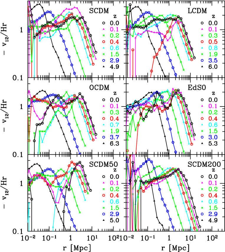
Figure 1: The normalized mean-pairwise peculiar velocity, $-v_{12}/Hr$ as a function of the pair separation $r$ at different redshifts.

Figure 1 shows the scale-dependence of the normalized mean-pairwise peculiar velocity, $-v_{12}(r)/Hr$, at different redshifts ($z\lower 2.15277pt\hbox{$\;\buildrel<\over{\sim}\;$}6$). In linear regimes, the peculiar velocity of pairs $v_{12}(r)$ is negative but smaller than the Hubble velocity $Hr$, and thus the pair-separation still increases in physical length. As clustering proceeds, a given object starts collapsing which corresponds to $-v_{12}(r)/Hr>1$. After experiencing this collapse phase, the system reaches quasi-equilibrium close to $-v_{12}(r)/Hr=1$. As Figure 1 illustrates, the ratio seems to approach $-v_{12}(r)/Hr=1$ (the stable condition) at $r\rightarrow 0$ in all models, but only with significant scatter and variations.

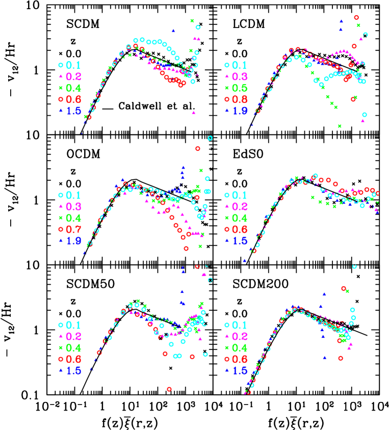
Figure 2: The normalized mean-pairwise peculiar velocity, $-v_{12}/Hr$ as a function of $f(z)\bar{\xi}(r;z)$ at different redshifts. Sold lines indicate the fitting formula proposed by Caldwell et al. (2001).

Figure 2 replots the same data of Figure 1 as a function of $f(z)\bar{\xi}(r,z)$ at different epochs ($z\lower 2.15277pt\hbox{$\;\buildrel<\over{\sim}\;$}2$), following the scaling of Caldwell et al. (2001), where $f(z)$ is the logarithmic derivative of the linear growth rate with respect to the cosmic scale factor. The solid lines in the figure indicate the fitting formula of Caldwell et al. (2001). In the linear and quasi-nonlinear regimes where $f(z)\bar{\xi}(r,z)\lower 2.15277pt\hbox{$\;\buildrel<\over{\sim}\;$}10$, our results are in good agreement with the scaling. In more strongly nonlinear regimes, however, the ratio $-v_{12}(r)/Hr$ varies significantly as a function of $r$ and $z$, and especially shows somewhat irregular oscillatory behavior in time. In those regimes, our results marginally reproduce the fitting formula of Caldwell et al. (2001) only after averaging over time and/or ensembles. Even then the small but systematic deviation from the fitting formula is visible, especially in OCDM model, which might be explained by the difference of the method of estimating $-v_{12}(r)/Hr$; Figure 2 in Jain (1997) shows the similar systematic deviation between the direct estimate and that computed using the pair-conservation equation. In fact, the degree of those variations sensitively depends on the size of the simulation volume itself. Comparison of the SCDM models with $R=50$, 100, and 200 Mpc shows that the variation becomes systematically smaller because of the statistical average over the larger volume. On the other hand, the spatial resolution of the SCDM200 model is not so good as SCDM50, and cannot probe the strongly nonlinear scales corresponding to $f(z)\bar{\xi}(r,z)\lower 2.15277pt\hbox{$\;\buildrel>\over{\sim}\;$}1000$.

For the same reason, Caldwell et al. (2001) remarked that their formula is valid for $f(z)\bar{\xi}(r,z)\lower 2.15277pt\hbox{$\;\buildrel<\over{\sim}\;$}1000$, and that it is not clear whether $-v_{12}(r)/Hr$ converges to unity or possibly oscillates beyond the value. Our result in Figure 2 indicates that the ratio shows an appreciable oscillation even for $f(z)\bar{\xi}(r,z)\lower 2.15277pt\hbox{$\;\buildrel>\over{\sim}\;$}100$. Nevertheless its time-average in all models is not inconsistent with the stable condition asymptotically, i.e., at $f(z)\bar{\xi}(r,z)=(1000\sim 10000)$, and we interpret this to suggest that the stable condition is satisfied after averaging over the cosmological volume.

3.2 Time-variation

In order to understand the origin of the significant variation of $-v_{12}(r)/Hr$, we plot the ratio at fixed physical separations against the cosmic time in units of the present value $t_{0}$ (Fig.3). As the clustering in the corresponding scale proceeds, $-v_{12}(r)/Hr$ monotonically increases in early epochs, but once the separation becomes below the typical collapse scale corresponding to $f(z)\bar{\xi}(r,z)\sim 10$, $-v_{12}(r)/Hr$ exceeds unity and then starts sporadic oscillations.

Jain (1997) also noticed that the direct estimate of the mean-pair wise velocity is quite noisy in his simulations adopting very different gravity solver, integration scheme and the boundary condition from our present ones. We still suspect that the numerical errors due to the two-body relaxation and the integration scheme are not negligible at scales much less than $0.1$Mpc where the Hubble flow amounts to $\sim 10$km/s while the peculiar velocity dispersion exceeds $\sim 500$km/s. Therefore our results below those scales, corresponding to $f(z)\bar{\xi}(r,z)>10^{3}$ at $z=0$, may be interpreted with caution. Nevertheless the significant time-variation is visible even for $f(z)\bar{\xi}(r,z)>10$. Those facts mentioned above suggest that the significant time-variation is not due to any numerical artifact.

We ran several other models with different power spectra, number of particles, and simulation boxsizes, and found that the time-variation persists in all cases, and even becomes stronger for smaller volume runs. This is clearly exhibited for the SCDM50 model in Figure 3. We interpret this behavior as a result of the continuous merging of small-scale objects in the hierarchical clustering universe. Once an over-dense region decouples from the cosmic expansion and becomes self-gravitating, it tends to approach a state of the virial equilibrium, at least temporarily. Such a system, however, is rarely isolated, but rather forms a part an over-dense region on larger scales. Therefore it subsequently experiences disruption and moves to another state of the virial equilibrium corresponding to the higher dynamical temperature in the course of hierarchical merging. Such dynamical behavior should exhibit s significant time-variation if traced at a fixed physical separation. Thus the true mean-pairwise velocity can be estimated only by averaging over a huge cosmological volume; our results imply that the average over $\sim(100$Mpc$)^{3}$ is not still robust and that at least $\lower 2.15277pt\hbox{$\;\buildrel>\over{\sim}\;$}(200$Mpc$)^{3}$ is required to have a reliable estimate for $v_{12}(r)$ even on scales below 1Mpc.

4 Conclusions and discussion

Using a series of high-resolution $N$-body simulations performed in physical coordinates, we compute the mean-pairwise peculiar velocity profile directly from the particle data. In linear and quasi-nonlinear regimes, we confirmed that our simulation data obey the scaling and the fitting formula proposed by Caldwell et al. (2001). In the highly nonlinear regime where the stable condition is conventionally assumed, we found a significant time-variation in the normalized mean-pairwise peculiar velocity $-v_{12}(r)/Hr$, i.e., the stable condition for the physical pair-separation is not stable in time. This behavior can be understood as a natural consequence of the continuous merging processes in the hierarchical clustering universe. This variation can be reduced only by the ensemble average over the cosmological volume $\lower 2.15277pt\hbox{$\;\buildrel>\over{\sim}\;$}(200{\rm Mpc})^{3}$. This is in a sense surprising since the two-point correlation function is a fairly stable statistics and their sample-to-sample variation is not so big (Itoh, Suginohara, & Suto, 1992). On the other hand, our results do not exhibit any clear signal for the systematic departure from the stable condition given the large time-variation. Thus we conclude that while the mean-pairwise peculiar velocity is rather unstable statistics, the stable condition is still valid after the averaging over the entire volume of the universe.

Combined with the fact that the stable condition seems to be satisfied in individual isolated halos (Jing 2001), our results rule out some recent claims that $-v_{12}(r)/Hr$ approaches an asymptotic value smaller than $1/2$ (Kanekar 2000), but may not be inconsistent with the weaker departure predicted by Ma & Fry (2000). Considering the intrinsic nature of the origin for the time-variation, a more definitive answer for the validity of the stable condition for cosmologically averaged pairs requires numerical simulations which have both the higher mass-resolution and the larger simulation volume than our current runs.

Table 1: Simulation parameters

Model	$\Omega_{0}$	$\lambda_{0}$	$h$	$P(k)$	amplitude	$1+z_{i}$	$m$($M_{\odot}$)
SCDM	1.0	0.0	0.5	$\Gamma=0.5$	$\sigma(8h^{-1}{\rm Mpc})=0.6$	25.0	$3.3\times 10^{10}$
LCDM	0.3	0.7	0.7	$\Gamma=0.21$	$\sigma(8h^{-1}{\rm Mpc})=1.0$	33.3	$1.9\times 10^{10}$
OCDM	0.3	0.0	0.7	$\Gamma=0.21$	$\sigma(8h^{-1}{\rm Mpc})=1.0$	33.3	$1.9\times 10^{10}$
EdS0	1.0	0.0	0.5	$n=0$	$\sigma(8h^{-1}{\rm Mpc})=0.6$	100.0	$3.3\times 10^{10}$
SCDM50	1.0	0.0	0.5	$\Gamma=0.5$	$\sigma(8h^{-1}{\rm Mpc})=0.6$	30.0	$4.1\times 10^{9}$
SCDM200	1.0	0.0	0.5	$\Gamma=0.5$	$\sigma(8h^{-1}{\rm Mpc})=0.6$	25.0	$2.6\times 10^{11}$

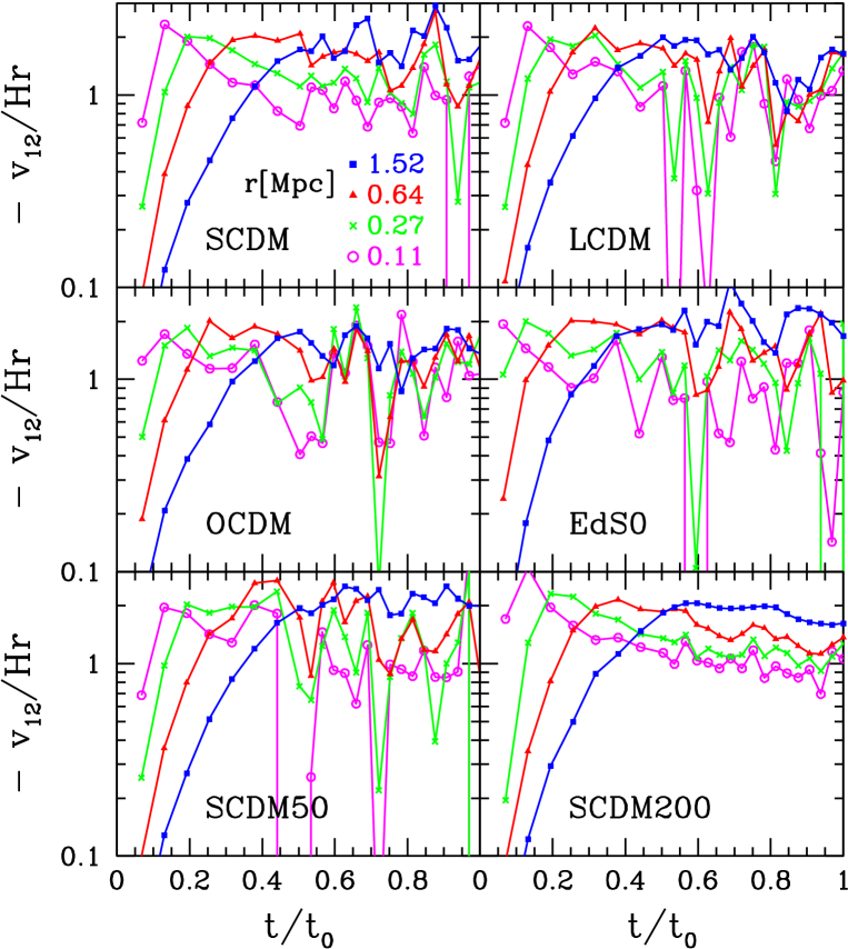
Figure 3: Evolution of $-v_{12}/Hr$ at fixed pair separations $r=0.11$, 0.27, 0.64 and 1.52 Mpc in physical coordinates against the cosmic time.

References

- Barnes (1990) Barnes, J. E. 1990, J. Comp. Phys., 87, 161
- Barnes & Hut (1986) Barnes, J. E., & Hut, P. 1986, Nature, 824, 446
- Caldwell et al. (2001) Caldwell, R.R., Juszkiewicz, R., Steinhardt, P.J., & Bouchet, F.R. 2001, ApJ, 547, L93
- Couchman, Thomas, & Pearce (1995) Couchman, H. M. P., Thomas, P. A., & Pearce, F. R. 1995, ApJ, 452, 797
- Davis & Peebles (1977) Davis, M. & Peebles, P. J. E. 1977, ApJS, 34, 425
- Fukushige & Maino (1997) Fukushige, T. & Makino, J. 1997, ApJ, 477, L9
- Fukushige & Maino (2001) Fukushige, T. & Makino, J. 2001, ApJ, in press (astro-ph/0008104)
- Hamilton et al. (1991) Hamilton, A.J.S., Matthews, A., Kumar, P., & Lu, E. 1991, ApJ, 374, L1
- Itoh, Suginohara, & Suto (1992) Itoh, M., Suginohara, T., & Suto, Y. 1992, PASJ, 44, 481
- Jain, Mo & White (1995) Jain, B., Mo, H. J. & White, S. D. M. 1995, MNRAS, 276, L25
- Jain (1997) Jain, B. 1997, MNRAS, 287, 687
- Jing (2001) Jing, Y.P. 2001, ApJ, 550, L125
- Kanekar (2000) Kanekar, N. 2000, ApJ, 531, 17
- Kawai et al. (2000) Kawai, A., Fukushige, T., Makino, J., & Taiji, M. 2000, PASJ, 52, 659
- Kitayama & Suto (1997) Kitayama, T., & Suto, Y. 1997, ApJ, 490, 557
- Ma & Fry (2001) Ma, C.P. & Fry, J.N. 2001, ApJ, 538, L107
- Makino (1991) Makino, J. 1991, PASJ, 43, 621
- Nityananda & Padmanabhan (1994) Nityananda, R., & Padmanabhan, T. 1994, MNRAS, 271, 976
- Peacock & Dodds (1996) Peacock, J.A. & Dodds, S.J. 1996, MNRAS, 280, L19
- Suginohara, Suto, Bouchet & Hernquist (1991) Suginohara, T., Suto, Y., Bouchet, F. R. & Hernquist, L. 1991, ApJS, 75, 631
- Suginohara, Taruya, & Suto (2001) Suginohara, T., Taruya, A., & Suto, Y. 2001, ApJ, submitted
- Suto (1993) Suto, Y. 1993, Prog.Theor.Phys. 90, 117
- Suto & Jing (1997) Suto, Y. & Jing, Y. P. 1997, ApJS, 110, 167
- Yano & Gouda (2000) Yano, T. & Gouda, N. 2000, 539, 493