Theory of GRB Afterglow

Abstract

The most interesting current open question in the theory of GRB afterglow is the propagation of jetted afterglows during the sideway expansion phase. Recent numerical simulations show hydrodynamic behavior that differs from the one suggested by simple analytic models. Still, somewhat surprisingly, the calculated light curves show a ‘jet break’ at about the expected time. These results suggest that the expected rate of orphan optical afterglows should be smaller than previously estimated.

1 Introduction

Our understanding of GRBs has been revolutionized by the BeppoSAX discovery of GRB afterglow. While GRBs last seconds or minutes the afterglow lasts days, weeks months or even years. This makes afterglow observations much richer. These observations provide us with multi-wavelength and multi-timescales data. At the same time the afterglow, which is a blast wave propagating into the surrounding matter is a much simpler phenomena than the GRB and it is possible to construct a simple theory that can be compared directly with the observations.

In this short review we describe the theory of GRB afterglow. We begin with the simplest idealized model and continue with various levels of complications. The final level is full numerical simulations. We present preliminary results of such simulations and compare them with analytic models. At present there is no simple analytic explanation for the features seen in the numerical results.

2 Spherical Hydrodynamics

The theory of relativistic blast waves has been worked out in a classical paper by Blandford & McKee (BM) already in 1976 BM76 . The BM model is a self-similar spherical solution describing an adiabatic ultra relativistic blast wave in the limit $\Gamma\gg 1$. The basic solution is a blast wave propagating into a constant density medium. However, Blandford and McKee also describe in the same paper a generalization for varying ambient mass density, $\rho=AR^{-k}$, $R$ being the distance from the center. The latter case would be particularly relevant for $k=2$, as expected in the case of wind from a progenitor, prior to the GRB explosion.

The BM solution describes a narrow shell of width $\sim R/\Gamma^{2}$, in which the shocked material is concentrated, where $\Gamma$ is the typical Lorentz factor. The conditions in this shell can be approximated if we assume that the shell is homogeneous. Then the adiabatic energy conservation yields:

$$E={\Omega\over 3-k}AR^{3-k}\Gamma^{2}c^{2}\ ,$$ (1)

where $E$ is the energy of the blast wave and $\Omega$ is the solid angle of the afterglow. For a full sphere $\Omega=4\pi$, but it can be smaller if the expansion is conical with an opening angle $\theta$: $\Omega=2\pi\theta^{2}$ (assuming a double sided jet).

A natural length scale, $l=\left[(3-k)E/\Omega Ac^{2}\right]^{1/(3-k)}$, appears in equation 1. For a spherical blast wave $\Omega$ does not change with time, and when the blast wave reaches $R=l$ it collects ambient rest mass that equals its initial energy, the Lorentz factor $\Gamma$ drops to 1 and the blast wave becomes Newtonian. The BM solution is self-similar and assumes $\Gamma\gg 1$. Obviously, it breaks down when $R\sim l$. We therefore expect that a Relativistic-Newtonian transition should take place around $t_{\rm NR}=l/c\approx 1.2\,{\rm yr}(E_{\rm iso,52}/n_{1})^{1/3}$, where the scaling is for $k=0$, $E_{52}$ is the isotropic equivalent energy, $E_{\rm iso}=4\pi E/\Omega$, in units of $10^{52}{\rm ergs}$ and $n_{1}$ is the external density in ${\rm cm}^{-3}$. After this transition the solution will turn into the Newtonian Sedov-Tailor solution. Clearly this produces an achromatic break in the light curve.

The adiabatic approximation is valid for most of the duration of the fireball. However, during the first hour or so (or even for the first day, for $k=2$), the system could be radiative (provided that $\epsilon_{e}\approx 1$). During a radiative phase the evolution can be approximated as:

$$E={\Omega\over 3-k}AR^{3-k}\Gamma\Gamma_{0}c^{2}\ ,$$ (2)

where $\Gamma_{0}$ is the initial Lorentz factor. Cohen, Piran & Sari CPS98 derived an analytic self-similar solution describing this phase. Cohen & Piran CP99 describe a solution for the case when energy is continuously added to the blast wave by the central engine, even during the afterglow phase. A self-similar solution arises if the additional energy deposition behaves like a power law. This would arise naturally in some models, e.g. in the pulsar like model Usov94 .

3 Spherical Afterglow Models

A good model for the observed emission from spherical blast waves can be obtained by adding synchrotron radiation to these hydrodynamic models. Sari, Piran & Narayan SPN98 used the simple adiabatic scaling (1) together with synchrotron radiation model and the relation between the observer time $t$, and $R$:

$$t=R/C_{1}c\Gamma^{2}\ ,$$ (3)

where $C_{1}$ is a constant that may vary from $2$ to $16$ Sari97 .

Assuming a powerlaw energy distribution of the shocked relativistic electrons: $N(E_{e})\propto E_{e}^{-p}$, and that the electrons and the magnetic field energy densities are $\epsilon_{e}$ and $\epsilon_{B}$ times the total energy density, Sari, Piran & Narayan SPN98 estimate the observed emission as a series of power law segments (PLSs), where

$$F_{\nu}\propto t^{-\alpha}\nu^{-\beta}\ ,$$ (4)

that are separated by break frequencies, across which the exponents of these power laws change: the cooling frequency, $\nu_{c}$, the typical synchrotron frequency $\nu_{m}$ and the self absorption frequency $\nu_{sa}$. The analytic calculations were done for a homogeneous shell and for emission from a single representative point. At a specific frequency one will observe a break in the light curve when one of these break frequencies passes the observed frequency. An intriguing feature of this model is that for a given PLS, say for emission above the cooling frequency, there is a unique relation between $\alpha$, $\beta$ and $p$. The power law index $p$ is expected to be a universal quantity as it depends on the, presumably common, acceleration processes and it is expected to be between 2 and 2.5 SP97 . The consistency of those observed parameters could be a simple check of the theory.

The simple solution, that is based on a homogeneous shell approximation, can modified by using the full BM solution and integrating over the entire volume of shocked fluid GPS99 . Such an integration can be done only numerically. It yields a smoother spectrum and light curve near the break frequencies, but the asymptotic slopes, away from the break frequencies and the transition times, remain the same as in the simpler theory.

Chevalier & Lee CheLi99 estimated the emission from a blast wave propagating into a wind profile $n(R)\propto R^{-2}$. They use equation (1) and calculate the synchrotron emission from a single representative point. This leads to different temporal scalings $\alpha$ of the PLSs, while the spectral indices $\beta$ remain the same, since they are independent of the hydrodynamic solution. This results in different relations between $\alpha$, $\beta$ and $p$, providing in principle a way to distinguish between different neighborhoods of GRBs and between different progenitor models.

Another modification to the ”standard” model arises from a variation of the emission process. Sari & Esin SariEsin01 considered the influence of Inverse Compton on the observed spectrum. They find that in some cases the additional cooling channel might have a significant effect on the observed spectrum and light curves.

4 Jets

The afterglow theory becomes much more complicated if the relativistic ejecta is not spherical. To model jetted afterglows we consider relativistic matter ejected into a cone of opening angle $\theta$. Initially, as long as $\Gamma\gg\theta^{-1}$ Pi94 the motion would be almost conical. There isn’t enough time, in the blast wave’s rest frame, for the matter to be affected by the non spherical geometry, and the blast wave will behave as if it was a part of a sphere. When $\Gamma=C_{2}\theta^{-1}$, namely at:

$$t_{\rm jet}={1\over C_{1}}\left(l\over c\right)\left({\theta\over C_{2}}\right)^{2(4-k)\over(3-k)}={1\,{\rm day}\over C_{1}C_{2}^{8/3}}\left({E_{\rm iso,52}\over n_{1}}\right)^{1/3}\left({\theta\over 0.1}\right)^{8/3}\ ,$$ (5)

rapid sideway propagation begins. The last equality holds, of course for $k=0$.

The sideways expansion continues with $\theta\sim\Gamma^{-1}$. Plugging this relations in equation (1) we find that $R\approx{\rm const}.$ This is obviously impossible. A more detailed analysis Rhoads99 ; Pi00 ; KP00 reveals that according to the simple one dimensional analytic models $\Gamma$ decreases exponentially with $R$ on a very short length scale.

The sideways expansion causes a change in the hydrodynamic behavior and hence a break in the light curve. Additionally, when $\Gamma\sim\theta^{-1}$ relativistic beaming of light will become less effective. This would cause an extra spreading of the emission (that was previously focused into a narrow angle $\theta$ and is now focused into a larger cone of opening angle $\Gamma^{-1}$). If the sideways expansion is at the speed of light than both transitions would take place at the same time SPH99 . If the sideways expansion is at the sound speed then the beaming transition would take place first and only later the hydrodynamic transition would occur PM99 . This would cause a slower and wider transition with two distinct breaks, the first and steeper break when the edge of the jet becomes visible and later a shallower break when sideways expansion becomes important.

The analytic or semi-analytic calculations of synchrotron radiation from jetted afterglows Rhoads99 ; SPH99 ; PM99 ; MSB00 ; KP00 have led to different estimates of the jet break time $t_{\rm jet}$ and of the duration of the transition. Rhoads Rhoads99 calculated the light curves assuming emission from one representative point, and obtained a smooth ’jet break’, extending $\sim 3-4$ decades in time, after which $F_{\nu>\nu_{m}}\propto t^{-p}$. Sari Piran & Halpern SPH99 assume that the sideway expansion is at the speed of light, and not at the speed of sound ($c/\sqrt{3}$) as others assume, and find a smaller value for $t_{\rm jet}$. Panaitescu and Mészáros PM99 included the effects of geometrical curvature and finite width of the emitting shell, along with electron cooling, and obtained a relatively sharp break, extending $\sim 1-2$ decades in time, in the optical light curve. Moderski, Sikora and Bulik MSB00 used a slightly different dynamical model, and a different formalism for the evolution of the electron distribution, and obtained that the change in the temporal index $\alpha$ ($F_{\nu}\propto t^{-\alpha}$) across the break is smaller than in analytic estimates ($\alpha=2$ after the break for $\nu>\nu_{m}$, $p=2.4$), while the break extends over two decades in time. Kumar and Panaitescu KP00 find that for a homogeneous (or stellar wind) environment there is a steepening of $\Delta\alpha\sim 0.7$ ($0.4$) when the edge of the jet becomes visible, while the steepening due to sideways expansion extends over 2 (4) decades in time. They conclude that a jet running into a stellar wind will not leave a prominent detectable signature in the light curve.

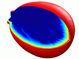
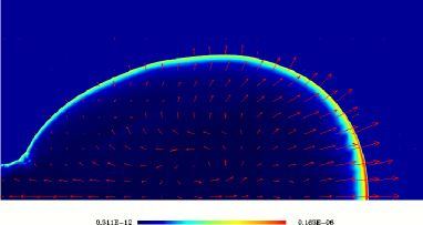
Figure 1: A relativistic jet at the last time step of the simulation Granot01 . (left) A 3D view of the jet. The outer surface represents the shock front while the two inner faces show the proper number density (lower face) and proper emissivity (upper face) in a logarithmic color scale. (right) A 2D ’slice’ along the jet axis, showing the velocity field on top of a linear color-map of the lab frame density.

The different analytic or semi-analytic models have different predictions for the sharpness of the ’jet break’, the change in the temporal decay index $\alpha$ across the break and its asymptotic value after the break, or even the very existence a ’jet break’ HDL00 . All these models rely on some common basic assumptions, which have a significant effect on the dynamics of the jet: (i) the shocked matter is homogeneous (ii) the shock front is spherical (within a finite opening angle) even at $t>t_{\rm jet}$ (iii) the velocity vector is almost radial even after the jet break.

However, recent 2D hydrodynamic simulations Granot01 show that these assumptions are not a good approximation of a realistic jet. Figure 1 shows the jet at the last time step of the simulation. The matter at the sides of the jet is propagating sideways (rather than in the radial direction) and is slower and much less luminous compared to the front of the jet. The shock front is egg-shaped, and quite far from being spherical. Figure 2 shows the radius $R$, Lorentz factor $\Gamma$, and opening angle $\theta$ of the jet, as a function of the lab frame time. The rate of increase of $\theta$ with $R\approx ct_{\rm lab}$, is much lower than the exponential behavior predicted by simple models Rhoads99 . The value of $\theta$ averaged over the emissivity is practically constant, and most of the radiation is emitted within the initial opening angle of the jet. The radius $R$ weighed over the emissivity is very close to the maximal value of $R$ within the jet, indicating that most of the emission originates at the front of the jet, where the radius is largest, while $R$ averaged over the density is significantly lower, indicating that a large fraction of the shocked matter resides at the sides of the jet, where the radius is smaller. The Lorentz factor $\Gamma$ averaged over the emissivity is close to its maximal value, (again since most of the emission occurs near the jet axis where $\Gamma$ is the largest) while $\Gamma$ averaged over the density is significantly lower, since the matter at the sides of the jet has a much lower $\Gamma$ than at the front of the jet. The large differences between the assumptions of simple dynamical models of a jet and the results of 2D simulations, suggest that great care should be taken when using these models for predicting the light curves of jetted afterglows. Since the light curves depend strongly on the hydrodynamics of the jet, it is very important to use a realistic hydrodynamic model when calculating the light curves.

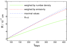
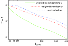
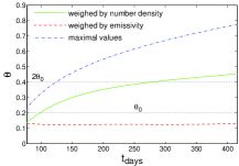
Figure 2: The radius $R$ (left frame), Lorentz factor $\Gamma-1$ (middle frame) and opening angle $\theta$ of the jet (right frame), as a function of the lab frame time in days Granot01 .

Granot et al. Granot01 used 2D numerical simulations of a jet running into a constant density medium to calculate the resulting light curves, taking into account the emission from the volume of the shocked fluid with the appropriate time delay in the arrival of photons to different observers. They obtained an achromatic jet break for $\nu>\nu_{m}(t_{\rm jet})$ (which typically includes the optical and near IR), while at lower frequencies (which typically include the radio) there is a more moderate and gradual increase in the temporal index $\alpha$ at $t_{\rm jet}$, and a much more prominent steepening in the light curve at a latter time when $\nu_{m}$ sweeps past the observed frequency. The jet break appears sharper and occurs at a slightly earlier time for an observer along the jet axis, compared to an observer off the jet axis (but within the initial opening angle of the jet). The value of $\alpha$ after the jet break, for $\nu>\nu_{m}$, is found to be slightly larger than $p$ ($\alpha=2.85$ for $p=2.5$).

Somewhat surprisingly we find that in spite of the different hydrodynamic behavior the numerical simulations show a jet break at roughly the same time as the analytic estimates. This encourages us to trust the current estimates of the jet opening angles. However, we should search for an intuitive explanation for the nature of the hydrodynamic behavior and for a simple analytic model that would predict it.

References

- (1) R.D. Blandford, C.F. McKee: Phys. of Fluids, 19, 1130 (1976).
- (2) E. Cohen, T. Piran, R. Sari: Ap. J., 509, 717 (1998).
- (3) E. Cohen, T. Piran: Ap. J., 518, 346 (1999).
- (4) V.V. Usov: MNRAS, 267,1035 (1994)
- (5) R. Sari, T. Piran, R. Narayan: Ap. J. Lett., 497, L17 (1998).
- (6) R. Sari: Ap. J. Lett., 489, L37 (1997).
- (7) R. Sari, T. Piran: MNRAS, 287, 110 (1997).
- (8) J. Granot, T. Piran, R. Sari: Ap. J., 513, 679 (1999).
- (9) R.A. Chevalier, Z.-Y. Li: Ap. J. Lett., 520, L29 (1999).
- (10) R. Sari, A.A. Esin: Ap. J., 548, 787 (2001).
- (11) T. Piran: in AIP Conference Proceedings 307, Gamma-Ray Bursts, Second Workshop, Huntsville, Alabama, 1993, Fishman, G.J., Brainerd, J.J., & Hurley, K., Eds., (New York: AIP), p. 495. (1994)
- (12) J.E. Rhoads: Ap. J., 525, 737 (1999)
- (13) T. Piran: Phys. Rep., 333, 529 (2000)
- (14) P. Kumar & A. Panaitescu: Ap. J., 541, L9 (2000)
- (15) R. Sari, T. Piran, T. Halpern: Ap. J., 519, L17 (1999).
- (16) A. Panaitescu & P. Mészáros: Ap. J., 526, 707 (1999)
- (17) R. Moderski, M. Sikora, T Bulik: Ap. J., 529, 151 (2000)
- (18) Y. Huang, Z. Dai & T. Lu: A&A 355, L43 (2000)
- (19) J. Granot, et al.: These proceedings (astro-ph/0103038) (2001)