Quantum Gravity and Astrophysics: The Microwave Background and Other Thermal Sources

Abstract

The problem of formulating a fully consistent quantum theory of gravity has not yet been solved. Even before we are able to work out the details of a complete theory, however, we do know some important qualitative features to be expected in any quantum theory. Fluctuations of the metric, for example, are expected and are associated with fluctuations of the lightcone. Lightcone fluctuations affect the arrival time of signals from distant sources in potentially measurable ways, broadening the spectra. In the work described here, we start with a thermal spectrum and derive the form of spectral changes expected in a wide class of quantum theories of gravity. The results can be applied to any thermal spectrum. We focus on their application to the cosmic microwave background (CMB) because the CMB offers two advantages: (1) deviations from a thermal spectrum are well constrained, and (2) the radiation emanates from the most distant source of light, the surface of last scattering. We use the existing CMB data to derive an upper bound on the value of $\Delta\,t,$ the mean spread in arrival times due to metric fluctuations: ${\Delta t}<2.1\times 10^{-14}$ s at the $95\%$ confidence limit. This limit applies to a wide range of quantum theories of gravity, and thus serves to falsify theories predicting a larger spread in arrival times. We find this limit rules out at least one quantum gravity theory, the 5-dimensional quantum theory in which the “extra” dimension is flat. Meaningful tests of many other models may also be possible, depending on the results of calculations to predict values of $\Delta\,t,$ and also a second time scale $\tau_{c},$ the correlation time, which is the characteristic time scale of the metric fluctuations. We show that stronger limits on the value of $\Delta\,t,$ and hence on the effects of lightcone fluctuations, are likely to be derived through observations of higher-temperature sources, especially in the X-ray and gamma-ray regimes.

1 Introduction

Because the theory of gravity describes the spacetime itself, quantization of gravity is conceptually more difficult than quantization of the other fundamental interactions. If, however, the basic quantum principles we are already familiar with apply as well to a quantum theory of gravity, we can make some predictions about expected quantum effects, even in the absence of a fundamental underlying theory. Indeed, if some such predictions can be tested, we may be able to derive useful constraints on the properties of the true underlying theory in which gravity is quantized. The basic question we pose here is whether data received from astrophysical systems emitting thermal radiation can provide tests of quantum gravity.

One generic prediction is that the quantization of gravity should be associated with fluctuations of the spacetime metric. Let the classical spacetime metric be represented by $\bar{g}_{\mu\nu}=\eta_{\mu\nu}$, and let the fluctuations be described by $h_{\mu\nu}.$ The full quantum metric, $g_{\mu\nu}$, is therefore the sum: $g_{\mu\nu}=\eta_{\mu\nu}+h_{\mu\nu}$. The fluctuations described by $h_{\mu\nu}$ can be viewed as leading to fluctuations of the lightcone. Lightcone fluctuations cause the arrival times of light signals to differ from what they would have been in the classical theory. The arrival times are not systematically earlier or later than those predicted classically, but are instead spread about the classical prediction in both directions. See Figure 1. The functional form of the mean spread, $\Delta t$, is determined by the functional form of $h_{\mu\nu}$. Because increasing path length provides more opportunities for lightcone fluctuations to act, $\Delta t$ typically grows with increasing distance between the emitter and detector, but the rate of growth can also depend on the geometry and topology of the spacetime.

Figure 1: Imagine several photons emitted from the same spacetime point. The effects of lightcone fluctuations on the paths of these photons are illustrated by plotting the time $t$ taken for light to propagate along a path coordinatized by $x$; the units are arbitrary. The dotted line shows the classical lightcone; eighteen paths subject to lightcone fluctuations are depicted by solid lines. Fluctuations which could either increase or decrease the time of flight were randomly introduced along each path. Note that the mean fluctuation, $\Delta t,$ tends to grow as the path length increases.

A spread in arrival times introduces spectral changes. If, for example, the classical situation is that a perfect wave of one frequency is emitted by some source, lightcone fluctuations will introduce a spread in the arrival times of each peak. This spread is measured as a spread in the frequencies received from the source by a detector. Spectral changes between the emitted and received spectrum of light can be expressed in terms of $\Delta t$.

The purpose of this paper is to compute the form of the changes induced in a thermal spectrum and to consider the astrophysical circumstances under which these changes might be detectable. We focus on the application to the cosmic microwave background. Our motivation for this application is twofold. First, deviations of the CMB from a pure thermal spectrum are well constrained; second, the effect of any given metric fluctuation increases with distance, and the surface of last scattering is the most distant emitter of light. In §2 we start with a given $\Delta t$ and compute the form of the expected spectral deviations. In §3 we apply our results to the microwave background. In §4 we demonstrate how $\Delta t$ can be related to metric fluctuations and thus, how either measuring or placing limits on the size of $\Delta t$ can help to probe quantum fluctuations of the metric. In §5 we study the prospects that astrophysical measurements, including but not limited to measurements of the CMB, will allow us to place useful constraints in the foreseeable future.

It is interesting to consider whether angular dependence due to metric fluctuations, provides another effect which can be used to test quantum gravity. This question is not central to the work we describe on the cocmic microwave background (CMBR), since we are interested in the in the determination of its temperature, and not in the variation of temperature across the sky. Nevertheless, angular effects could be useful in other applications. We therefore consider them in the appendix. We show that, in the quantum gravity theory we have considered, angular deviations are a higher order effect than lightcone fluctuations and can therefore be neglected. In other cases, however, an angular spread due to lightcone fluctuations could turn out to be important; we therefore discuss the implications in §5.1.

2 Deviations from a Thermal Spectrum Due to Light Cone Fluctuations

A classical pulse of light will propagate through a distance $r$ in time $r/c=r,$ where, in this last equality, we have introduced units with $c=1.$ Lightcone fluctuations cause propagation times to be either longer or shorter than $r$ by a mean deviation $\Delta t.$

$$\Delta t={{\sqrt{\langle\sigma_{1}^{2}\rangle}}\over{r}},$$ (1)

where ${\langle\sigma_{1}^{2}\rangle}$ is the mean square deviation in the geodesic interval function.

The functional form of $\Delta\,t$ and the range of its expected values emerge from specific quantum theories. In general, $\langle\sigma_{1}^{2}\rangle$ is a function of the flight time $r$. If the fluctuations were a random walk type of process, one could think of them as occuring in a sequence of steps, each of which is uncorrelated with the previous step. In this case, one would have $\langle\sigma_{1}^{2}\rangle\propto r^{2}$ and $\Delta t\propto\sqrt{r}$. However, quantum metric fluctuations are not necessarily of this type, and detailed models can lead to other functional dependencies of $\Delta t$ upon $r$. One class of models which can lead to large lightcone fluctuations are Kaluza-Klein type theories with compact extra dimensions. Confining a quantum field into a region with a small compact spatial dimension leads to enhanced quantum fluctuations, as a consequence of the uncertainty principle. This issue, and the details of how $\langle\sigma_{1}^{2}\rangle$ is calculated will be discussed in more detail in §4. Another issue also discussed there is that of the correlation time, $\tau_{c}$. The expected relative time delay or advance of a pair of pulses is only given by $\Delta t$ when the pulses are separated in time by an amount greater than $\tau_{c}$, which one can regard as the characteristic time scale for the metric fluctuations.

Here we assume Gaussian fluctuations and that $\Delta t$ is frequency independent. This is a natural choice, and corresponds to the achromaticity of gravitational effects in classical general relativity. The choices of frequency-independence and Gaussianity are more specifically motivated by work (Ford 1995) showing that linear quantum metric fluctuations due to a bath of gravitons modifies the retarded Green’s function from a delta function on the forward lightcone into a Gaussian function. In addition, the same behavior was found by Yu and Ford (1999) in models in which the metric fluctuations arise from compact extra dimensions. In both of these cases, the resulting $\Delta t$ is found to be frequency-independent. Thus, although the assumptions of frequency-dependence and Gaussianity are not universally applicable, they do apply to important classes of theories and are likely to provide useful insights into the effects of lightcone fluctuations in other classes of quantum gravity theories. We further note that, although some quantum gravity theories do predict frequency dependent effects (Amelino-Camelia et al. 1998), astronomical data is already beginning to place limits on such frequency-dependence. For example, observations of the Crab pulsar rule out differential time delays greater than $0.35$ msec for energies above $2$ GeV as compared with $70-100$ MeV (Kaaret 1999). Study of a TeV $\gamma$-ray flare associated with the active galaxy Markarian 421 indicates that there is no significant time delay between the emission at $1$ TeV and the emission at $2$ TeV (Biller et al. 1999). Multiwavelength observations of $\gamma$-ray bursts can place even stronger limits on the frequency-dependence of lightcone fluctuations if simultaneous observation of the arrival times from radio to $\gamma$-ray energies can be made, and if the distance to the burst source can be determined (Schaefer 1999). We therefore proceed with calculations incorporating the choices of frequency-independence and Gaussianity, which simplify the calculations and also allow us to determine what functional forms for the frequency dependence can be most readily tested.

A spread in flight times for pulses necessarily implies a spread in frequency. Consider, for example, a source which emits a monchromatic wave. The individual wave crests may be regarded as being pulses whose times of arrival at a detector vary by about $\Delta t$. This introduces a spread in frequency, $\Delta\nu$. This means that we can look for signatures of lightcone fluctuations in the frequency domain rather than the time domain, which is likely to lead to more stingent constraints. Even a staionary source such a blackbody emitter, which does not have any intrinsic time dependence, can have its frequency spectrum distorted by lightcone fluctuations.

When there are Gaussian lightcone fluctuations, a monochromatic wave of frequency $\nu_{0}=1/T_{0},$ with $T_{0}$ the period, becomes a Gaussian with width

$$|\Delta\,\nu|={{\Delta\,t}\over{T_{0}^{2}}}=\nu_{0}^{2}\,\Delta\,t$$ (2)

That is,

$$\delta(\nu_{0})\longrightarrow\exp\Bigg{[}{-\Big{(}{{\nu-\nu_{0}}\over{\Delta\,\nu}}\Big{)}^{2}}\Bigg{]}{{1}\over{\sqrt{\pi}\Delta\,\nu}}$$ (3)

Thus, a spectrum described by a function $F_{0}(\nu^{\prime})$, is distorted and will now be described by $F(\nu).$ If the original spectrum was thermal, then

$$F_{0}(\nu^{\prime})={{a\,\nu^{\prime 3}}\over{e^{b\,\nu^{\prime}}-1}}$$ (4)

and

$$F(\nu)={{a}\over{\sqrt{\pi}\,\Delta\,t}}\int_{0}^{\infty}d\nu^{\prime}{{\nu^{\prime}}\over{e^{b\,\nu^{\prime}}-1}}\,\exp\Bigg{[}{-\Big{(}{{(\nu^{\prime}-\nu)}\over{\nu^{\prime 2}\Delta\,t}}\Big{)}^{2}}\Bigg{]}.$$ (5)

It is convenient to evaluate this integral by introducing the variable $z,$ defined so that

$$z\,\Delta t=\nu^{\prime}-\nu.$$ (6)

$F(\nu)$ can now be expressed as

$$F(\nu)={{a}\over{\sqrt{\pi}}}\int_{-{{\nu}\over{\Delta\,t}}}^{\infty}dz\,e^{-{{z^{2}}\over{\nu^{4}}}}{{\nu}\over{e^{b\,\nu}-1}}.$$ (7)

Expanding to second order in $\Delta\,t,$ we find that

$$F(\nu)=F_{0}(\nu)\,\Bigg{[}1+f_{2}(\nu)\Bigg{]},$$ (8)

where $f_{2}(\nu)$ may be written as follows:

$$f_{2}(\nu)=f_{2}(x[\nu])=\Bigg{(}{{\Delta\,t}\over{b}}\Bigg{)}^{2}\Bigg{\{}{{x^{2}}\over{4\,(e^{x}-1)^{2}}}\Bigg{[}e^{2\,x}\Big{(}x\,(x-14)+42\Big{)}+e^{x}\Big{(}x\,(x+14)-84\Big{)}+42\Bigg{]}\Bigg{\}},$$ (9)

with

$$x=x(\nu)=b\,\nu\,.$$ (10)

The physical meaning of $f_{2}(x)$ is that it is the fractional deviation from a thermal spectrum caused by lightcone fluctuations. It is useful to concentrate on its functional form, independent of the value of $\Delta\,t$ and of the temperature of the emitter. We therefore consider $\hat{f_{2}}(x).$

$$\hat{f_{2}}(x)=f_{2}(x)\ \Big{(}{{b}\over{\Delta\,t}}\Big{)}^{2}\,.$$ (11)

Figure 2 displays the functional form of $\hat{f_{2}}(x)$ for $x<10.$ As $x$ increases, $\hat{f_{2}}$ continues to increase as $x^{4}/4.$ Thus, reliable measurements of a thermal spectrum that extend to high frequencies with small uncertainties have a good chance of detecting any deviations that may exist due to lightcone fluctuations. Since, however, the spectrum is actually falling to zero as $\nu$ increases, high precision measurements may be more difficult. It is therefore instructive to consider $\hat{F_{2}}=F_{0}\,\hat{f_{2}},$ which is plotted in Figure 3. The term that must be added to the original spectrum in order to obtain the perturbed spectrum is simply $\hat{F_{2}}\times({{\Delta\,t}\over{b}})^{2}.$

The effects of lightcone fluctuations on the spectrum can be seen directly in Figures 4 and 5. In Figure 4, $\Delta t/b$ was chosen to be $0.1.$ Note that, as the functional form of $\hat{f_{2}}$ dictates, the flux is enhanced near and below the peak of the thermal spectrum, with a dip at intermediate frequencies, and then a second significant enhancement extending out to higher frequencies. Had the value of $\Delta t/b$ been slightly larger, the flux near $x\sim 8$ would have dipped below $0,$ indicating that the second order approximation we made to derive a simple analytic form is no longer valid. In Figure 5, $\Delta t/b$ was chosen to be $0.01.$ With this choice, the effects at low and intermediate frequency are just visible by eye on a plot linear in the flux, while the effects at higher frequencies can be clearly seen in a logarithmic plot. As $\Delta t/b$ decreases further, sensitive measurements are needed to discover definitive evidence of lightcone fluctuations. In Figure 6, the logarithm of the fractional deviation from a thermal spectrum (expressed in parts per million) is plotted as a function of $x.$ Each curve corresponds to a different value of $\Delta\,t/b$. This plot illustrates the role high-precision measurements of a thermal spectrum can play in measuring or placing limits on the value of $\Delta t.$

Figure 2: $\hat{f_{2}}$ is plotted as a function of $x$. The mean fractional deviation from a pure thermal spectrum is given by $\hat{f_{2}}\times({{\Delta\,t}\over{b}})^{2}$.

Figure 3: $\hat{F_{2}}\times({{\Delta\,t}\over{b}})^{2}$ is the term that must be added to a pure thermal spectrum when there are lightcone fluctuations.

Figure 4: In both the upper and lower panels a pure thermal spectrum (solid curve) is plotted and compared with the perturbed spectrum (dotted curve); the case considered is $(\Delta\,t/b)=0.1$. Note that this value of $(\Delta\,t/b)$ is very close to the maximum value consistent with the approximation we have made in Equation 8; when the value is larger, the flux becomes negative, hence unphysical, for a range of frequencies near $x=8$.

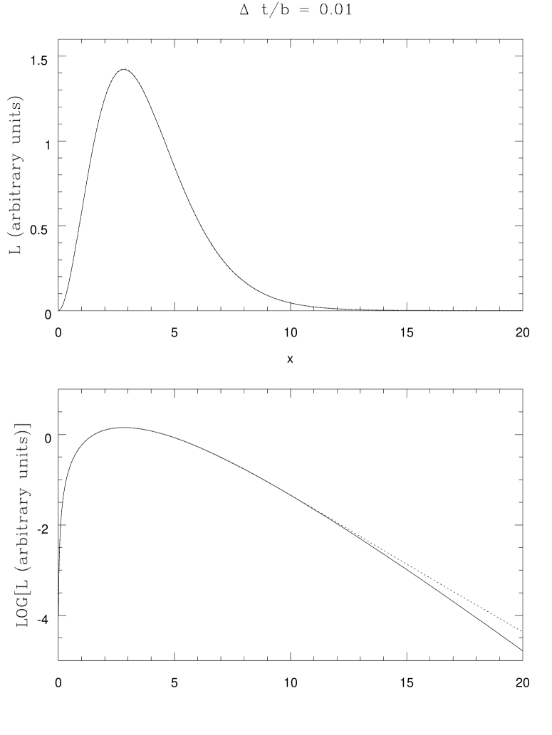
Figure 5: In both the upper and lower panels a pure thermal spectrum (solid curve) is plotted and compared with the perturbed spectrum (dotted curve).

Figure 6: Plotted is log${}_{10}[f_{2}(x)\times 10^{6}]$ vs $x$. Because $f_{2}(x)$ (and not $\hat{f}_{2}(x)$) is plotted, each curve is characterized by a value of $(\Delta\,t/b)$; these values are used to label the curves. As $(\Delta\,t/b)$ decreases, perturbations due to lightcone fluctuations become more difficult to discern by eye. This plot illustrates that precision measurements of the spectral shape can nevertheless be effective in constraining even small values of $(\Delta\,t/b)$. This is particularly so (1) for values of $x$ around extrema in $\hat{f}_{2}(x),$ and (2) at high frequencies, if the thermal spectrum at high frequencies is not contaminated by contributions due to other physical effects.

3 Application to the Microwave Background

The spectrum of the microwave background has been measured by the FIRAS (Far InfraRed Absolute Spectraphotometer) aboard the COBE (Cosmic Background Explorer) over the range of wavelengths (480-4400 $\mu$m [$\nu=2-21$ cm^-1]). These measurements have constrained departures from a pure thermal spectrum at a level of a few parts in $10^{-5}$ near the peak of the spectrum (Fixsen et al. 1996) and the absolute temperature to 2.725$\pm$.002 (95% CL) (Mather et al. 1999). These measurements can be used to constrain the lightcone fluctuations.

$$\Bigg{|}{{\Delta F(x)}\over{F(x)}}\Bigg{|}=\Bigg{|}\hat{f}_{2}(x)\Bigg{|}\times\Bigg{(}{{\Delta\,t}\over{b}}\Bigg{)}^{2}<\Big{|}d(x)\Big{|},$$ (12)

where values of d(x) are on the order of $10^{-5}$ near the peak of the spectrum.

We have used two methods to derive limits on ${{\Delta\,t}\over{b}}$ from the microwave data. First, we proceeded in exact analogy to the work carried out by Fixsen et al. 1996; in that paper limits on Comptonization and on a chemical potential were derived, based on fits to the COBE-measured spectrum. In §3.1, limits on the microwave background are put on the same footing, yielding the $95\%$ confidence limit ${{\Delta\,t}\over{b}}<0.0012$. In §3.2 we take another approach, using a point-by-point analysis. This approach allows us to identify the points that provide the strongest constraints, and show that they produce a result consistent with the result derived by considering the full spectrum. Such a point-wise analysis could be used for other thermal spectra. If, for example, measurements at only a limited number of points are possible, our approach illustrates which are the most useful points to sample. Alternatively, the point-wise approach could strengthen the results based on the microwave data if one or two high-precision spectral measurements of the microwave background can be made at higher frequencies.

3.1 Constraints Based on Spectral Fits

To derive limits for $(\Delta t/b)^{2}$ we linearize the distortion in $(\Delta t/b)^{2}$ to approximate $\Delta F$ as follows. [See Eqs. (8) and (11).]

$$\Delta F(x)=F_{0}(x)\,\hat{f_{2}}(x)\ \Big{(}{{\Delta t}\over{b}}\Big{)}^{2},$$ (13)

where $x=0.5278\,\nu.$ Note that $x,$ which is dimensionless in units with $c=1$, is defined in Equation (10); here we consider the specific case of the microwave background, with $T=2.725K.$

Fixsen et al. (1996) provide a table with residuals ($r$), the $1\,\sigma$ uncertainties ($c$), a galactic template ($G$), and correlations ($Q$). Together with the derivative of the Planck function, $dF_{0}/dT$, we have all of the components required to fit the quantum gravity fluctuations, paralleling the fits appropriate to the other distortions (Fixsen et al. 1996, Eq. 3).

The $dF_{0}/dT$ and galactic spectra are included here (as there) to allow for uncertainty in the temperature (which was determined from the data) and the amount of residual galactic contamination. The full covariance matrix was used (it can be derived from $\sigma$ and $(\Delta t/b)^{2}$). The result of this fit is $(\Delta t/b)^{2}=-1.8\times 10^{-7}\pm 7.1\times 10^{-7}$. Physical measurements of $a$ should yield a non-negative result; since, however, the negative result we have found is only at the level of $-.25\sigma,$ it is likely to represent only statistical errors in the estimation of $a$.

We can then use the derived uncertainty of $a$ to place an upper limit on $a$ and hence on $\Delta t$. For a 95% confidence limit

$$(\Delta t/b)^{2}<2\,(7.1\times 10^{-7}),$$ (14)

$$\Delta t/b<.0012.$$ (15)

Figure 7 illustrates this point. Shown are the measured residuals from the analysis of the FIRAS data; a thermal spectrum with $T=2.725$ K has been subtracted, as has the dipole contribution and the contribution likely to be due to our own Galaxy. The long-dashed curve corresponds to the largest value of the chemical potential (due to energy input before $z=10^{5}$) consistent with the data, and the short-dashed curve corresponds to the maximum effects of Comptonization (occurring after $z=10^{5}$) consistent with the data. as shown in Figure 7. Since $b=1.76\times 10^{-11}$ for $T=2.725~{}$K, this translates to $\Delta t<2.1\times 10^{-14}$ s.

Figure 7: Deviations from a thermal spectrum. The unit along the vertical axis is MJy/sr; the unit along the horizontal axis is the same dimensionless variable $x$ we have been using throughout this paper. We have translated from the frequency units of cm^-1 used by Fixsen et al. (1996): $x=\nu_{Fixsen}\ (h\,c)/(k\,T)$. The jagged line, with data points indicated by the filled circles, shows the measured residuals from the analysis of the FIRAS data; a thermal spectrum with $T=2.725$ K has been subtracted, as has the dipole contribution and the contribution likely to be due to our own Galaxy. The solid curve shows the contribution of lightcone fluctuations for $\Delta\,t/b=0.0012.$ The long-dashed curve corresponds to the largest value of the chemical potential (due to energy input before $z=10^{5}$) consistent with the data, and the short-dashed curve corresponds to the maximum effects of Comptonization (occurring after $z=10^{5}$) consistent with the data.

3.2 Constraints Based on Individual Points

Each measurement at a given frequency (characterized by $x=0.5278\,\nu$), provides a constraint on $\Delta\,t/b.$

$$\log\Bigg{[}{{\Delta\,t}\over{b}}\Bigg{]}<-{{1}\over{2}}\Bigg{\{}\log\Bigg{[}\Big{|}d(x)\Big{|}\Bigg{]}+\log\Bigg{[}\Big{|}\hat{f}_{2}(x)\Big{|}\Bigg{]}\Bigg{\}}.$$ (16)

Thus, to derive the tightest limits (i.e., lowest upper bound) on $\Delta\,t,$ we want to find the minimum value of right-hand side of the above equation consistent with the data.

To do this, we considered each frequency, $\nu,$ at which the microwave background was measured. Let $F(x)$ represent the best-fit thermal spectrum. We estimate $d(x)$ in two ways: $d_{1}(x)=|{r(x)}|/F(x),$ $d_{2}(x)=c(x)/F(x)$, where $r(x)$ represents the residuals and $c(x)$ represents the $1\,\sigma$ uncertainties, respectively. Note that $d_{1}(x)$ and $d_{2}(x)$ are both positive, so we omit the absolute value signs wherever $d(x)$ appears below. For each frequency at which a spectral measurement was made, we define ${{\Delta\,t}\over{b}}(x)_{ul}$ to be that value of ${{\Delta\,t}\over{b}}$ that turns (16) into an equality.

$$\log\Bigg{[}{{\Delta\,t}\over{b}}(x)\Bigg{]}_{ul}=-{{1}\over{2}}\Bigg{\{}\log\Bigg{[}d(x)\Bigg{]}+\log\Bigg{[}\Bigg{|}\hat{f}_{2}(x)\Bigg{|}\Bigg{]}\Bigg{\}}.$$ (17)

In this way, each measurement provides [for each way of measuring $d(x)$] an upper bound on ${{\Delta\,t}\over{b}}.$ The lowest value of the upper bounds so obtained is then the tightest limit that can be derived from this type of point-by-point analysis of the FIRAS data set. Figure 8 illustrates the results. The points shown as open circles are $\{d_{2}(x),{{\Delta\,t}\over{b}}(x)_{ul}\};$ the minimum value of ${{\Delta\,t}\over{b}}(x)$ achieved by any of these points is $0.0015.$ The points shown as crosses are $\{d_{1}(x),{{\Delta\,t}\over{b}}(x)_{ul}\};$ the minimum value of ${{\Delta\,t}\over{b}}(x)_{ul}$ achieved by any of these points is $0.0006.$

The more sophisticated global analysis of the spectrum carried out in §3.1 produces an upper limit that lies between the values obtained by using $d_{1}$ and $d_{2}.$ This can also be illustrated graphically. If, for example, we plotted the curves corresponding to $\Delta\,t/b=0.0006$ and a succession of values up to and including $\Delta\,t/b=0.015$ on this graph, it would be clear that the smaller value is too low and that the upper limit is too high. In fact, such an analysis leads to the result:

$${{\Delta t}\over{b}}<0.001^{+0.0003}_{-.0003}.$$ (18)

Since $b$ (in Equation 10) has the value $1.76\times 10^{-11}$ s for $T=2.725$ K, this translates to

$${\Delta t}<1.8^{+0.5}_{-0.5}\times 10^{-14}\ s.$$ (19)

This is consistent with the results of the more sophisticated analysis of §3.1, demonstrating that reliable results can be derived with an analysis that focuses primarily measurements at a few well-chosen frequencies. By “well-chosen frequencies”, we mean frequencies at which the effects of lightcone fluctuations are maximized, as shown in Figures 2 and 6.

Figure 8: The log of the fractional deviation from a pure thermal spectrum is plotted along the horizontal axis. Along the vertical axis is plotted ${{\Delta t}\over{b}}(x)_{ul}$ (i.e., the upper limit allowed for each value of $x$, as defined in Eq. (17)). Each point shown corresponds to the FIRAS measurement of the microwave background at a particular frequency, $x.$ The points $\{d_{1}(x),{{\Delta\,t}\over{b}}(x)_{ul}\}$, shown as crosses, are determined by the residuals; the minimum value of ${{\Delta\,t}\over{b}}(x)_{ul}$ achieved by any of these points is $0.0006.$ The points $\{d_{2}(x),{{\Delta\,t}\over{b}}(x)_{ul}\}$, shown as open circles, are determined by the standard deviations; the minimum value of ${{\Delta\,t}\over{b}}(x)$ achieved by any of these points is $0.0015.$ The two cusps with the highest values of ${{\Delta\,t}\over{b}}(x)_{ul}$ correspond to values of $x$ for which $\hat{f}_{2}$ is near zero. The continuous lines each plot Eq. (17) for a given value of $x$. Note that the best limits (i.e., the lowest upper bounds) can be obtained for values of $x$ associated with large values of $|\hat{f}_{2}(x)|$. This trend is exhibited for the lines with values of $x$ shown to the right of the panel. Generally, larger values of $x$ allow stronger constraints to be placed, although exceptions are illustrated by the dotted lines, which correspond to $x\sim 4.3$ (upper line) and $x=\sim 9.6;$ in both cases, $\hat{f}_{2}(x)$ is approaching zero.

4 Relating $\Delta t$ to Metric Fluctuations

We have demonstrated that astrophysical measurements can either measure or place constraints on the value of $\Delta t$. In this section we demonstrate how such measurements or constraints can provide information about quantum fluctuations of the spacetime metric.

In a fixed, classical spacetime, the flight time of a pulse traveling from a source to a detector is uniquely determined by the spacetime metric and by the path of the pulse. The flight time will generally differ from what might have been expected in a flat spacetime. An example from classical relativity is the time delay of radar signals passing near the limb of the sun, which has been used as a test of general relativity. The fact that the signals pass through a region with a Schwarzschild metric leads to an increase in the flight time as compared to what would be expected in flat spacetime.

If, however, the metric were to change, so would the flight time. Gravity waves provide examples from classical relativity; a laser interferometer gravity wave detector can be viewed as measuring variations in the path length, or equivalently flight time, in the arms of the interferometer as a gravity wave passes by. Quantum fluctuations of the metric must also lead to fluctuations of the flight time. Consider a quantum spacetime, represented by an ensemble of classical geometries. Each member of this ensemble will have its own value for the flight time. The variance in flight time obtained when we average over the ensemble is the quantity $\Delta t$.

Let us suppose that the average spacetime metric is that of Minkowski spacetime. Further let $r$ be the distance between the source and detector as measured in the Minkowski metric. The classical flight time of light pulses is just $t=r$, in units where the speed of light is unity. The geodesic interval function $\sigma$ is defined as one-half of the square of the geodesic distance between a pair of spacetime points. Let $\sigma_{0}=\frac{1}{2}(t^{2}-r^{2})$ be this function in flat spacetime. As expected, $\sigma_{0}=0$ when $t=r$. Suppose that as a result of a perturbation of the metric, the actual flight time becomes $t=r+\delta t$. The geodesic interval function is now

$$\sigma=\frac{1}{2}[(r+\delta t)^{2}-r^{2}]=r\delta t+O((\delta t)^{2})\,.$$ (20)

Thus the first order variation in $\sigma$ is $\sigma_{1}=r\delta t$. Suppose that the flight time now fluctuates so that the average of $\delta t$ vanishes, but the average of its square does not. The root-mean-square fluctuation in flight time is then

$$\Delta t=\sqrt{\langle(\delta t)^{2}\rangle}=\frac{\sqrt{\langle\sigma_{1}^{2}\rangle}}{r}\,.$$ (21)

The computation of $\Delta t$ in a particular model of quantum gravity effects is reduced to the computation of $\langle\sigma_{1}^{2}\rangle$. It is shown in Ford (1995) and Ford & Svaiter (1996) that

$$\langle\sigma_{1}^{2}\rangle=\frac{1}{2}\sigma_{0}\int d\tau_{1}\,d\tau_{2}\,u_{1}^{\mu}u_{1}^{\nu}u_{2}^{\rho}u_{2}^{\sigma}\,\langle h_{\mu\nu}(x_{1})h_{\rho\sigma}(x_{2})\rangle\,,$$ (22)

where $\tau$ is the affine parameter along and $u^{\mu}$ is the tangent vector to the unperturbed geodesic. The above expression is a double integral of the renormalized graviton two point function, $\langle h_{\mu\nu}(x_{1})h_{\rho\sigma}(x_{2})\rangle$, taken over an unperturbed geodesic. This two point function is the crucial quantity which a quantum gravity model must provide. Because different theories of quantum gravity yield different two point functions, measurements or constraints on the value of $\Delta t$ can potentially discriminate among the theories.

For example, a natural starting point for quantum calculations may be the graviton two point function of Minkowski spacetime. If, however, it is not renormalized, the integral diverges. The usual response to this problem is to require that the renormalized two point function vanish in Minkowski spacetime. If this is the correct solution, then $\Delta t=0$, and there are no lightcone fluctuations in Minkowski spacetime. Many current theories of quantum gravity do not, however, use 4-dimensional Minkowski spacetime as the starting point. For example, quantum gravity derived in the context of string theory (Ellis, Mavromatos, & Nanopoulis 2000), spacetime foam (Garay 1998), and canonical quantum gravity in the loop approximation (Gambini & Pullin 1999) all predict lightcone fluctuations.

Here we describe specific models in which lightcone fluctuations are expected. These models are Kaluza-Klein theories with compact extra dimensions. In these models, our four-dimensional world is a subspace of a higher dimensional spacetime. The reason that the extra dimensions are not readily observed would be that they are compactified, so that one can travel only a very small distance in a higher dimension before returning to the same point. However, confining a quantum field to a small region enhances its quantum fluctuations. This effect is a consequence of the uncertainty principle, and is analogous to what happens to a single quantum particle confined in a small region of space. One effect of extra compact space dimensions is to create a spectrum of massive modes in the theory. This is the “Kaluza-Klein tower” of masses predicted by such theories, which are inversely proportional to the compactification length. Thus as the length becomes smaller, these masses increase. It is sometimes argued that the effects of compactification should become smaller in this limit because large masses should give a smaller contribution to virtual processes. This argument is incorrect, however. The effect of the infinite sum of masses scales oppositely with length from that of a single mass, as can be understood from the above uncertainty principle argument. Thus Kaluza-Klein theories can predict observably large lightcone fluctuations. The precise prediction of a particular model can be found only by a difficult calculation, and tend to be very sensitive to the details of the compactification model. In Yu & Ford (1999, 1999b, 2000), $\Delta t$ was computed for a variety of models which postulate flat extra dimensions. In the case of the five dimensional Kaluza-Klein theory, which has one extra space dimension of length $L$, it was found that

$$\Delta\,t\approx\left(\frac{r}{L}\right)\,t_{pl}\,,$$ (23)

where $t_{pl}=5.4\times 10^{-44}s$ is the Planck time. The value of $r$ depends upon the cosmological model. To derive an estimate for the limit that the microwave background spectrum places on the value of $L$, we simply take $r=10^{28}cm,$ roughly the distance traveled by a classical light wave in $10$ Gyr. With this estimate, we find that $L$ must be greater than or equal to approximately a millimeter. That is

$$L>{{r\,t_{pl}}\over{\Delta\,t_{max}}}=0.3\,mm\,\Bigg{(}{{r}\over{10^{28}cm}}\Bigg{)}\,\Bigg{(}{{1.8\times 10^{-14}}\over{\Delta\,t}}\Bigg{)}$$ (24)

Thus, our constraint on $\Delta t$ from the microwave background, places a very strong constraint on $L$. This constraint is so strong that it essentially rules out the five dimensional Kaluza-Klein theory.

Note that the form of $\Delta t$ given in Eq. (24) was calculated in flat spacetime, rather than in a Robertson-Walker spacetime. In principle, there will a be correction due to the spacetime curvature in an expanding universe. However, this should be very small because the wavelength of the photons is always very small compared to the horizon size. (See footnote 1.) Apart from this correction, there is the issue of the interpretation of the length $r$. In flat spacetime, this is the distance from the source to the detector as measured in the latter’s frame of reference. In the case of the expanding universe, we can imagine a sequence of comoving observers spaced in such a way that spacetime is nearly flat in between each pair of observers. The proper distance which a light ray travels between a given pair is just the flight time in the frame of one of the observers, in units where the speed of light is unity. Thus the net proper distance traveled by the ray as measured by this sequence is just the elapsed comoving Robertson-Walker time. Thus our key assumption is that we can use the flat spacetime result, with $r$ being taken to be this time. Since our chosen numerical value for $r$, and the associated limit on $L$, are basically order of magnitude estimates, changes due to using a Robertson-Walker metric are within our estimated uncertainties. Note that, even the weakest result consistent with these uncertainties still eliminates the Kaluza-Klein model we have considered.

As discussed in §5 and noted in Yu & Ford 2000, even stronger constraints can, in principle, be obtained by studying spectra peaked at higher frequencies. The microwave background, however, provides advantages over many other presently available sources because its spectrum is very precisely measured, and the light reaching us has traveled over the longest possible baseline for an electromagnetic signal.

There is an additional advantage in using the microwave background: its relatively low frequency obviates complications that might be related to the correlation time for quantum metric fluctuations. The correlation time, $\tau_{c}$, can be thought of as being the characteristic time scale of the metric fluctuations. Recall that what we really measure is not the actual flight time of a pulse, but rather the difference in flight times of a pair of pulses. If the two pulses are emitted within a time of $\tau_{c}$ of one another, they essentially propagate through the same classical spacetime geometry and their arrival times are not affected by the metric fluctuations. It is only when the pair of pulses are separated by more than $\tau_{c}$ that the variation in their arrival times is expected to be of order $\Delta t$. Thus one can use data on the shapes of spectra to constrain quantum gravity models only when characteristic frequency of the spectrum is less than about $1/\tau_{c}$. As in the case of $\Delta t$, the correlation time $\tau_{c}$ needs to be obtained by a difficult calculation in a specific model. One might expect $\tau_{c}$ to be of order $L$, as this is the characteristic wavelength of the graviton modes which are most altered by the compactification. However, in the five dimensional Kaluza-Klein model, one actually finds (Yu and Ford 2000) the much smaller value of $\tau_{c}\approx L^{2}/r$ when $r\gg L$. It is therefore possible, at least in principle, for measurements of spectra peaked at higher frequencies to also place meaningful constraints on this model. The corresponding calculation has not, however, been performed for other models, so their correlation times are unknown. Thus, although data on high frequency spectra potentially lead to stronger constraints on $\Delta t$, they can also be limited in their usefulness in constraining models which predict relatively long correlation times. In this sense, data on lower frequency spectra, such as the microwave background, provide information that cannot be obtained from higher frequency spectra.

We are naturally also interested in constraints that may apply to other quantum theories. Interestingly enough, however, the calculations that predict the size of lightcone fluctuations are sensitive to the details of the quantum theory. For example, Kaluza-Klein models involving more than one flat extra dimension, at least up through 11-dimensional theories, do not lead to significant lightcone fluctuation effects. Yet, for other theories spanning the broad range of possible quantum theories of gravity, including Kaluza-Klein models in which the extra dimensions are not flat, it could well be that predictions would have observable consequences for the microwave background and can therefore be tested within the framework we have established here. Indeed, the microwave background would provide the ideal test for such a theory if the computed correlation time is significantly longer than that computed for the 5-dimensional Kaluza-Klein model with one flat extra dimension.

5 Summary and Prospects

We have pointed out that the best way at present to observe the effects of the minute differences in arrival times predicted by lightcone fluctuations is through spectral measurements. We have computed the perturbation of a thermal spectrum due to frequency-independent lightcone fluctuations.

5.1 Analytic Results

We find the form of the perturbed spectrum to be distinctive. More power is added near the peak of the thermal spectrum and also at frequencies greater than roughly $3$ times the frequency at the peak, with a pronounced decrease in power just before the rise at high frequencies. For values of ${{\Delta\,t}\over{b}}>0.1,$ the lightcone fluctuations play such an important role that the approximation we have made by terminating the series expansion at second order breaks down; such large lightcone fluctuations would cause the spectrum to deviate so significantly from the thermal form that a thermal spectrum alone would not necessarily be the obvious candidate for a model fit.

Whatever the actual value of ${{\Delta\,t}\over{b}}$, the lightcone fluctuations place a distinctive stamp on the spectrum. Thus, if $\Delta\,t$ is large enough to render lightcone fluctuations observable, measurements taken at a range of frequencies should be able to confirm that deviations from the pure thermal form are due to lightcone fluctuations and not to some other effect. For ${{\Delta\,t}\over{b}}<0.1,$ measurements either to discover or constrain lightcone fluctuations are most effective when taken in regions around the extrema of $\hat{f}_{2}(x)$; i.e., near $x=2.8$ and $x=7.8$, as well as at values of $x$ greater than $10.$ Although we have not calculated the exact result for larger values of ${{\Delta\,t}\over{b}}$, these same regions of the waveband will almost certainly be the ones in which the effects of lightcone fluctuations are most pronounced.

It is important to note that the quantity which is constrained by the data is not $\Delta\,t$ itself, but rather the parameter ${{\Delta\,t}\over{b}}.$ Thus, even if the lightcone fluctuations are frequency-independent, the size of the parameter

$$p(T)={{\Delta\,t}\over{b}}={{\Delta\,t\ k\,T}\over{h}}$$ (25)

is proportional to the temperature of the thermal source. Writing $p(T)$ in this way makes it clear that the largest effects are expected for the hottest sources. Suppose that we have observed the spectrum from a thermal source of temperature $T.$ Let ${\cal D}_{meas}$ represent a measure of the observational limits on fractional deviations from a thermal spectrum. These observations allow us to place an upper limit on $\Delta\,t.$

$$\Delta\,t(T)_{ul}\sim 2.1\times 10^{-14}\,s\,\Bigg{(}{{{\cal D}_{meas}}\over{10^{-5}}}\Bigg{)}^{{1}\over{2}}\Bigg{(}{{0.0002\,eV}\over{k\,T}}\Bigg{)},$$ (26)

If, for example, measurements as sensitive as those we now have for the microwave background were possible for GeV sources, the limits on $\Delta\,t$ could be as small as $10^{-26}$ or $10^{-27}$ s.

We return to the question of whether lightcone fluctuations lead to angular effects. In the appendix we argue that angular effects should occur at higher order than the spectral effects we have studied here. There are two important caveats, however. The first is that the arguments are developed in the context of a linearized theory. The second, and perhaps most important, is that we have assumed translational symmetry, which does not strictly hold when the photons travel through a curved spacetime. This issue must therefore be revisited for each quantum gravity model under study. In quantum gravity models that differ from the specific Kaluza-Klein case considered here, a spread in angle due to lightcone fluctuations could influence our inferences about the isotropy of the CMB. If the source of radiation is point-like, angular spread due to lightcone fluctuations could lead to an observed “fuzziness” in the image.

5.2 Overview on Testing Theories of Quantum Gravity

The computations necessary to make specific predictions for a given quantum theory of gravity are difficult, and have not yet been carried out for many theories. The general pattern is that there are $3$ relevant time scales. The first is the Planck time, $\tau_{pl}\sim 5.4\times 10^{-44}$ s. The second time scale is the time scale set by the average difference in arrival times $\Delta\,t.$ The value of $\Delta\,t$ depends on the fundamental underlying theory and on the path from source to detector. This is also true of the third time scale, the correlation time, $\tau_{c}>\tau_{pl}$. $\tau_{c}$ is the characteristic time scale of the metric fluctuations as integrated along the path to the detector. Pulses received at times differing from each other by less than $\tau_{c}$ will have experienced more-or-less the same spacetime as they travel toward the detector, and so the influence of quantum fluctuations will not be discernible in effects that rely on differences in their arrival times. Thus, the detection of quantum fluctuation effects is possible only if the condition $\Delta\,t>\tau_{c}$ is satisfied.

Because both $\tau_{c}$ and $\Delta\,t$ are model-dependent, separate computations must be carried out for each theory to be tested. In addition, both quantities are path dependent, and this must be taken into account as well. In general, the value of $\tau_{c}$ places a lower bound, equal to a few times $\tau_{c}$, for the minimum value of $\Delta\,t$ that would be detectable. If the predicted value of $\Delta\,t$ is larger than this minimum value, then Eq. (26) provides a guide as to the temperatures of the sources (and the sensitivity of spectral measurements) best suited to either measure the effects of the fluctuations or else falsify the theory.

5.3 The Microwave Background

We have shown that data taken by FIRAS can, taken by itself, rule out one quantum theory of gravity, a five-dimensional Kaluza-Klein model in which the “extra” dimension is flat. In this theory, $\Delta\,t$ would have to be larger than allowed by the FIRAS observations in order for the size of the extra dimension to be small enough that it should not already have had other observable consequences. Thus, no further measurements are required to eliminate this theory from consideration.

Our analysis of the microwave background data is the most detailed analysis to place upper limits on $\Delta\,t,$ and provides the most secure upper limits to date. Furthermore, the correlation times for other models of quantum gravity may tend to be longer, making it difficult to rule them out by studying high energy emission. Such models could possibly be ruled out by the the bound we derived based on the microwave background. Further theoretical calculations of $\Delta t$ and of the correlation time for other theories of quantum gravity will be required to determine how useful limits derived from the microwave background will be. Since the limits may be important, we next turn to consider what would be needed to use the microwave background to derive a lower upper bound on $\Delta\,t.$

5.3.1 Lowering the Upper Bound on $\Delta\,t$

There are two ways future measurements of the spectrum of the microwave background could lower the upper bound on $\Delta\,t$ we have derived. The first way is by decreasing the uncertainty limits in the wavelength regime already studied by COBE. To improve the limits on $\Delta\,t$ by an order of magnitude, we would have to decrease the uncertainty limits on the measurements by roughly $2$ orders of magnitude. This is because improvements in constraints on ${{\Delta F(x)}\over{F(x)}}$ by a factor $I$, translate to improving the limits on ${{\Delta t}}$ by a factor $I^{{1}\over{2}}$.

The second way to lower the upper bound on $\Delta\,t$ is to recognize that the fractional effects of lightcone fluctuations become larger at higher frequencies (even in the case we have considered in which $\Delta\,t$ is frequency independent). It would therefore appear to be considerably easier to find evidence of them by extending measurements of the CMB to higher frequencies. Although this is true in principle, radiation from the Galaxy and far infrared background become more significant at higher frequencies, making it difficult to to unambiguously attribute radiation at higher frequencies to the microwave background. Thus, improved models of Galactic emission are required.

Both Figures 6 and 8 demonstrate that decreasing the upper bound of $\Delta\,t$ by as much as $2$ orders of magnitude would require either a remarkable increase in the precision with which we measure the spectrum of the microwave background and/or a much better understanding of Galactic and far infrared extra-Galactic emission. While significant improvements of either type are unlikely in the short term, the fact that we may still be decades away from a definitive theory of quantum gravity means that we should consider the long-term prospects as well as the prospects for the near term.

5.4 Identification of Spectral Distortions with Lightcone Fluctuations

If significant deviations from a thermal spectrum were to be discovered, it would naturally be important to consider whether we would be able to distinguish a signal due to lightcone fluctuations from signals that might be associated with other effects. Figure 7 illustrates that the effects of a chemical potential and/or Comptonization have a spectral pattern sufficiently different from that predicted by lightcone fluctuations, that we should be able to distinguish the latter from the other effects.

In fact it is interesting to note that, when we consider the limiting values of parameters consistent with the COBE data, the effects of Comptonization and the effects of lightcone fluctuations would very nearly cancel. This has the interesting implication that, on the basis of the microwave data alone, the combination of Comptonization and lightcone fluctuations cannot be ruled out. Since, however, the physical effects giving rise to Comptonization are completely different from those associated with lightcone fluctuations, a nearly exact cancellation between these two effects is is highly unlikely. Nevertheless, it is interesting to note that the CMB data can definitively rule out Comptonization effects, only if supplemented by additional information, e.g., if stronger upper limits can eventually be placed on $\Delta\,t$ by studying emission of radiation with higher energies.

5.5 Thermal Radiation from Other Sources

Because $\Delta\,t_{ul}$ depends more strongly on $T$ than on ${\cal D}_{meas},$ the best way to lower the upper bound we have derived is to observe the spectra of higher-temperature sources, even if the precision of the observations is not as good as that achieved by FIRAS. The challenge then is to identify high-temperature sources of thermal radiation. Thermal spectra are not the norm for X-ray and $\gamma$-ray sources. For example, the accretion processes that power most X-ray binaries typically give rise to spectra that are more complicated. Nevertheless there are suggestions that the X-ray spectra associated with some processes are thermal. Neutron stars cooling after nuclear-burning induced X-ray bursts may be one example; the data suggest that these and perhaps other cooling neutron stars may be emitting blackbody spectra (see, e.g., Rutledge et al. 1999). There are two problems however. The first is that present data do not constrain the spectra very well; i.e., significant departures from a thermal spectrum may be compatible with existing observations. The second problem is that the physics of the source systems is complicated and even a perfectly thermal spectrum can be distorted by interactions with material near the emitter. For example, even if a white dwarf or neutron star emits a thermal spectrum, interaction of the emergent radiation with the atmosphere of the compact object alters the spectrum. Basic physical principles can be used to compute the spectral form of the alterations; more work needs to be done, however, to develop models good enough that we can subtract atmospheric effects from the observed spectrum in a way that is as reliable as the subtraction of, e.g., the dipole contribution to the microwave background.

Both the challenge of better spectral measurements, and the challenge of better spectral models will be met. While progress in the next few years may not be significant for the purpose of studying lightcone fluctuations, enough progress can be expected to occur over a period of decades. Since the formulation of a viable and testable theory of quantum gravity is likely to take at least as long as the necessary astrophysical advances, high-energy measurements should eventually play an important role in studying lightcone fluctuations.

5.6 Short-Term Prospects

The Microwave Background:  The microwave background data already rule out the 5-dimensional theory in which the “extra” dimension is flat. It is very likely that this data will also place significant constraints on other quantum theories of gravity. Progress awaits computations of $\Delta\,t$ and $\tau_{c}$ for those theories.

Other Spectra:  Among thermal spectra, we can gain the greatest advantage, i.e., place the most stringent upper bounds on $\Delta\,t,$ by studying the spectra of high-temperature sources. However, as pointed out above, present-day limitations of both our observations and theoretical models may not allow thermal spectra to play a major role in the study of lightcone fluctuations in the immediate future. Instead, line emission may play the most important role in the short-term. (See, e.g., data sets such as those described by Songaila et al. 1994.) High-energy lines potentially provide the strongest constraints. For example, by studying X-ray lines with Chandra, we can potentially place an upper bound on $\Delta\,t$ that is $\sim 8$ orders of magnitude smaller than the one derived in this paper, although we may lose $3-4$ orders of magnitude because the precision of the X-ray measurements now possible is in the range of $1-10\%$, instead of at the level of a few parts in $10^{5}.$ In brief, we can expect X-ray measurements possible in the short-term to reduce the upper limit on $\Delta\,t$ to $10^{-19}-10^{-18}$ s. If gamma-ray lines can be used for similar investigations, even smaller spreads in arrival time can be either measured or constrained. The caveat that accompanies all such constraints, is that the value of the correlation time $\tau_{c},$ computed in the context of the theory we seek to test, must be smaller than the limits on $\Delta\,t.$

5.7 Long-Term Prospects

The quest for a quantum theory of gravity has been one of the major themes of physics in the twentieth century. As the search continues into the twenty first century, uncertainties about important features of the theory abound. Consider an optimistic scenario in which, during the coming decades, theorists manage to hone in on a small range of candidate theories that make clear and verifiable predictions. Even in this case, the fact that key predictions may not be testable in earth-based accelerators will undoubtedly mean that astrophysical observations during the present century and beyond will play important roles in eliminating some theories and possibly verifying others.

We therefore want to emphasize that, in order to assess the role astrophysical observations might play in studying lightcone fluctuations, we must take the long view. It is true that the spectra of high-temperature sources are not yet well constrained by the observations, and that many physical effects we now understand imperfectly (such as the influence of neutron-star atmospheres) can themselves alter spectra that start out as purely thermal. In $10$ years, $50$ years, $100$ years, however, we will have made improved measurements with much lower levels of uncertainty than at present. Furthermore, theoretical models of even complex phenomena such as neutron star atmospheres, and the Galactic contribution to radiation across the spectrum, will be well-developed and tested. Observers will therefore eventually be able to subtract from their observed spectra effects associated with many complicated physical situations (e.g., local conditions near the emitter), with as much confidence as the FIRAS team was able to subtract out the dipole contribution from their observed spectrum. This, together with a wealth of well-studied sources at different temperatures and lying at different distances away from us, means that a long-term ambitious program like the one described below will be possible.

First, a succession of measurements at higher and higher energies can place constraints on the level of lightcone fluctuations, eliminating some candidate theories of quantum gravity. If, at some energy, definitive evidence of lightcone fluctuations is found, then investigations of sources at similar temperatures but at different distances will help to constrain the form of metric fluctuations. (Note that sources lying behind large mass distributions also provide ways to sample different path lengths.) Investigations of sources at similar distances but at different temperatures will help to explore possible frequency dependence of lightcone fluctuations.

In short, we think that during the coming decades, radiation from a wealth of astrophysical sources will provide even more stringent constraints on lightcone fluctuations, or else will discover definitive evidence of their existence. In either case, these astrophysical systems will teach us much more about lightcone fluctuations and the quantum gravity theories that predict them.

Acknowledements

We would like to thank A. Loeb for encouragement and he, P. Kaaret, and M. White for discussions. We are grateful to Zahra Valimahomed for help with the figures. This work was supported in part by NSF through grant PHY-9800965.

Appendix: Deviations as a Function of Angle

The question of angular spreading is not central to the results derived in the body of this paper. This is because we are interested in the FIRAS temperature determination and not in the variation of temperature across the sky. Thus, even if there were significant angular fluctuations, the effect would still be unobservable, since the scattering is from another region of CMBR at almost the same temperature.

Angular dependence is potentially interesting, however, because it provides another effect which can be used to test quantum gravity. We therefore wish to discuss whether the same effects which produce quantum lightcone fluctuations, in the form of a time delay or advance, $\Delta t$, can also produce a significant angular deflection, $\Delta\theta$.

Consider the geodesic equation:

$${d^{2}x^{\mu}\over d\lambda^{2}}=-\Gamma_{\alpha\beta}^{\mu}{dx^{\alpha}\over d\lambda}{dx^{\beta}\over d\lambda}=-\Gamma^{\mu}_{VV}\,.$$ (27)

Here we have introduced null coordinates $V=x+t$ and $U=x-t$ and taken $V$ to be the affine parameter on a $U=const$ geodesic. Hence, in the linearized theory of gravity, one has

$${d^{2}y\over dV^{2}}=-\Gamma^{y}_{VV}\approx-{1\over 2}\eta^{yy}(2h_{yV,V}-h_{VV,y})\,.$$ (28)

Integrate this equation to get

$${dy\over dV}=\int_{0}^{V_{0}}\,{d^{2}y\over dV^{2}}\,dV=-\bigl{[}h_{yV}\bigr{]}^{V=V_{0}}_{V=0}+{1\over 2}\int_{0}^{V_{0}}\,h_{VV,y}\,dV\,.$$ (29)

The first term here is a boundary term which we want to discard. This can be accomplished, for example, by requiring that the perturbation vanishes at the endpoints of the geodesic. Thus

$${dy\over dV}={1\over 2}\int_{0}^{V_{0}}\,h_{VV,y}\,dV\,.$$ (30)

The angular deflection is given by

$$\Delta\theta={dy/dV\over dx/dV}=\int^{V_{0}}_{0}\,h_{VV,y}\,dV+O(h^{2})\,.$$ (31)

Here we have appealed to the fact that

$$x={1\over 2}(V+U)\,,$$ (32)

and

$${dx\over dV}={1\over 2}$$ (33)

to the lowest order in $h$. Therefore, the mean squared angular deflection due to quantum metric fluctuations can be expressed as

$$\langle(\Delta\theta)^{2}\rangle = \int_{0}^{V_{0}}\,dV\,\int_{0}^{V_{0}}\,dV^{\prime}\,\langle h_{VV,y}(x)h_{VV,y^{\prime}}(x^{\prime})\rangle$$ (34)

$$= \int_{0}^{V_{0}}\,dV\,\int_{0}^{V_{0}}\,dV^{\prime}\,\partial_{y}\partial_{y}^{\prime}\langle h_{VV}(x)h_{VV}(x^{\prime})\rangle$$

$$= \partial_{y}\partial_{y}^{\prime}\int_{0}^{V_{0}}\,dV\,\int_{0}^{V_{0}}\,dV^{\prime}\,\langle h_{VV}(x)h_{VV}(x^{\prime})\rangle$$

$$= 0\,.$$

Here we have assumed that $\langle h_{VV}(x)h_{VV}(x^{\prime})\rangle$ is a constant independent of $y$ and $y^{\prime}$ along the geodesic, since $\langle h_{VV}(x)h_{VV}(x^{\prime})\rangle$ is only a function of $y-y^{\prime}$ because of the translational symmetry and $y=y^{\prime}$ along the geodesic to the first order in $h$. There are no angular fluctuations in the order we are working here.

Note that our derivation here stricly applies only for a flat background spacetime, not the Robertson-Walker spacetime one is presumably dealing with in cosmology. In particular, our assumption that the graviton two point function is tranlationally invariant may not hold in a more general spacetime. However, one still expects the angular fluctuations to be unobservably small, based upon the following argument. We have just shown that on a flat background, the angular flucutations vanish in an order in which the lightcone fluctuations (fluctuations in flight time) can be nonzero. Thus when the angular flucutations are nonzero, we expect them to be smaller than the fluctuations in flight time. Specifically, this implies $\Delta\theta=\Delta y/r\ll\Delta t/r$. However, $\Delta t/r$ is the fractional variation in the flight path, which is vastly smaller than the fractional spread in frequency due to lightcone fluctuations, which is $\Delta t/\lambda$, where $\lambda$ is the wavelength. Thus, we conclude that variations in frequency due to metric flucuations will be many orders of magnitude larger than the angular variations.

References

- Amelino-Camelia et al. (1998) Amelino-Camelia, G. et al. 1998, Nature, 393, 763
- Biller et al. (1999) Biller, S. D., et. al. 1999, Phys. Rev. Lett., 83, 2108
- Ellis, J. et al. (2000) Ellis, J. et al., Gen. Rel. Grav. 32, 127
- Fixsen et al. (1996) Fixsen, D.J. et al. 1996, ApJ, 473, 576
- Ford (1995) Ford, L.H. 1995, Phys. Rev. D51, 1692
- Ford & Svaiter (1996) Ford, L.H., & Svaiter, N.F. 1996, Phys. Rev. D54, 2640
- Gambini, R. & Pullin, J. (1999) Gambini, R. & Pullin, J. 1999 Phys. Rev. D59, 124012
- Garay, L.J. (1999) Garay, L.J. 1999 Int. J. Mod. Phys. A14, 4079
- Kaaret, P. (1999) Kaaret, P. 1999, A&A, 345L, 32
- Mather et al. (1999) Mather, J.C. et al. 1999, ApJ, 512, 511
- Rutledge et al. (1999) Rutledge, R.E. et al. 1999, ApJ, 514, 945
- Schaefer (1999) Schaefer, B. E. 1999, Phys. Rev. Lett, 82, 4964
- Songaila et al (1999) Songaila, A. 1994, Nature, 371, 43
- (14) Yu H., & Ford L.H. 1999, Phys. Rev. D 60, 084023
- (15) Yu H., & Ford L.H. 2000a, Phys. Lett. B 496, 107.
- Yu & Ford (2000) Yu H., & Ford L.H. 2000b, Quantum lightcone fluctuations in theories with extra dimensions, gr-qc/0004063.