Constraining $\Lambda$ using Cluster Quadrupoles

Abstract

We examine how the statistics of the quadrupoles of (projected) cluster masses can discriminate between flat cold dark matter (CDM) universes with or without a cosmological constant term. Even in the era of high precision cosmology that cosmic microwave background experiments should open soon, it is important to devise self consistency tests of cosmogonic theories tuned at the matter radiation decoupling epoch using data from the non–linear evolved universe. We build cluster catalogs from two large volume simulations of a “tilted” CDM model and a $\Lambda$CDM model with cosmic density parameter $\Omega_{m}=0.35$ and cosmological constant contribution $\Omega_{\Lambda}=0.65$. From the projected mass distribution of the clusters we work out the quadrupoles $Q$ and examine their dependence on cluster mass and the cosmological model. We find that TCDM clusters have systematically larger quadrupoles than their $\Lambda$CDM counterpart. The effect is mass dependent: massive clusters ($M\raise-4.0pt\hbox{\hbox to0.0pt{\hbox{$\sim$}\hss}\raise 5.0pt\hbox{$>$}\ }10^{15}{h^{-1}M_{\odot}}$) have quadrupoles differing by more than 30% in the two models, while for $M\raise-2.0pt\hbox{\hbox to0.0pt{\hbox{$\sim$}\hss}\raise 5.0pt\hbox{$<$}\ }4\times 10^{14}{h^{-1}M_{\odot}}$ the difference rapidly drops to $\sim 1$%. Performing a K-S test of the $Q$ distributions, we estimate that using just the 15 most massive clusters in the simulation volume ($360\,h^{-1}{\rm Mpc}$ a side) we can discriminate between TCDM and $\Lambda$CDM at a confidence level better than $99.9$%. In the volume probed by exhisting observations, there are potentially several hundred clusters with masses above the threshold for which the differences in the quadrupoles become relevant. Should weak lensing data become available for this whole set, a quadrupole analysis may be expected to discriminate among different values of $\Lambda$.

PACS: 95.35; 98.80; 98.65.Cw

1. Introduction

Clusters of galaxies have been systematically studied in recent years, using both optical and X–ray data. In principle, it is possible to obtain from their properties stringent constraints to cosmological models, e.g. from their mass function (e.g. [19, 20, 10, 57, 41, 7, 26, 48, 23]).

Optical and X-ray studies have shown that many clusters have complex morphologies with strong evidence of substructure (e.g. Geller & Beers 1982; Dressler & Schectman 1988; West & Bothun 1990; Forman & Jones 1990; Bird 1994; West, Jones & Forman 1995; Bardelli et al.1998; Solanes et al.1999). In parallel to the development of these observations of the visible (barionic) matter in clusters, the study of the distortions of the images of distant galaxies gravitationally lensed by cluster potentials have made it possible to systematically map the distribution of the mass, including the dynamically dominant dark matter component (e.g. Tyson, Valdes & Wrenk 1990; Kaiser & Squires 1993; Seitz & Schneider 1995; for ongoing surveys, e.g. Clowe et al.2000, Dahle 2000, Graham et al.2000, Wittman et al.2000; for recent reviews Hattori, Kneib & Makino 1999, and Kaiser 1999).

In hierarchical bottom up cosmological models, like the cold dark matter model (CDM) and its variants, galaxy clusters are the largest bound structures to form (White & Rees 1978; Davis et al.1985). Their properties can retain the signature of the cosmological parameters more easily than smaller older structures.

Indeed, in different cosmologies clusters can have significantly different formation histories and this may affect their typical morphologies. This fact was first examinated using analytical methods by Richstone, Loeb & Turner (1992), Bartelmann, Ehlers & Schneider (1993) and Lacey & Cole (1993), and, using numerical methods, by Evrard et al.(1994) Mohr et al.(1995) and Wilson, Cole & Frenk (1996b; hereafter WCF96). The latter authors studied the dependence on cosmology of the quadrupole of a cluster’s projected mass by simulating weak gravitational lensing in artificial clusters (Wilson, Cole & Frenk 1996a) grown in numerical simulations of the CDM model with different values of today’s matter density parameter $\Omega_{m}$ and cosmological constant $\Lambda$. The relation between the projected mass distribution of clusters and the cosmological model has also been recently explored in the context of hydrodynamical simulations by Valdarnini, Ghizzardi & Bonometto (1999).

In a low-density universe without cosmological constant, the linear growth of density fluctuations ceases after a redshift $z\sim(1/\Omega_{m})-1$ (e.g. Peebles 1980, secs 11 and 13). If the model is spatially flat thanks to a non–vanishing cosmological constant, the growth of fluctuations freezes when the vacuum energy density begins to dominate the matter density $\rho_{m}$, that is, as $\rho_{m}\propto(1+z)^{3}$, at a redshift $z\sim(\Omega_{\Lambda}/\Omega_{m})^{1/3}-1$. Hence, in low-density universes, clusters on average form at moderately high redshifts ($z\raise-4.0pt\hbox{\hbox to0.0pt{\hbox{$\sim$}\hss}\raise 5.0pt\hbox{$>$}\ }0.5$) and subsequently accrete little material; on the contrary, in the standard $\Omega_{m}=1$ CDM universe, structure formation occurs continuously with rich galaxy clusters also forming in very recent epochs ($z\raise-2.0pt\hbox{\hbox to0.0pt{\hbox{$\sim$}\hss}\raise 5.0pt\hbox{$<$}\ }0.3$). WFC96’s analysis showed that the statistics of the quadrupoles of the projected mass distribution of clusters is sensitive to the value of $\Omega_{m}$, quite independently of the value of $\Lambda$. However, other than $\Omega_{m}=1$, they considered only a rather extreme value $\Omega_{m}=0.2$. Also, they examined only a small sample of (eight) simulated clusters rather than building a catalog from a large volume simulation and could not examine the importance of the effect as a function of cluster mass.

In this paper we extend the study of how the statistics of cluster mass quadrupoles is sensitive to the cosmological parameters building cluster catalogs from large scale $N$-body simulations. In agreement with recent data on the angular power spectrum of CMB anisotropy (BOOMERANG-98, de Bernardis et al.2000, Lange et al.2000; MAXIMA-1, Hanany et al.2000, Balbi et al.2000; see also White, Scott & Pierpaoli 2000, Jaffe et al.2000), we consider two flat universes ($\Omega_{m}+\Omega_{\Lambda}=1$). One is a standard cold dark matter model with a “tilt” in the primordial spectral index ($n=0.8$); this simulation is the same analyzed by [23]. The other model has $\Omega_{m}=0.35$ and cosmological constant $\Omega_{\Lambda}=0.65$ ($\Lambda$CDM), which fits CMB quadrupole and cluster abundance data and is compatible with the data on high-redshift Type Ia supernovae which suggest an accelerating cosmic expansion ([47, 51, Teg]). The TCDM model is ruled out by combined CMB and LSS data (e.g. [Teg]), but roughly reproduces the CMB quadrupole and the observed abundance of rich galaxy clusters (e.g. [23]). This is sufficient for the purposes of this analysis, since we want to test $\Lambda$CDM against an example of a standard ($\Omega=1$) CDM cosmology.

In the next few years, starting from the results of MAP (e.g. Page 2000), and also thanks to the Planck experiment (e.g. De Zotti et al.2000), a detailed reconstruction of the angular spectrum of CMB will be performed. Several authors (see, e.g., [33, 37]) have shown that $\Omega_{m}$ and $\Lambda$, as well as the spectral index $n$ of primeval density fluctuation, will then be safely determined with unprecedented precision. However, not all degeneracy in the parameter space will be removed, unless suitable a priori conditions are set. For instance, small components of hot dark matter, consistent with current limits on neutrino masses coming from neutrino mixing experiments, could introduce residual uncertainties. A problem could also arise if the vacuum energy, accounted for by the cosmological constant $\Lambda$, is not really constant in time. Indeed, interpreting the data on high-redshift supernovae in terms of a cosmological constant may be simplistic. Such data seem to require that the energy density is dominated by a negative-pressure component (dark energy); but a constant vacuum energy is just one possibility. A popular alternative scenario is quintessence (Caldwell et al.1998), which under certain conditions can correspond to a time-dependent cosmological “constant” (e.g. Crooks et al.2000).

This case is potentially dangerous, as the very equation of state of dark energy could vary with time. If this occurs and the variation is significant, a large part of the information contained in the CMB angular spectrum could have to be “spent” to reconstruct the time dependence of the components of the stress–energy tensor of dark energy. Although, in this paper, we do not consider models with time dependent $\Lambda$, the results obtained with the technique presented here could become particularly significant for such a case, providing information complementary to CMB on the time dependence of $\Lambda$.

However, independently of the occurrence of such a delicate case, it should be remarked that the imprints left by density fluctuations on the CMB are memories of a distant past of the Universe. Data from the local universe can be used to provide self-consistency tests for structure formation theories tuned at the matter-radiation decoupling epoch which is probed by CMB observations.

The plan of the paper is as follows. In the next section we describe the simulations used. In section 3, we illustrate how we identify the clusters and measure their properties. In section 4 we work out the statistics of cluster mass quadrupoles and present our results. Finally, we summarize and discuss our conclusions in section 5.

2. The simulations

We carried out two simulations using the parallel N–body code of Gardini et al.(1999), which was developed from the serial public AP3M code of Couchman (1991) extended to different cosmological models and different mass particle sets. The first simulation was a “tilted” Einstein-de Sitter model (hereafter TCDM), while the second simulation was a $\Lambda$CDM model, i.e. a flat CDM universe with non–zero cosmological constant. The parameters of the model are reported in the Table. Both these models roughly yield the correct abundance of rich clusters (see [23]). The TCDM simulation is the same already considered by [23]; the normalization of the run has been rescaled to yield $\sigma_{8}=0.55$ at the final epoch, instead of $\sigma_{8}=0.61$, so that the abundances of rich clusters are the same for both models at the final epoch.

The simulated volumes are 360$\,h^{-1}$Mpc cubic boxes. CDM+baryons are represented by $180^{3}$ particles, whose individual mass is $2.22\cdot 10^{12}h^{-1}M_{\odot}$ for TCDM and $0.777\cdot 10^{12}h^{-1}M_{\odot}$ for $\Lambda$CDM . We use a 256³ grid to compute the FFTs needed to evaluate the long range contribution to the force (PM) and we allow for mesh refinement where the particle density attains or exceeds $\sim 30$ times the mean value. The starting redshifts are $z_{in}=10$ for TCDM and $z=20$ for $\Lambda$CDM . The particle sampling of the density field is obtained applying the Zel’dovich approximation ([66, 16]) starting from a regular grid. We adopt the same random phases in both simulated models.

The comoving force resolution is given by the softening length, $\eta\simeq 112\,h^{-1}$kpc. The force $F$ is evaluated considering each particle as a smoothed distribution of mass, with shape $\rho(r)=(48/\pi\eta^{4})(\eta/2-r)$ for $r<\eta/2$ (this is the so–called S2 shape, [31]). It behaves as $F\propto 1/r^{2}$ when $r\geq\eta$. Since the softening of the force is usually referred to a Plummer shape, $F\propto r/(r^{2}+\epsilon^{2})^{3/2}$, we used a least $\chi^{2}$ test to estabilish the best approximation between the forces generated by the two different shapes. The minimum $\chi^{2}$ occurs when $\eta=2.768\epsilon$. In our case, this corresponds to a Plummer equivalent softening $\epsilon_{pl}\simeq 40.6h^{-1}$kpc; we will use this latter value of the softening as our nominal force resolution. Our comoving force and mass resolutions approach the limits of the computational resources of the machine we used (the HP Exemplar SPP2000 X Class processor of the CILEA consortium at Segrate–Milan).

The number of steps were 1000 equal $p$–time steps (the time parameter is $p\propto a^{2/3}$, where $a$ is the expansion factor). Such step choices were dictated by two criteria: (i) Energy conservation. According to Layzer Irvine equations (see, e.g., [18]), it had an overall violation $<3\,\%$ for TCDM and $\Lambda$CDM . (ii) Cole et al. (1997) requirements, that the rms displacement of particles in a step is less than $\eta/4$ and the fastest particle has a displacement smaller than $\eta$ were never violated.

3. Cluster identification

One of the main aims of the simulations is that of obtaining a large set of model clusters for each cosmological model at different redshifts. This will enable us to study cluster evolution and to create mock cluster catalogs. Here we shall report some basic results and general properties of the clusters selected in the simulation outputs.

The clusters we consider were found using a spherical overdensity (SO) algorithm, yielding the cluster locations, the radii $R_{s}$ inside which a density contrast $\delta_{cr}=\delta_{vir}$ is attained and the total mass $M$ of the particles within $R_{s}$. As “virial” overdensities $\Delta_{vir}$ for TCDM and $\Lambda$CDM we choose the “standard” values 178 and 110 suggested by the spherical infall model; we use the relation $\Delta_{vir}=178\Omega_{m}^{0.45}$ for $\Omega_{m}+\Omega_{\Lambda}=1$ (e.g. [20]). The SO procedure has the benefit of providing clusters which appear to satisfy a sensible virialization requirement (a given overdensity in a sphere).

Let us now describe our SO procedure implementation. As a first step, candidate clusters are located using a standard FoF algorithm, with linking length $\lambda=\phi\times d$ (here $d$ is the average particle–particle separation), yielding groups with more than $N_{f}$ particles. We then perform the following operations: (i) we find the center–of–mass $C_{M}$ of each group and (ii) we determine the radius $R_{g}$, inside which the density contrast is $\delta_{cr}$ (all particles are included, not only those initially found by FoF). In general, the new center–of–mass is not $C_{M}$. The operations (i) and (ii), define a new particle group, on which the same operations (i) and (ii) can be repeated. The procedure is iterated until we converge onto a stable particle set. If, at some stage, the group contains less than $N_{f}$ particles, we discard it. The final $R_{g}$ is $R_{s}$. It may happen that a particle is a potential member of two groups; in this case the procedure assigns it to the more massive one. This has the consequence that, sometimes, more massive groups swallow smaller ones, producing a slight decrease of the total number of clusters, over all mass scales (see Gardini et al.1999). Gardini et al.1999 describe the SO algorithm and its outputs in detail and compare it with those found using other group identification algorithms and previous work (e.g. [27]). In this work SO was started setting $\phi=0.2$ and $N_{f}$ corresponding to a mass threshold $3.0\times 10^{13}{h^{-1}M_{\odot}}$. Above this mass threshold there are $\sim 10000$ clusters in the samples. For the analyses, we only use clusters more massive than $4.2\times 10^{14}{h^{-1}M_{\odot}}$ (see § 5); there are $\sim 300$ of them.

4. Cluster quadrupoles

For each cluster identified as above, we compute the quadrupole of the cluster particle distribution projected along a randomly oriented direction through the simulation box.

If $x_{i}$ and $y_{i}$ are the coordinates of the $i$–th cluster particle when projected onto the plane perpendicular to the axis chosen (with the origin at the cluster’s center), the quadrupole of the projected particle distribution is defined as:

$$Q={(q/N_{vir})^{1/2}\over R_{vir}^{2}}$$ (1)

where

$$q=\sum_{i}^{N_{vir}}\left[(x_{i}^{2}+y_{i}^{2})^{2}+4(x_{i}y_{i})^{2}\right]$$ (2)

The sum extends over the $N_{vir}$ particles contained within $R_{vir}$.

For the analyses presented in the next section, we have repeated the calculations using three random directions to compute the quadrupoles and verified that our conclusions do not depend on the projection chosen. The results are presented for one projection axis.

The scales resolved by our simulations are significantly larger than those resolved in recent high resolution works (Brainerd et al.1997, Moore et al.1998, Ghigna et al.1998, Klypin et al.1999, Okamoto & Habe 1999). Therefore, it would be hard to trace in our clusters the rich mass substructure found by these authors. It is however unlikely that this affects the evaluation of a global property such as the quadrupole. A rough estimate of the resolution needed to obtain accurate quadrupole measures can be performed by comparing the linear scale resolved ($r_{res}$) with $\pi R/2$ ($R$ is the distance from the center of the cluster considered). Only the contribution to the quadrupoles coming from substructure in a central region of radius not exceeding a few hundred kpc’s should therefore be affected by lack of resolution. Let us consider a cluster of radius $R$ and the contribution to its quadrupole coming from a central region of projected radius $r$. The ratio between the volumes of the central region and the whole cluster is $\simeq(3/2)(r/R)^{2}$. With $R\sim 1.5\,h^{-1}$Mpc and $r\sim 150\,h^{-1}$kpc, such ratio is $\sim 1$–2$\,\%$. The mass profile is not flat and this increases the weight of the central region; however, this bias should not be important because the structure of the central regions should be mostly shaped by the internal dynamics of the cluster, with little memory of late tidal actions and/or dishomogeneities due to secondary infall, which most likely cause the differences in the global anisotropy of the clusters in the different models.

Besides possible numerical effects, there is another limitation in our analysis. The noise that would affect the estimates of $Q$ from the mass distribution of real clusters has not been taken into account (e.g. from projection effects and from the limitations of the techniques used to reconstruct the mass from the observed gravitationally induced shear; see Wilson, Cole & Frenk 1996a). We plan to improve the analysis along these lines in future work. However note that the analysis of Reblinsky & Bartelmann (1999), using large scale cosmological simulations, indicates that projection effects in weak-lensing-mass selected cluster samples should be small.

5. Statistical analyses

For both cosmological models, we have examined the distribution of the quadrupoles. As pointed out in the Introduction, these estimators of cluster morphologies are expected to probe the different formation histories of clusters in different cosmologies. In both cases we select the clusters more massive than $4.2\cdot 10^{14}M_{\odot}$; the numbers of clusters above threshold are the same for the two models.

The histogram in Figure 5 shows the overall distribution of the quadrupoles measured. TCDM clusters have clearly larger values of $Q$ than their $\Lambda$CDM counterparts, in agreement with the expectation of ongoing infall and accretion of present clusters in the TCDM model. This effect is more prominent for very massive clusters, as it is shown in Figure 5. The figure shows the trend of $Q\,vs.\,M_{vir}$. Each point is obtained ranging the clusters in order of increasing mass and averaging over 100 neighbours in the lists; the errorbars correspond to one standard deviation in the distribution of quadrupoles.

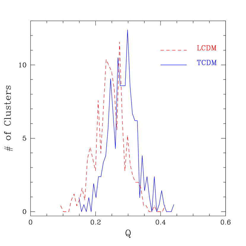
Figure 1.— Histogram of the distribution of the quadrupoles for the whole set of clusters more massive than $4.2\times 10^{14}M_{\odot}$ (On the vertical axis we simply plot the number of clusters above threshold in each bin). TCDM clusters have systematically larger quadrupoles than their $\Lambda$CDM counterparts.

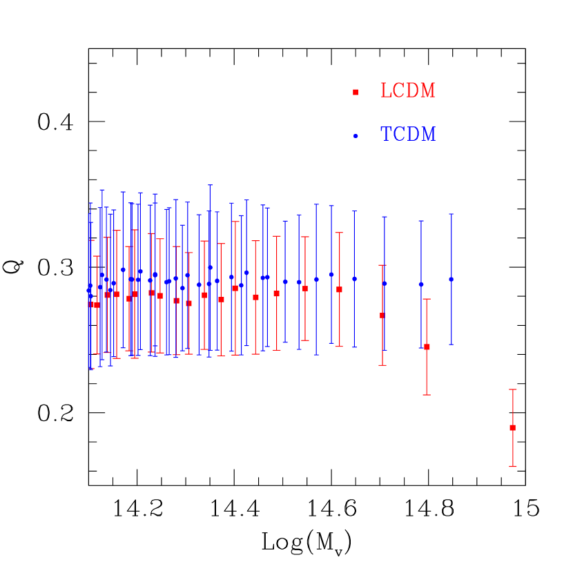
Figure 2.— Average $Q$ vs. virial mass $M_{vir}$. The value of $Q$ is obtained ranging the clusters in order of increasing masses and averaging over 100 neighbours (i.e. they are binned into bins containing 100 clusters each): the value $M_{vir}$ reported is the average of the 100 values.

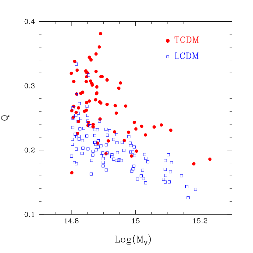
Figure 3.— Scatter plot of $Q$ vs. $M_{vir}$ for rich clusters.

The average quadrupoles of TCDM and $\Lambda$CDM clusters are sistematically different at all masses; the most interesting result however is the strong difference found at the high mass end. Note that this effect could not be detected by WCF96, because of the small number of simulated clusters in their analysis and, most importantly, because they built a sample of essentially equal mass clusters (they rescaled the particle masses of their runs so as to obtain same mass objects). Figure 5 is a scatter plot of $Q$ vs $M_{vir}$ for clusters more massive than $6.3\cdot 10^{14}M_{\odot}$, the mass threshold for which the average quadrupoles of TCDM and $\Lambda$CDM clusters start differing by several percentual points (this threshold yields 105 clusters for $\Lambda$CDM and 81 for TCDM).

How significant is the difference between the two distributions ? Could it be detected through observations of real clusters ? Observations of clusters have made impressive progress in the past decade. As we have reviewed in the Introduction, maps of the mass distribution itself reconstructed from observations of gravitational lensing effects can be systematically built. On the observational side, much progress is a consequence of the development of large–format CCD cameras which can cover fields of $\sim 0.5$ degrees on a side on 4–meter class telescopes. On the theoretical side, different inversion algorithms have been developed to systematically exploit the data on weak gravitational shear, accounting for the effects of realistic PSFs and optimally weighing background galaxies (see the recent reviews by Mellier, 1999, and Bartelmann & Schneider, 2000). Compilations of existing data would allow samples of $\sim 40$ clusters to be examined (e.g. Mellier 2000). However, such samples are hardly homogeneous and the analysis of them would require a careful examination of systematic effects. Only very recently an effort to perform a weak lensing study of a large well defined sample has been started using the NOT and the University of Hawaii 2.24-m telescope (Dahle 2000). On the contrary, inspecting a few very massive clusters is a relatively easy task. This is particularly welcome for the purposes of the present analysis, given that the most prominent differences between the models appear at the high mass end. Let us focus on the behaviour of, say, the first 15 most massive clusters in both samples. As seen in Figure 5 TCDM clusters are clearly shifted towards high values of $Q$.

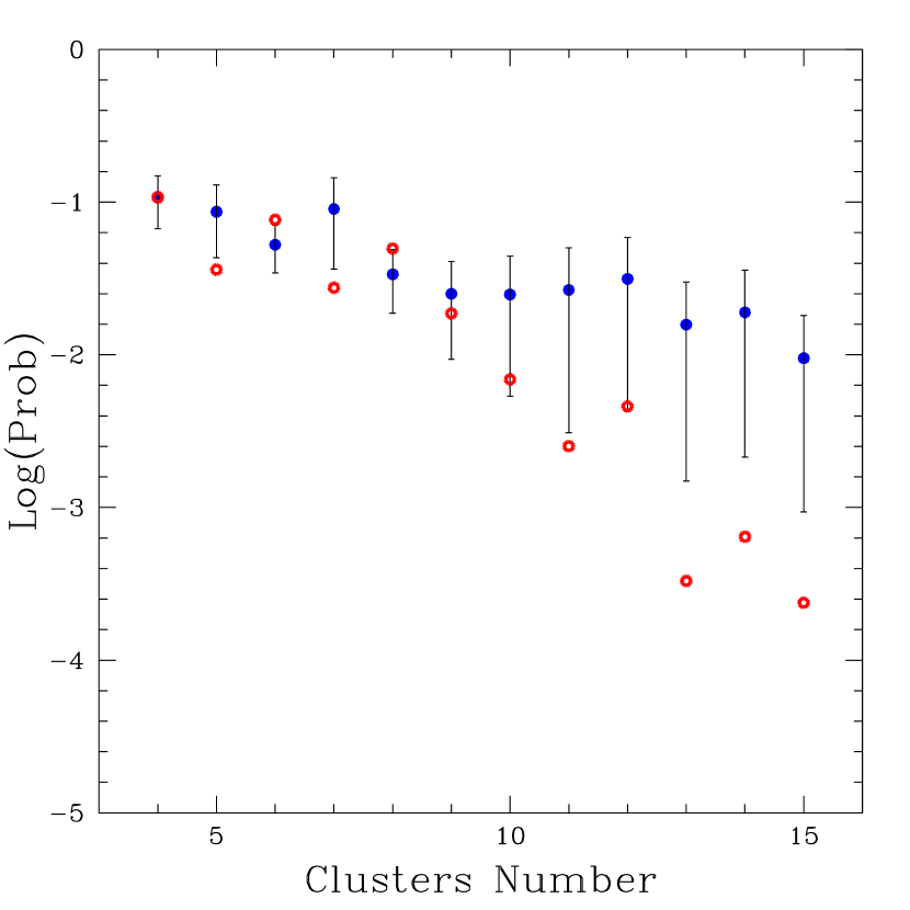
Figure 4.— Kolmogorov-Smirnov probability that the $Q$ measured for the $N$ most massive clusters in the simulation volumes are drawn from the same theoretical distribution. The (red) dots without errorbars refer to clusters selected in the whole simulation boxes ($360\,h^{-1}{\rm Mpc}$ a side). The (blue) dots with errorbars are averages over the results obtained for (eight) half–size subboxes ($180\,h^{-1}{\rm Mpc}$ a side); the errobars correspond to one standard deviation.

In order to quantify the significance of this difference, we perform a K-S test on the distribution of the quadrupoles. Figure 5 gives the probability that the $Q$ measured for the $N$ most massive clusters in $\Lambda$CDM and TCDM are drawn from the same underlying distribution (red dots, without errorbars). The cluster number $N$ is varied between 4 and 15. Even with only 10 clusters the probability that the difference between the $Q$ measured for the $\Lambda$CDM clusters and their TCDM counterparts is just a statistical fluke is below 1%; using 15 clusters, it is well below $1/1000$. Extending the analysis to all the clusters more massive than $6.3\cdot 10^{14}M_{\odot}$ (about twice the mass of the Virgo cluster) yields a KS probability of a mere $10^{-32}$.

The simulated clusters live in a cubic volume of $360\,h^{-1}{\rm Mpc}$ a side. According to the result above, picking $\sim 10$ massive clusters ($M_{vir}\sim 10^{15}M_{\odot}$) in such a volume is sufficient to discriminate between the two models at the 1% confidence limit. Of course, the result will depend on the volume explored, both because $10^{15}M_{\odot}$ clusters are rare objects and because of cosmic variance. Ideally, different simulations would be welcome to thouroughly examine this issue. As a tentative test, we have divided the simulation boxes in eight subboxes of $180\,h^{-1}{\rm Mpc}$ a side; for each pair of corresponding $\Lambda$CDM and TCDM subboxes, we have then repeated the same analyses as for the parent boxes, i.e. we have selected the 15 most massive clusters and estimated the KS probabilities that their $Q$ distributions are drawn from the same underlying model. The results are shown in figure 5 as blue dots with errorbars (1–$\sigma$). The average KS probability increases markedly; however the result is dominated by the outcome of the KS analysis in one of the subboxes, in which the most massive clusters have very similar distributions, whereas in the other subboxes the KS test yields probabilities only slighlty higher than for the whole box. This indicates that at least a volume $\raise-4.0pt\hbox{\hbox to0.0pt{\hbox{$\sim$}\hss}\raise 5.0pt\hbox{$>$}\ }200\,h^{-1}{\rm Mpc}$ is necessary to obtain robust quadrupole statistics able to discriminate between the two cosmologies just using a few tens of massive clusters. A set of large volume simulations would be welcome to examine this issue further.

6. Discussion and Conclusions

Let us first summarize the analyses reported in this paper. We have used two large volume simulations of a $\Lambda$CDM and a TCDM universe, which were started from the same initial random numbers so that the structure forming in each of them are directly comparable. The simulations span a cubic volume of $360\,{\rm Mpc}$ a side. The numerical parameters of the simulations and the linear features of the cosmological models are examined in § 2.

In each simulated volume we have identified the massive virialized systems that would correspond (in mass) to observed galaxy clusters. We have then measured the quadrupole $Q$ of the projected mass distribution of each simulated cluster (we extend our analysis to objects more massive than a threshold $=\,4\times 10^{14}M_{\odot}$).

Studying the statistics of the quadrupoles, we have obtained the following results:

• The distributions of the quadrupoles of TCDM and $\Lambda$CDM clusters differ significantly, with TCDM clusters having systematically larger quadrupoles in agreement with the linear theory expectation that in a high density universe clusters keep accreting material till the present epoch while in a low density universe late accretion and mergers are suppressed. This confirms previous numerical results by Evrard et al.(1993) Mohr et al.(1995) and Wilson, Cole & Frenk (1996b).

• At variance with the previous authors which focussed on a small set of (at that time) high resolution simulations, we have built catalogs of simulated clusters. This allows us to study the dependence of the quadrupoles on cluster mass. We find that the trends of $Q$ vs. $M_{vir}$ of the two models are markedly different at the high mass end. For $M_{vir}\raise-4.0pt\hbox{\hbox to0.0pt{\hbox{$\sim$}\hss}\raise 5.0pt\hbox{$>$}\ }8\cdot 10^{14}M_{\odot}$ (about twice the mass of the Virgo cluster), the average quadrupoles of $\Lambda$CDM clusters drop to values 30% lower than those of their TCDM counterparts of similar mass.

• We have examined how many massive clusters are needed to significatly distinguish between the quadrupole distributions of TCDM and $\Lambda$CDM clusters performing a KS test. We find that, using just the 10 most massive clusters of the samples ($\raise-4.0pt\hbox{\hbox to0.0pt{\hbox{$\sim$}\hss}\raise 5.0pt\hbox{$>$}\ }10^{15}M_{\odot}$ in the simulation volume of $360\,h^{-1}{\rm Mpc}$ a side), the probability that the $Q$ measured are drawn from the same model distribution is less than 1%, and decreases to well below $1/1000$ if the 15 most massive clusters are employed.

• The significance of the test depends on the volume span by the cluster sample and on the number of most–massive clusters which can be taken into account. If such number is restricted to $\cal O$(10), we estimate that a volume $\raise-4.0pt\hbox{\hbox to0.0pt{\hbox{$\sim$}\hss}\raise 5.0pt\hbox{$>$}\ }200\,h^{-1}{\rm Mpc}$ is necessary to obtain robust quadrupole statistics able to discriminate between the two cosmologies. Of course, increasing the number of clusters (that is lowering the mass/richness threshold for a cluster to be considered) implies more and more careful observational work. It should also be noted that, if the mass threshold is pushed down to $\raise-2.0pt\hbox{\hbox to0.0pt{\hbox{$\sim$}\hss}\raise 5.0pt\hbox{$<$}\ }4\times 10^{14}{h^{-1}M_{\odot}}$, no substantial advantage would result from adding more clusters to the sample, as, at such masses, the signal tends to quickly fade. For example, in a box with side $\sim 180\,h^{-1}$Mpc, we find $\sim 25$ clusters above such threshold. In a volume $\sim 10^{7}$–$10^{8}h^{-3}$Mpc³, of the order of what is observationally inspected, the number of significant clusters approaches a total of $\sim 200$. A set of new simulations could be used to determine how effectively different values of $\Lambda$ can be discriminated, should this whole sample of potential data be exploited. From our analysis, we speculate that it could allow us to go beyond discriminating between $\Lambda=0$ and $\Lambda\neq 0$.

These results confirm that the statistics of cluster quadrupoles is sensitive to the cosmological model. In particular this statistics could do more than distinguishing between the currently popular $\Lambda$CDM model and a standard CDM cosmology with zero cosmological constant. Even in the era of high precision cosmology that CMB observations will be hopefully opening soon, the statistical analysis presented here might be quite significant. First of all, it conveys information coming from our own or nearby epochs, allowing a self consistency test of theories tuned at the matter–radiation decoupling epoch. Furthermore, in the case of complex models of dark energy as discussed in the Introduction, it can complement CMB observations, helping to remove residual degenerations in the determination of the cosmological parameters. Of course, using quadrupole statistics requires, from the observational point of view, a strong systematic effort to expand the available data set on weak lensing from galaxy clusters, and, from the theoretical side, a careful examination of the biases affecting the quadrupole estimates of real clusters and their selection (e.g. due to projection effects or the limitations of cluster identification and mass reconstruction algorithms; see e.g. Wilson, Cole & Frenk 1996a and Reblinsky & Bartelmann 1999).

	TCDM	$\Lambda$CDM
$\Omega_{m}$	1	0.65
$\Lambda$	0	0.35
$\Omega_{b}\cdot 10^{2}$	6	6
$n$	0.8	1.05
$h$	0.5	0.65
$Q_{PS,rms}/\mu$K	15.6	20.05
$\sigma_{8}$	0.55	1.08
$\Gamma$	0.32	0.19
$N_{cl}$ (PS; $\delta_{c}=1.69$)	4.2	4.2

Table 1 Parameters of the models. All parameters listed are either input parameters or quantities worked out from the linear theory (see [23]). The normalization to COBE quadrupole was deliberately kept at the $\sim 3\,\sigma$ lower limit, in order to leave some room to the contribution of tensor modes, while being consistent with the data. The expected interval for $N_{cl}$ is 4–6.

References

- [1] Balbi, A. et al.2000, ApJLett, in press (preprint astro-ph/0005124)
- [2] Bardelli, S., Pisani, A., Ramella, M., Zucca, E. & Zamorani, G. 1998, MNRAS, 300, 589
- [3] Bartelmann M., Ehlers J. & Schneider P. 1993, A&A, 280, 351
- [4] Bartelmann M. & Schneider P. 1999, Physics Reports, submitted (preprint astro-ph/9912508)
- [5] de Bernardis, P. et al.2000, Nature, 404, 995
- Bird [1994] Bird C. M., 1994, A.J., 107, 1637
- Borgani et al. [1997] Borgani S., Gardini A., Girardi M., Gottlöber S., 1997, NewA, 2, 119
- [8] Brainerd, T. G., Goldberg, D. M. & Villumsen, J. V. 1997, ApJ, 502 505
- [9] Caldwell, R. R., Dave R. & Steinardt, P. J. 1998, Phys. Rev. Lett. 80, 1582
- Cole et. al [1997] Cole S., Weinberg D.H., Frenk C.S., Ratra B., 1997, MNRAS, 289, 37
- [11] Clowe, D., Luppino, G., Kaiser, N. & Gioia, I. 2000, ApJ, submitted (preprint astro-ph/0001356)
- [12] Crooks, J. L., Dunn, J. O., Frampton, P. H., Ng, Y. J. & Rhom, R. M. 2000, (preprint astro-ph/0005406)
- [13] Dahle, H. 2000, preprint (astro-ph/0009393)
- [14] Davis, M., Efstathiou, G., Frenk, C. S. & White, S. D. M. 1985, ApJ, 292, 371
- [15] De Zotti G. et al.2000, Proc. of the Conference: ”3 K Cosmology”, Roma, Italy, 5-10 October 1998, AIP Conference Proc. (preprint astro-ph/9902103)
- Doroshkevich et al. [1980] Doroshkevich A.G., Kotok E.V., Novikov I.D., Polyudov A.N., Shandarin S.F., Sigov Yu.S., 1980, MNRAS, 192, 321
- Dressler & Schectman [1988] Dressler A., Schectman S., 1988, A.J., 95, 284
- Efstathiou et al. [1985] Efstathiou G., Davis M., Frenk C.S., White S.D.M., 1985, ApJS, 57, 241
- Eke, Cole Frenk [1996] Eke V.R., Cole S., Frenk C.S., 1996, MNRAS, 282, 263
- Eke, Cole, Frenk Henry [1998] Eke V.R., Cole S., Frenk C.S., Henry J.P., 1998, MNRAS, 298, 1145
- Evrard et al. [1994] Evrard A. E., Mohr J. J., Fabricant D. G., Geller M. J., 1994, Ap.J.L., 419, L9
- Forman & Jones [1990] Forman W. F., Jones C. J., 1990, in Oegerle W. R., Fitchett M. J., Danly L., ed, Clusters of Galaxies. Cambridge University Press, p. 257
- Gardini et al. [1999] Gardini A., Murante G. Bonometto S. A., 1999, ApJ, 524, 510
- Geller & Beers [1982] Geller M. J., Beers T. C., 1982, P.A.S.P., 94, 421
- [25] Ghigna, S., Moore, B., Governato, F., Lake, G., Quinn, T. & Stadel, J. 1998, MNRAS, 300, 146.
- Girardi et al. [1998] Girardi M., Borgani S., Giuricin G., Mardirossian F., Mezzetti M., 1998, ApJ, 506, 45
- Governato et al. [1999] Governato F., Babul A., Quinn T., Tozzi P., Baugh C.M., Katz N., Lake G., 1999, MNRAS, 307, 949
- [28] Graham, P. S., Kneib, J.-P., Ebeling, H., Czoske, O. & Smail, I. 2000, ApJ, submitted (preprint astro-ph/0008315)
- [29] Hattori, M., Kneib, J.-P. & Makino, N. 1999, Progress of Theoretical Physics, in press (preprint astro-ph/9905009)
- [30] Hanany, S. et al.2000, ApJLett, submitted (preprint astro-ph/0005123)
- Hockney Eastwood [1981] Hockney R.W., Eastwood J.W., 1981, Computer Simulation Using Particles, McGraw–Hill, New York
- [32] Jaffe, A. H. et al.2000, Phys. Rev. Lett., submitted (preprint astro-ph/0007333)
- Jungman et al. [1996] Jungman G., Kamionkowski M., Kosowsky, A. & Spergel D. N. 1996, Phys. Rev. Lett. 76, 1007
- [34] Kaiser, N. & Squires, G. 1993, ApJ, 404, 441
- [35] Kaiser, N. 1999, Review talk at Boston 99 lensing meeting, (preprint astro-ph/9912569
- [36] Klypin, A., Gottlöber, S., Kravtsov, A. & Khokhlov, M. 1999, ApJ, 516, 530
- Kamionkowski & Kosowsky [1999] Kamionkowski M. & Kosowsky A. 1999, Ann.Rev.Nucl.Part.Sci. 49, 77
- [38] Lange, A. E. et al.2000, Phys. Rev. D, submitted (preprint astro-ph/0005018)
- Lacey & Cole [1993] Lacey C., Cole S., 1993, M.N.R.A.S., 262, 627
- Mellier [1999] Mellier, Y. 1999, ARA&A, 37, 127
- Mo, Jing White [1996] Mo H.J., Jing Y.P., White S.D.M., 1996, MNRAS, 282, 1096
- Mohr et al. [1995] Mohr J. J., Evrard A. E., Fabricant D. G., Geller M. J., 1995, Ap.J., 447, 8
- [43] Moore, B., Governato, F., Quinn, T., Stadel, J. & Lake, G. 1998, ApJ, 499, 5
- [44] Okamoto, T & Habe, A. 1999, ApJ, 516, 591
- [45] Page L. 2000, Proc IAU Symposium 201, Eds. Lasenby A. & Wilkinson A. (preprint astro-ph/0012214)
- Peebles [1980] Peebles P.J.E., 1980, The Large Scale Structure of the Universe, Princeton University Press, Princeton
- Perlmutter et al. [1998] Perlmutter S., et al., 1998, Nature, 391, 51
- Postman [1998] Postman M., Cluster as Tracers of the Large Scale Structure, in Evolution of Large-Scale Structure: From Recombination to Garching: Proc. MPA/ESO Cosmology Conference, Garching, Germany, August 1998, preprint astro–ph/9810088
- [49] Reblinsky K. & Bartelmann M. 1999, A&A, 345, 1
- Richstone et al. [1992] Richstone D., Loeb A., Turner E. L., 1992, Ap.J., 393, 477
- Riess et al. [1998] Riess A.G., et al., 1998, AJ, 116, 1009
- [52] Seitz, C. & Schneider, P. 1995, A&A, 297, 287
- [53] Solanes, J. M., Salvador-Solé, E., González–Casado, G. 1999, A&A, 343, 733
- [54] Tegmark, M., Zaldarriga, M. & Hamilton A. J. S. 2001, Phys.Rev. D63, 043007
- [55] Tyson, J.A., Valdes, F. & Wrenk, R. 1990, ApJ, 349, L1
- Valdarnini, Ghizzardi Bonometto [1998] Valdarnini R., Ghizzardi S., Bonometto S.A., 1999, New Astr., 4, 71
- Viana Liddle [1996] Viana P.T.P., Liddle A.R., 1996, MNRAS, 281, 323
- West & Bothun [1990] West M. J., Bothun G. D., 1990, Ap.J., 350, 36
- West et al. [1995] West M. J., Jones C., Forman W., 1995, Apj, 451L, 5W
- [60] White, S. D. M. & Rees, M. 1978, MNRAS, 183, 341
- White, Efstathiou Frenk [1993] White S.D.M., Efstathiou G., Frenk C., 1993, MNRAS, 262, 1023
- [62] White, M., Scott, D. & Pierpaoli, E. 2000, ApJ, in press (preprint astro-ph/0004385)
- [63] Wilson, G., Cole, S. & Frenk, C. S. 1996a, MNRAS, 280, 199
- [64] Wilson, G., Cole, S. & Frenk, C. S. 1996b, MNRAS, 282, 501
- [65] Wittman, D, Dell’Antonio, I., Tyson, T., Bernstein, G., Fischer, P. & Smith, D. 2000, preprint (astro-ph/0009362)
- Zel’dovich [1970] Zel’dovich Ya. B., 1970, AA, 5, 84