An Adaptive Grid, Implicit Code for Spherically Symmetric, General Relativistic Hydrodynamics in Comoving Coordinates

Abstract

We describe an implicit general relativistic hydrodynamics code. The evolution equations are formulated in comoving coordinates. A conservative finite differencing of the Einstein equations is outlined and artificial viscosity and numerical diffusion are discussed. The time integration is performed with AGILE, an implicit solver for stiff algebro-differential equations on a dynamical adaptive grid. We extend the adaptive grid technique, known from nonrelativistic hydrodynamics, to the general relativistic application and identify it with the concept of shift vectors in a 3+1 decomposition. The adaptive grid minimizes the number of required computational zones without compromising the resolution in physically important regions. Thus, the computational effort is greatly reduced when the zones are subject to computationally expensive additional processes, such as Boltzmann radiation transport or a nuclear reaction network. We present accurate results in the standard tests for supernova simulations: Sedov’s point blast explosion, the nonrelativistic and relativistic shock tube, the Oppenheimer-Snyder dust collapse, and homologous collapse.

1 Introduction

Consider a physical variable $y$ that evolves in time $t$ according to a differential equation $dy/dt=f(y)$. The simplest implicit finite differencing relates the value of $y^{n}$ at time $t^{n}$ to its previous value $y^{n-1}$ at time $t^{n-1}$ by

$$\frac{y^{n}-y^{n-1}}{t^{n}-t^{n-1}}=f(y^{n}).$$ (1)

This equation can be solved for $y^{n}$ at each time step $n=1\ldots\infty$. Depending on the properties of the function $f$, a computationally expensive solution of a nonlinear algebraic equation is required in most cases. This is not the case with the explicit finite differencing where the evaluation of $f$ is based on the old values $y^{n-1}$. The two discretization variants appear to be similar for small time steps where $|f(y^{n})-f(y^{n-1})|$ is small. However, the behavior dramatically differs for larger steps: If a physical equilibrium with the static solution $0=f(y^{\infty})$ exists, one easily checks with equation (1) that the equilibrium solution can be approached in one large time step because of the bound value of $|y^{\infty}-y^{n-1}|$. Explicit finite differencing, on the other hand, does not lead to a physically meaningful solution with time steps larger than a characteristic time scale that is determined by the function $f$. Implicit methods guarantee smooth transitions between dynamical phases and equilibrium phases. On a long time scale, they automatically adjust the equilibrium to exterior dependencies and provide an averaging approximation where physical oscillations around the equilibrium are not of primary interest. Although implicit schemes certainly are capable of tracking the full dynamical solution on short time scales, a calculation with time steps smaller than the characteristic time scale is much more efficiently done with explicit finite differencing. The reduction in the number of time steps with the implicit technique has to compensate the additional effort invested with the solution of the algebraic equations.

Processes in astrophysics involve characteristic time scales that differ by orders of magnitude. For example Henyey et al. (1959) had to introduce implicit finite differencing in stellar evolution calculations, where nuclear reactions as well as hydrodynamics were assumed to be quasi-static on the time scale of stellar evolution. The system of algebraic equations is traditionally solved with a Newton-Raphson scheme. The numerical effort increases steeply with the number of unknowns that have to be determined in one time step. Thus, implicit approaches are predestined for systems of moderate size where the evolution time scale is comparable to the time scale of the underlying physical processes somewhere in space or time, and exceeds the latter by far elsewhere or at another time. Because of this size restriction, implicit hydrodynamics has mainly been applied in one-dimensional systems, such as in spherically symmetric hydrodynamics codes for supernova simulations (Schinder & Bludman, 1989; Swesty, 1995; Yamada, 1997). Spherical symmetry additionally allows the use of Lagrangian comoving coordinates and a full treatment of general relativity (Misner & Sharp, 1964). The evolution of the metric can be included self-consistently into the solution for the nonlinear algebraic equations that emerge from the implicit finite differencing.

Fig. (1) shows the connection between several technical features that go along with a hydrodynamics code that is based on implicit finite differencing. Eggleton (1971) used an adaptive grid in his quasistatic stellar evolution code. Together with the hydrostatic equations, a grid equation is solved that determines where a fixed number of grid points is located to optimally sample the profile of the star. A dynamical adaptive grid was suggested by (Harten & Hyman, 1983) and the formulation of radiation hydrodynamics on a dynamical adaptive grid was provided by Winkler, Norman, & Mihalas (1984) and implemented in Newtonian (Winkler & Norman, 1986) and special relativistic (Norman & Winkler, 1986) hydrodynamics. Dorfi & Drury (1987) found a simple and robust implicit prescription to guide the dynamics of the adaptive grid according to the evolution of the physical state. Note the difference between the dynamical adaptive grid where a fixed number of grid points continously moves through the computational domain and a static adaptive grid where static grid points are inserted or removed according to resolution requirements. The dynamical adaptive grid technique found applications in astrophysical high-resolution calculations (Dorfi & Gautschi, 1989; Mair, 1990), and a well documented implementation of the dynamical adaptive grid technique for Newtonian hydrodynamics with radiative transfer in different one-dimensional geometries has been provided by Gehmeyr & Mihalas (1994) in the code TITAN.

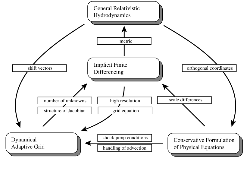
Figure 1: The interdependence between general relativity, implicit finite differencing, conservative equations, and the dynamical adaptive grid in spherically symmetric hydrodynamics.

We resume the description of Fig. (1) with the relationship between a dynamical adaptive grid and implicit hydrodynamics. The solver of the algebraic equations easily incorporates the solution of the implicit grid equation. The zones are dynamically concentrated in the regions of action or where a high resolution is required. This assures that most of the zones actively contribute to the interesting part of the evolution and do not clump together in regions of well-known physical equilibrium. The dynamical adaptive grid can reduce the required number of grid points by orders of magnitude with respect to an equidistant grid, and the implicit scheme greatly benefits from this size reduction in the solution vector. Since the dynamical grid changes neither the total number of grid points nor its ordering, the structure of the Jacobian that has to be inverted in the Newton-Raphson scheme remains unchanged during the simulation. Furthermore, the high resolution achieved with the adaptive grid is only advantageous in combination with implicit hydrodynamics because the Courant-Friedrichs-Lewy condition (Courant, Friedrichs, & Lewy, 1928) would impose severe restrictions on the maximum time step in explicit schemes.

Of course, the adaptive grid also comes with difficulties. The moving grid relates different spatial points in the physical state vector across one and the same time step. This requires a proper handling of advection in the formulation of the physical equations on the adaptive grid. Moreover, the advection introduces extended coupling between neighboring zones and therewith increases the density of the Jacobian in the Newton-Raphson scheme. A conservative formulation of the physical equation provides a solid basis for the discretization of the advection. Conserved quantities are transfered from one zone into a neighboring zone. A formulation of the dynamics in terms of conservation laws has additional benefits: (i) Fundamental conservation laws are also valid at discontinuities and allow an accurate numerical solution - e.g., for the propagation of shock waves. This is not the case with arbitrary finite difference approximations. (ii) The integration of a conserved quantity over adjacent fluid elements does not depend on the fluxes at the enclosed boundaries. Thus, discretization errors have mainly local influence. This advantage is important for the implicit solution of problems involving scale differences of many orders of magnitude. (iii) The integration over the whole computational domain of the single-fluid-element conservation laws leads to the total conservation of fundamental physical quantities, independent of the resolution in the conservative finite difference representation. These contributions of a conservative formulation to the adaptive grid and implicit solution are also drawn in Fig. (1).

In this paper, we describe our implementation of the dynamical adaptive grid technique in general relativistic hydrodynamics. The dynamical adaptive grid is nothing other than a continuous and time dependent shift in the coordinates with respect to Lagrangian or Eulerian coordinates. This freedom of coordinate choice has long been explored in the general relativistic case, where in addition to the time slices, shift vectors have to be defined in a 3+1 decomposition (Arnowitt, Deser, & Misner, 1962; Smarr & York, 1978). There is no difference between a dynamical adaptive grid and a specific choice of shift vectors in the general relativistic description. However, as far as the numerics is concerned, the formulation with shift vectors only provides a set of analytical equations, while the Newtonian adaptive grid technique can be generalized to a detailed prescription for a stable numerical implementation of shift vectors in the general relativistic case. Thus, instead of directly applying a discretization of appropriate shift vectors, we first search for a conservative formulation of hydrodynamics in Lagrangian coordinates and then apply the generalized adaptive grid technique to implement the shift vectors that lead to an optimal resolution of the physical state at important locations.

All the features drawn in Fig. (1) come together in an important astrophysical application: core collapse supernovae. The compact object at the center of the star requires a general relativistic treatment (Bruenn, DeNisco, & Mezzacappa, 2001; Liebendörfer et al., 2001). The time scales of radiation transport, hydrodynamics, and neutrino diffusion differ by orders of magnitude and call for implicit techniques. The computational domain covers densities from $10^{5}$ g cm^-3 in the outer layers of the calculational domain to several times $10^{14}$ g cm^-3 in central regions of the proto-neutron star. At these higher-than-nuclear densities the stiffness of the equation of state is responsible for very short hydrodynamical time scales. The speed of sound waves reaches several 10% of the velocity of light. If one is not interested in the ringing of the neutron star, this time scale is prohibitive for the calculation of the long term physics in the outer range with schemes implementing explicit finite differencing. The supernova shock formed after stellar core collapse and bounce requires reasonable resolution. Moreover, in the case of a supernova explosion, the adaptive grid allows a smooth propagation of the shock through the outer layers; and in the case of black hole formation, a robust implementation of shift vectors might help to shift the arising coordinate singularity at the Schwarzschild horizon out of the computational domain (Liebendörfer & Thielemann, 2000). Even the conservative formulation of the hydrodynamic equations is physically motivated: A meticulous energy conservation in the finite difference scheme is required to allow statements on the success of a supernova explosion (Mezzacappa et al., 2001). The balance of gravitational, internal, and neutrino energy is two orders of magnitude smaller than the individual constituents. The total energy is then comparable to the explosion energy, i.e. about one percent of the energy stored in the neutrino field. The bookkeeping of this energy has to be based on a careful implementation of the mutual energy and momentum transfer between the neutrino radiation field and the matter. For the determination of the explosion energy to an accuracy of at least one order of magnitude, one may tolerate an energy drift of not exceeding a fraction of $10^{-3}$ of the internal, gravitational or neutrino radiation energy. This drift extends over the whole calculation time of more than $10000$ time steps, so that systematic deviations of energy conservation may not exceed a fraction of $10^{-7}$ per time step. On current computer hardware, it is not yet possible to simulate in multi-dimensional general relativity the confluence of accurate multigroup neutrino transport, high resolution hydrodynamics, magnetic fields, and up-to-date nuclear physics input. The complexity of supernova explosions is best explored in separate restricted investigations. Spherically symmetric simulations are able to incorporate the best available neutrino transport techniques (Rampp & Janka, 2000; Mezzacappa et al., 2001) in self-consistent simulations with high resolution and allow the detailed study of high density weak interactions and nuclear physics.

In the following section, we write down conservative equations of general relativistic hydrodynamics in spherical symmetry and discuss the relation between shift vectors and the adaptive grid. The adaptive grid technique of Winkler, Norman, & Mihalas (1984) is extended to general relativity and applied in combination with the grid equation of Dorfi & Drury (1987). We then proceed with a description of our approach to automatically and implicitly integrate a system of stiff ordinary differential equations in time and outline the spatially staggered finite differencing of the physical equations. Numerical diffusion and artificial viscosity are discussed. In section 4 we run the standard supernova test simulations with our code, AGILE, and compare the results to analytical solutions and the Piecewise Parabolic Method (PPM) (Colella & Woodward, 1984).

2 Conservative Equations on the Dynamical Adaptive Grid

2.1 Relativistic hydrodynamics in spherical symmetry

General relativistic four-dimensional space-time can be described in terms of consecutive three-dimensional time slices (Arnowitt, Deser, & Misner, 1962). The definition of the time slices and the choice of coordinates within the slices is not given by the dynamics of the matter; it has to be imposed from the outside as a part of the description. The time slices comprise the events that are made simultaneous with respect to coordinate time. They are defined by a lapse function that describes the proper time lapse to the infinitesimally close neighbor time slice $t+\delta t$ along a path orthogonal to the time slice at time $t$. The three-dimensional coordinates within a time slice are then specified by a shift vector function describing the spatial shift of points with the same coordinate label between infinitesimally close neighbor slices. Reference for the shift is again the path orthogonal to the slice (Smarr & York, 1978).

In Newtonian hydrodynamics, time and space are understood as separate entities. Only one definition of the time slices is possible: orthogonal to the time axis. However, a free choice of coordinates within the time slices persists. We may choose Eulerian coordinates along the time axis or Lagrangian coordinates along fluid element trajectories. If one understands the grid point labels in a dynamical adaptive grid technique as coordinates, many mappings between such coordinates and the location of fluid elements can be realized with appropriate prescriptions for the motion of the adaptive grid. These choices are easily interpreted in the general relativistic view: The Eulerian coordinates correspond to vanishing shift vectors and the Lagrangian coordinates correspond to shift vectors equal to the three-velocity of fluid elements. In the adaptive grid case, the shift vectors are identified with the grid velocity.

In the following investigation, the time slices are chosen orthogonal to matter trajectories such as to produce comoving coordinates with vanishing shift vectors. Nevertheless, the relationship between adaptive grids in Newtonian space-time and shift vectors in the general relativistic context provides a guideline for the implementation of shift vectors in general relativistic simulations. Fixed coordinate intervals can be mapped to the time slices at will in order to resolve physically interesting regions with high precision.

We start with the spherically symmetric Einstein equations in comoving orthogonal coordinates as given by Misner & Sharp (1964). They are based on the metric

$$ds^{2}=-\alpha^{2}dt^{2}+\left(\frac{r^{\prime}}{\Gamma}\right)^{2}da^{2}+r^{2}\left(d\vartheta^{2}+\sin^{2}\vartheta d\varphi^{2}\right),$$ (2)

where $r$ is the areal radius and $a$ is a label corresponding to an enclosed rest mass (the prime denotes a derivative with respect to $a$: $r^{\prime}=\partial r/\partial a$). The proper time lapse of an observer attached to the motion of rest mass is related to the coordinate time $dt$ by the lapse function $\alpha$. The angles $\vartheta$ and $\varphi$ describe a two-sphere.

The thermodynamic state of a fluid element is given in its rest frame by the rest mass density, $\rho$, the temperature, $T$, and, in our application, the electron fraction $Y_{e}$. An equation of state renders the composition in nuclear statistical equilibrium, the specific internal energy, $e$, and the isotropic pressure $p$. In analogy to the definitions of Romero et al. (1996) in polar slicing and radial gauge, we compose conserved quantities for specific volume, total energy, and radial momentum:

$$\frac{1}{D} = \frac{\Gamma}{\rho}$$ (3)

$$\tau = \Gamma e+\frac{2}{\Gamma+1}\left(\frac{1}{2}u^{2}-\frac{m}{r}\right)$$ (4)

$$S = u\left(1+e\right).$$ (5)

The velocity $u$ is equivalent to the $r\,$-component of the fluid four-velocity as observed from a frame at constant areal radius (May & White, 1967). In the special relativistic limit, $\Gamma=\sqrt{1+u^{2}-2m/r}$ becomes the Lorentz factor that takes the boost between the inertial and the comoving observers into account. The gravitational mass $m$ is the total energy enclosed in the sphere at rest mass $a$. In the nonrelativistic limit, we retrieve with $\alpha=\Gamma=1$ the familiar specific volume $1/D=1/\rho$, the sum of the specific internal, kinetic, and gravitational energy $\tau=e+u^{2}/2-m/r$, and the specific radial momentum $S=u$.

With these definitions, the complete system of general relativistic hydrodynamics equations can be written in a conservative form (Liebendörfer, Mezzacappa, & Thielemann, 2001):

$$\frac{\partial}{\partial t}\left[\frac{1}{D}\right] = \frac{\partial}{\partial a}\left[4\pi r^{2}\alpha u\right]$$ (6)

$$\frac{\partial\tau}{\partial t} = -\frac{\partial}{\partial a}\left[4\pi r^{2}\alpha up\right]$$ (7)

$$\frac{\partial S}{\partial t} = -\frac{\partial}{\partial a}\left[4\pi r^{2}\alpha\Gamma p\right]$$ (8)

$$- \frac{\alpha}{r}\left[\left(1+e+\frac{3p}{\rho}\right)\frac{m}{r}+8\pi r^{2}\left(1+e\right)p-\frac{2p}{\rho}\right]$$

$$\frac{\partial V}{\partial a} = \frac{1}{D}$$ (9)

$$\frac{\partial m}{\partial a} = 1+\tau$$ (10)

$$0 = \left(1+e\right)\frac{\partial\alpha}{\partial a}+\frac{1}{\rho}\frac{\partial}{\partial a}\left[\alpha p\right].$$ (11)

Equations (6)-(8) describe the conservation of volume (analogously to mass conservation in Eulerian coordinates), total energy, and radial momentum respectively. The constraints (9) and (10) explain themselves in the analogy to the Newtonian limit, where the first becomes the definition of the rest mass density and the second the Poisson equation for the gravitational potential. The enclosed volume in Eq. (9) is defined by the areal radius as in the Newtonian limit, $V=4\pi r^{3}/3$. The condition for the lapse function in equation (11) is derived from the space-space components of the Einstein field equations.

2.2 Shift vectors and the dynamical adaptive grid

In Fig. (1) we have now moved from the equations of general relativistic hydrodynamics to their conservative formulation in specific coordinates as shown in the lower right corner. In order to traverse to the left towards a stable implementation of the adaptive grid, we rewrite the derivations of Winkler, Norman, & Mihalas (1984) in a form that applies to the general relativistic case as well. The goal is a stable and conservative finite difference representation of equations (6)-(8) in terms of $n$ grid points, $(a_{i}(t),i=1\ldots n)$, that continuously move with respect to the enclosed rest mass label.

We concentrate on observers at rest in their slice. They reside in local orthogonal reference frames that we assume to be collinear with global coordinates $A$. Consequently, coordinates $A$ have vanishing shift vectors everywhere. We introduce another system of global coordinates, $B$, having arbitrary shift vectors on the same time slices. Let us select a fixed grid in coordinates $B$: $\{\vec{q}_{i\in{\rm N}^{3}}\in{\rm R}^{3},i_{1}=1\ldots n_{1},i_{2}=1\ldots n_{2},i_{3}=1\ldots n_{3}\}$. The trace of the world-lines along this grid defines a moving grid in coordinate system $A$: $\{\vec{a}(t,\vec{q}_{i})\}$. The grid world lines along coordinate system $B$ cut the continuum into zones $\Delta q$ on each time slice. These zones contain a time dependent selection of observers in coordinate system $A$: $\Delta a=\{\vec{a}(t,\vec{q}),\vec{q}\in\Delta q\}$. Based on the observations $y$ of single observers $\vec{a}$ in the zone, we define a zone integral of the observations

$$\langle y(t,\vec{a})\rangle=\int_{\Delta a}y(t,\vec{a})d\vec{a}.$$ (12)

In coordinate system $A$, the borders of the zones change with time according to the shift vectors in coordinate system $B$. In Newtonian parlance, one can identify the moving zones in coordinate system $A$ with the motion of an adaptive grid. The important point is that the adaptive grid only regroups the observers into new zones. As stated already by Winkler, Norman, & Mihalas (1984), the adaptive grid never changes the reference frame of the observations. It solely determines the zonewise support for the integration of the observations in the time slice.

In order to formulate time evolution equations, we are interested in the temporal change of the zone-integrated quantity

$$\langle y(t,\vec{q})\rangle=\int_{\Delta a}y(t,\vec{a})d\vec{a}$$ (13)

in a specific zone $\Delta q$. We can apply the Reynolds theorem to relate the time derivative $\partial\langle y(t,\vec{q})\rangle/\partial t$ in coordinate system $B$ to the time derivative $\langle\partial y(t,\vec{a})/\partial t\rangle$ in coordinate system $A$:

$$\frac{\partial\langle y(t,\vec{q})\rangle}{\partial t}=\left<\frac{\partial y(t,\vec{a})}{\partial t}\right>+\int_{\partial(\Delta a)}y(t,\vec{a})\left(\frac{\partial\vec{a}(t,q)}{\partial t}\cdot\vec{n}\right)dS.$$ (14)

Note that the Reynolds-theorem is a mathematical relation that has no physical content. The left hand term is the temporal change in the zone average of $y$ in the numerically accessible coordinate system $B$. The first term on the right hand side relates this time derivative to the time derivative in orthogonal coordinates $A$ that is easily evaluated based on the physical equations describing the time evolution. The correction in the second term on the right hand side is due to the grid motion. It is an integral over the zone surface elements $dS$ (with normal $\vec{n}$) that corrects for the observations made by observers that enter or leave the zone during grid motion.

If an equation describing the physical evolution is written in a conservative form

$$\left<\frac{\partial y(t,\vec{a})}{\partial t}\right>+\int_{\partial(\Delta a)}\left(\vec{f}(t,\vec{a})\cdot\vec{n}\right)dS=\int_{\Delta a}s(t,\vec{a})d\vec{a}$$ (15)

with a source $s(t,\vec{a})$, its formulation on the adaptive grid simply becomes

$$\frac{\partial\langle y(t,\vec{q})\rangle}{\partial t}+\int_{\partial(\Delta a)}\left(\left[\vec{f}(t,\vec{a})-y(t,\vec{a})\frac{\partial\vec{a}(t,\vec{q})}{\partial t}\right]\cdot\vec{n}\right)dS=\int_{\Delta a}s(t,\vec{a})d\vec{a}.$$ (16)

The motion of zone boundaries naturally leads to a flux entering or leaving the zone. The rate of coordinate change at a fixed grid point $v^{\rm rel}=-\frac{\partial\vec{a}(t,\vec{q})}{\partial t}$ defines a “grid velocity” with respect to coordinates $A$. In our spherically symmetric case, the Reynolds theorem reduces to

$$\frac{\partial}{\partial t}\int_{a(t,q_{i})}^{a(t,q_{i+1})}yda=\int_{a(t,q_{i})}^{a(t,q_{i+1})}\frac{\partial y(t,a)}{\partial t}da+\left[y\frac{\partial a(t,q)}{\partial t}\right]_{a(t,q_{i})}^{a(t,q_{i+1})}$$ (17)

and leads for example to the continuity equation (6) on the adaptive grid

$$\frac{\partial}{\partial t}\int_{a(t,q_{i})}^{a(t,q_{i+1})}\frac{1}{D}da+\left[-4\pi r^{2}\alpha u-\frac{1}{D}\frac{\partial a(t,q)}{\partial t}\right]_{a(t,q_{i})}^{a(t,q_{i+1})}=0.$$ (18)

The integral of the conserved quantity (e.g. volume) over the rest mass of the star only depends on surface terms in this favorable form because contributions from zone interfaces exhibit exact cancellation. Thus, the motion of the adaptive grid affects local resolution but not global conservation.

2.3 Dynamics of the adaptive grid

After having described the formulation of physical equations on an adaptive grid, we focus on the independent question, how to adapt the grid to interesting features in the physical evolution. The basic idea is not only to resolve steep gradients with a locally increased grid point concentration. To a certain extent, the dynamical adaptive grid is also capable to capture a self-similar flow and propagate it through the computational domain mainly by grid motion instead of rapid changes in the physical state of zones. This can lead to larger time steps when steep gradients are present. For example, if a shock front is smeared out over several grid points, it takes a width $\Delta q$ in grid point labels $q$ (see Fig. (2)).

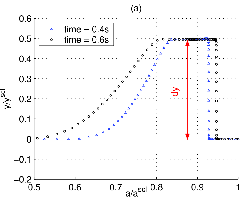
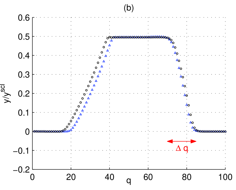
Figure 2: This shock tube simulation (described in section 4.5) illustrates the dynamics of the adaptive grid. Data at two different times are shown. Graph (a) shows the scaled velocity profile in coordinates A, i.e. versus enclosed mass. We indicate the velocity jump across the shock with $dy$. The grid is set to produce equidistant generalized arclength between grid points. This is only qualitatively visible in this graph because of the influence of the other variables and the spatial smoothing operator that guarantees a smooth reduction of the resolution with increasing distance from the shock. Graph (b) shows the same profile in coordinates B, i.e. versus grid label. The shock is smoothly spread over an interval $\Delta q$ that is used to estimate the time step restriction, equation (19). The profile in the computer representation (b) is fairly stationary, while the shock propagation in physical space (a) is dominated by the evolution of the mapping $a(t,q)$.

Suppose the shock moves with velocity $v_{q}$ with respect to the grid; then there is time $\Delta t=\Delta q/v_{q}$ to change the variables from their pre-shock to their post-shock values. We consider the variable $y$ with the largest relative jump $|dy/y|$ at the shock front. If the relative change of the variable per time step is limited to $\varepsilon$ one gets from $|y|+|dy|\leq|y|(1+\varepsilon)^{n}$ about $n=\ln(1+|dy/y|)/\ln(1+\varepsilon)$ time steps for this change. Therefore, the time step is limited by

$$\Delta t<\frac{\Delta q\ln(1+\varepsilon)}{v_{q}\ln(1+|dy/y|)}.$$ (19)

In contrast to Lagrangian or Eulerian schemes, this time limit is not restrictive with the adaptive grid. Firstly, the high resolution at the shock front gives a large $\Delta q$ and secondly, the fact that the grid points tend to move with the shock structure makes the velocity difference between the shock front and the grid, $v_{q}$, very small.

We have implemented the grid equation of Dorfi & Drury (1987). We only differ in one detail: The scheme has been transferred from Eulerian coordinates in flat space to comoving coordinates in Misner-Sharp time slices. Thus, we retrieve a Lagrangian scheme if the adaptive grid is switched off. The grid equation of Dorfi and Drury is based on a resolution function,

$$R(t,a)=\left(1+\sum\left(\frac{a^{{\rm scl}}}{y^{{\rm scl}}}\frac{\partial y(t,a)}{\partial a}\right)^{2}\right)^{\frac{1}{2}},$$ (20)

where the sum includes a selection of relevant variables $y$ as e.g. velocity, density, etc.. We set the global scale in this equation to $y^{\rm scl}=\sum_{i}\left|y_{i+1}-y_{i}\right|$. In terms of a grid point concentration $n=a^{{\rm scl}}(\partial a(t,q)/\partial q)^{-1}$ the grid equation implements the requirement

$$\frac{\partial}{\partial q}\left(\frac{n}{R}\right)=0.$$ (21)

If we imagine the variables $y/y^{{\rm scl}}$ plotted in a graph versus $a/a^{{\rm scl}}$, this condition enforces a constant value of

$$\frac{n}{R}=\left(\left(\frac{\partial a(t,q)}{a^{{\rm scl}}\partial q}\right)^{2}+\sum\left(\frac{\partial y(t,q)}{y^{{\rm scl}}\partial q}\right)^{2}\right)^{-\frac{1}{2}},$$ (22)

equivalent to a constant generalized arc length per grid point interval $\Delta q$. The projection of grid points to the $a/a^{{\rm scl}}$-axis results in an increased grid point concentration at locations with steep gradients in the variables $y/y^{{\rm scl}}$. This basic approach is refined by the sophisticated application of operators for spatial smoothing and temporal retardation of the grid adaption as described by Dorfi & Drury (1987) (see Fig. (2)).

3 Numerical Method

The nonlinear partial differential equations (6)-(8) and the constraints (9)-(11), (21) are finite differenced in the spatial direction to build a large system of coupled ordinary differential equations with algebraic constraints. Each independent variable in each zone acts as an individual unkown function of time in the solution vector. In a second step, this large system of potentially stiff algebro-differential equations is integrated in time with our solver AGILE. Experimentation was necessary to find the final finite difference representation of the hydrodynamical equations. We have therefore separated the solver for the ordinary differential equations and the adaptive grid equation from the modules that describe and discretize the actual physical equations. AGILE has the capapility to calculate the Jacobian of the physical equations automatically for the implicit time evolution. This feature substitutes the cumbersome and errorprone coding of the Jacobian and leaves room for the motivation to change and improve the physical equations.

In the following subsection we start with the description of the time evolution in AGILE. Then, we discuss the numerical diffusion induced by the advection that accompanies the adaptive grid. We introduce artificial viscosity and review the role it plays in combination with the adaptive grid technique. Finally, we outline our complete spatial discretization of the Einstein equations in comoving coordinates.

3.1 Time evolution in AGILE

We start with a vector, $y$, that depends on the parameter time, $t$. The temporal evolution of the vector $y$ shall be described by an implicit system of equations

$$F\left(t,y,\frac{\partial y}{\partial t}\right)=0.$$ (23)

The set of equations $F$ is assumed to contain the same number of equations as the vector $y$ contains components to be solved for. In the discretization of these equations we use upper indices to denote the time steps: $y^{n}$ is a vector of the variables at time $t^{n}$ and $y^{n+1}$ is the vector after the time step $dt=t^{n+1}-t^{n}$. The discretized equations then have the form $F\left(y^{n},y^{n+1};dt\right)=0$, where the time derivative of the state vector $y$ is calculated by a finite difference representation included in the equations $F$.

A time step $dt$ is chosen such that the relative change in the components of the state vector is not expected to exceed a given value in a single time step. The solution vector $y^{n+1}$ at time $t^{n+1}=t^{n}+dt$ is then found by a Newton-Raphson scheme: The equations are Taylor expanded around a guessed solution vector $\tilde{y}^{n+1}$

$$F(y^{n},\tilde{y}^{n+1}+\Delta y;dt)=F(y^{n},\tilde{y}^{n+1};dt)+\frac{\partial F(y^{n},\tilde{y}^{n+1};dt)}{\partial y^{n+1}}\Delta y+O((\Delta y)^{2}).$$ (24)

and solved for the corrections

$$\Delta y=-\left(\frac{\partial F(y^{n},\tilde{y}^{n+1};dt)}{\partial y^{n+1}}\right)^{-1}F(y^{n},\tilde{y}^{n+1};dt).$$ (25)

This procedure is iterated until a norm of the correction vector $|\Delta y|/y^{n,{\rm scl}}$ becomes sufficiently small. We use the scaling $y^{n,{\rm scl}}=|y^{n}|+y_{min}^{{\rm scl}}$. The first term usually dominates and the second term limits the sensitivity to numerical noise in a very small component.

The chosen notation does not show at which time between $t^{n}$ and $t^{n+1}$ the equations actually are solved. In the fully implicit approach, the old values $y^{n}$ are only used in the time derivatives and the equations are solved at $t^{n+1}$. In the literature one also finds semi-implicit approaches (Winkler & Norman, 1986; Mair, 1990; Swesty, 1995) that solve the equations at a time $t^{n+\lambda}$ depending on some averaged variables $y^{n+\lambda}(y^{n},y^{n+1})$ with $0<\lambda<1$. For $\lambda=0$ one obviously gets an explicit scheme. Optimally, with $\lambda=1/2$, a semi-implicit scheme is achieved whose time discretization error is second order in the time step. Unfortunately this choice is often not stable enough. A compromise are schemes with $\lambda\simeq 0.7$ which is reported to be about the minimum $\lambda$ with satisfying stability (Winkler & Norman, 1986). For the time being, we use the fully implicit choice $\lambda=1$ because this setting is sufficient for the supernova application. However, we experimented with a semi-implicit multi-step extrapolation method that generalized the approach of Bader & Deuflhard (1983) to algebro-differential equations (Liebendörfer & Rosswog, 1998; Liebendörfer, 2000). The great benefit from the higher order extrapolation in combination with the smooth computer representation of the physical state on the adaptive grid was, however, severely disturbed by the discontinuous switches in the upwind advection scheme. We therefore focus on the simple and stable fully implicit integration and revive our higher order integration scheme in AGILE (Adaptive Grid with Imlicit Leap Extrapolation) at a later occasion.

We implemented the following automatic procedure that calculates the Jacobian numerically based on the modules containing the physical equations. For the first iteration, we assume that we have a guess $\widetilde{y}^{n+1}$ (e.g. $\widetilde{y}^{n+1}=y^{n}$) at hand for the state vector at the new time and that we know the sparsity pattern of the Jacobian well enough to specify a region that contains all nonzero coefficients (e.g. a large band). At the old time $t^{n}$ we then attribute a scale $y^{n,{\rm scl}}$ to the state vector $y^{n}$ and evaluate the residuum vector $\widetilde{R}=F(y^{n},\widetilde{y}^{n+1};dt)$ based on the guess. For the calculation of the numerical derivatives, we define a small number $\varepsilon$ based on machine precision. Furthermore, the components of the state vector, denoted with label $i$, are sorted into $J$ distinct groups $g_{j}$ according to the rule that none of the equations $F$ may depend on more than one state vector component out of the same group. Based on the sparsity pattern, the groups are formed such as to minimize the required number of distinct groups. We select a group $g_{j}$ and create a copy $\widetilde{y}^{var,n+1}\simeq\widetilde{y}^{n+1}$ of the guess with a small variation

$$\widetilde{y}[i]^{var,n+1} = \widetilde{y}[i]^{n+1}+\varepsilon y[i]^{n,{\rm scl}}$$

$$\Delta[i] = \frac{\widetilde{y}[i]^{var,n+1}-\widetilde{y}[i]^{n+1}}{y[i]^{n,{\rm scl}}}$$ (26)

in all components $i\in g_{j}$. The residuum vector $\widetilde{R}^{var}=F(y^{n},\widetilde{y}^{var,n+1};dt)$ is then calculated with the varied guess. From the two residua we can extract the components of the Jacobian

$$A[k,i]=y[i]^{n,{\rm scl}}\frac{\partial F[k](y^{n},\tilde{y}^{n+1};dt)}{\partial y[i]^{n+1}}=\frac{\widetilde{R}[k]^{var}-\widetilde{R}[k]}{\Delta[i]}$$ (27)

for all $i\in g_{j}$. The Jacobian is complete when this procedure has been performed for all groups $J$. Finally, we scale the rows of $A$ and the right hand side residuum vector by the maximum component in the row and solve the linear system

$$\sum_{i}A[k,i]\left(\Delta y[i]/y[i]^{n,{\rm scl}}\right)=-\widetilde{R}[k].$$ (28)

to get the corrections to the guess. Before the next iteration, all zeros in the Jacobian are detected and the sparsity structure is refined. This allows further reduction of the number of required groups for all following time steps. The evaluation of $\widetilde{R}^{var}=F(y^{n},\widetilde{y}^{var,n+1};dt)$ for a group $j$ is completely independent from the corresponding calculation for a different group $j^{\prime}\neq j$. In order to compose a complete Jacobian, the system of equations has to be calculated once with the actual guess, and $J$ times in parallel with varied guesses.

This parallelism, in principle, allows the build of the Jacobian on parallel machines without affecting the modules with the physical equations. The whole system of equations is still evaluated at once. The physical equations for the different components in the state vector can therefore make use of common subexpressions or be vectorized. If for each group a separate process is available, the described parallelism maximally reduces the wall-clock time per implicit time step to the single process time of the evaluation for one residuum vector as in an explicit scheme. However, this comparison does not include the time spent with the inversion of the Jacobian. A realistic estimate of the gain in wall clock time has to await a physical need to complete the implementation of this feature. Note also that the described separation into groups is not efficient with an arbitrary sparse structure. It however is efficient with the block-diagonal Jacobian occurring in spherically symmetric hydrodynamics.

3.2 Diffusion and artificial viscosity

Before describing a detailed finite difference representation of the Einstein equations (6)-(11) in the next section, we stress here a few discretization principles that were useful in supernova simulations, and might carry over to other applications as well. The modeling of core collapse supernovae presents a special challenge for the finite differencing of the hydrodynamics equations. On the one hand, global energy conservation is important because of the comparable size of the gravitational, internal, and neutrino radiation energy. The balance between those defines the two orders of magnitude smaller total energy. The latter is comparable to the expected explosion energy and has to be accurately evolved in order to allow conclusions on the explosion energy in the model. On the other hand, the accurate evolution of the internal energy and temperature is essential for the strongly temperature-sensitive weak interaction cross sections that figure as a prerequisit to neutrino transport, which may determine the outcome of a supernova simulation. Thus, one would like to solve an equation for the evolution of global energy to obtain exact energy conservation, and an equation for the evolution of internal energy to obtain accurate temperatures, and a momentum equation to determine accurate fluid velocities that relate to the kinetic energy. However, this set of equations is overdetermined since the total energy (without gravitation) is nothing more than the sum of internal and kinetic energy. The following measures were necessary to obtain good results in all three quantities with the solution of only two independent equations:

(i) In the Newtonian limit, the time derivative of the specific total energy, $\tau=e+1/2u^{2}$, relates its evolution to the evolution of specific internal energy, $e$, and the evolution of specific linear momentum (=velocity), $u$. Consequently, the finite difference representation of the internal energy equation and the momentum equation determine a consistent finite difference representation for the total energy equation. The challenge is to find a discretization of these constituents such that energy conservation becomes manifest in the finite difference equation for total energy. By making the three evolution equations consistent in their finite difference representation, it is less important, which two equations are independently evolved and which third quantity is determined by them.

(ii) However, we found an exact match only for the terms up to order $(v/c)$. Moreover, the match does not include the effect of the advection terms, and truncation errors may swamp the solution of the dependent quantity when it happens to be generated out of the cancellation of two much larger independently evolved quantities (e.g. the evolution of total energy and large kinetic energy lead to a poor extraction of internal energy). In order to keep these inaccuracies small, we pick the evolution of total energy as our first independent equation and complement it with the evolution of the ratio of kinetic and internal energy as second independent equation. The time derivative of this ratio,

$$\frac{e^{2}}{u}\frac{\partial}{\partial t}\left(\frac{u^{2}}{2e}\right)=e\frac{\partial u}{\partial t}-\frac{1}{2}u\frac{\partial e}{\partial t},$$ (29)

is a linear combination of the internal energy equation and the momentum equation that favors the evolution equation of the smaller quantity. We consider global energy conservation and accurate internal energies to be more important in a supernova simulation than the lost strict conservation of radial momentum.

(iii) The finite difference representation of the dynamical equations introduces numerical diffusion. Part of this diffusion is desired to stabilize the solution. E.g. the upwind differencing in the momentum advection scheme acts as artificial diffusion, dissipates kinetic energy, and consequently leads to a mismatch in the relation between total, internal, and kinetic energy evolution. However, the artificial diffusion introduced by upwind differencing can be evaluated and related to a source term for the internal energy equation. The dissipated kinetic energy is then correctly transformed to internal energy that restores overall consistency. We will include this diffusive advection term into the concept of artificial viscosity that is needed in our scheme to limit the resolution of a shock front. The artificial viscosity tensor is based on physical viscosity and consistently included in the general relativistic set of hydrodynamics equations. It provides the desired mechanism for dissipation of kinetic energy into internal energy. A more detailed discussion of the artificial diffusion and viscosity is the aim of this section.

Along the lines of equation (17), a generic time evolution equation for a conserved quantity $y$ would be finite differenced as

$$\frac{y_{i^{\prime}}da_{i^{\prime}}-\overline{y}_{i^{\prime}}\overline{da}_{i^{\prime}}}{dt}+y^{{\rm adv}}_{i+1}-y^{{\rm adv}}_{i}-y^{{\rm ext}}_{i^{\prime}}=0.$$ (30)

Here we denote the spatial dependence of the quantities by zone edge indices $i$ and adress a zone center value by the index $i^{\prime}=i+1/2$. Quantities with an overbar belong to the past time $t$ while all other quantities belong to the present time $t+dt$. The temporal change of the quantity $y_{i^{\prime}}da_{i^{\prime}}$ in a zone with extent $da_{i^{\prime}}$ is given by the advection at its boundaries and a not further specified external source $y^{{\rm ext}}_{i^{\prime}}$. Let us set the advection terms by first order upwind differencing depending on the direction of the relative velocity $u_{i}^{\rm rel}$ defined in equation (43):

$$y^{{\rm adv}}_{i}=\left\{\begin{array}[]{ll}y_{i^{\prime}-1}u^{{\rm rel}}_{i}&{\rm if}\quad u^{{\rm rel}}_{i}\geq 0,\\ y_{i^{\prime}}u^{{\rm rel}}_{i}&{\rm otherwise}.\end{array}\right.$$ (31)

We would obtain an identical advection scheme by writing

$$y^{{\rm adv}}_{i}=\frac{1}{2}u^{{\rm rel}}_{i}\left(y_{i^{\prime}}+y_{i^{\prime}-1}\right)-\frac{1}{2}\left|u^{{\rm rel}}_{i}\right|\left(y_{i^{\prime}}-y_{i^{\prime}-1}\right).$$ (32)

Hence, we may interprete it as the superposition of the second order accurate interpolated advection $u^{{\rm rel}}_{i}\left(y_{i^{\prime}}+y_{i^{\prime}-1}\right)/2$ plus a correction term $-\left|u^{{\rm rel}}_{i}\right|\left(y_{i^{\prime}}-y_{i^{\prime}-1}\right)/2$. It is well-known that the second order term alone does not lead to a monotonic and stable advection scheme. The additional stabilizing correction term is a diffusive flux that corresponds to a diffusivity

$$D^{{\rm adv}}=\frac{1}{2}\left|u^{{\rm rel}}\right|da.$$ (33)

We therewith note that the advection (related to the dynamical adaptive grid) introduces a diffusivity that is proportional to the velocity of the grid with respect to matter, and proportional to the grid spacing. In the case of the momentum equation, this diffusivity reduces the kinetic energy and consequently leads to internal energy generation if conservation of total energy is supposed to hold. In the adiabatic Newtonian limit, only the internal energy equation

$$\frac{\partial e}{\partial t}+\left(p+\frac{1}{2}\left|u^{{\rm rel}}\right|da\right)\frac{\partial}{\partial t}\left(\frac{1}{\rho}\right)=0$$ (34)

complements the momentum equation consistently. In the finite difference expression of the general relativistic momentum equation we take this effect into account by not directly coding upwind differences. Almost equivalently, we use the second order advection term in equation (48) and add the stabilizing diffusion term (33) to the artificial viscosity tensor (3.3). Its role as source for internal energy is then automatically accounted for by the entry of viscous pressure in the energy equations. The implementation conceptually mutates from a diffusive implementation of ideal fluid dynamics to an “ideal” implementation of diffusive fluid dynamics.

Artificial viscosity is needed to handle discontinuities in the solution that may occur in ideal fluid dynamics, e.g. in shock waves. In a simple finite difference scheme on an equidistant grid, numerical oscillations appear as soon as the steepness of the shock front exceeds the resolution of the grid (Noh, 1978). These oscillations can be suppressed by the introduction of artificial viscosity that limits the steepness of the shock wave to the resolution that is provided by the grid (Von Neumann & Richtmyer, 1950). The adaptive grid puts the same concept into a slightly different light: The grid adapts according to the steepening gradient and is always able to resolve it properly without initially leading to unphysical oscillations. However, with increasing resolution, the mass in the zones at the shock front approaches zero and the system of equations becomes ill-conditioned. Poor convergence of the implicit step is the immediate response. Artificial viscosity is needed in our context to limit the gradient at the shock front and prevent the grid resolution from growing indefinitely.

In spherical symmetry, however, the formulation of artificial viscosity has to be chosen with care to circumvent systematic artificial heating in phases of homologous compression. We extend the approach of Tscharnuter & Winkler (1979) to general relativistic hydrodynamics (Liebendörfer, Mezzacappa, & Thielemann, 2001) and define the viscous pressure based on a parameter $\Delta l$ with the dimension of a shock width,

$$Q = \left\{\begin{array}[]{ll}\Delta l^{2}\rho\mbox{div}(u)\left[\frac{\partial u}{\partial r}-\frac{1}{3}\mbox{div}(u)\right]&\mbox{if\quad div}(u)<0,\\ 0&{\rm otherwise}\end{array}\right.$$ (37)

$$\mbox{div}(u) = \frac{\partial}{\partial V}\left(4\pi r^{2}u\right).$$

The corresponding viscous heating in the energy equation becomes:

$$\frac{\partial e}{\alpha\partial t} = \left(\frac{u}{r}-\frac{\partial u}{\partial r}\right)\frac{Q}{\rho}$$ (38)

$$= -\frac{3}{2}\left[\frac{\partial u}{\partial r}-\frac{1}{3}\mbox{div}(u)\right]\frac{Q}{\rho}.$$

The first expression shows that the viscous heating vanishes in the case of homologous compression $(u/r=\partial u/\partial r)$. The second expression together with equation (37) shows that viscous heating always has positive sign. In our system of equations, the viscosity affects the equation for the total energy evolution (7), the momentum evolution (8), and the constraint for the lapse function (11). These equations become (Liebendörfer, Mezzacappa, & Thielemann, 2001)

$$\frac{\partial\tau}{\partial t} = -\frac{\partial}{\partial a}\left[4\pi r^{2}\alpha u\left(p+Q\right)\right]$$

$$\frac{\partial S}{\partial t} = -\frac{\partial}{\partial a}\left[4\pi r^{2}\alpha\Gamma\left(p+Q\right)\right]$$

$$- \frac{\alpha}{r}\left[\left(1+e+\frac{3\left(p-Q\right)}{\rho}\right)\frac{m}{r}+8\pi r^{2}\left(1+e\right)\left(p+Q\right)-\frac{2p}{\rho}+\frac{Q}{\rho}\right]$$

$$0 = -\left(1+e\right)\frac{\partial\alpha}{\partial a}-\frac{1}{\rho}\frac{\partial}{\partial a}\left[\alpha p\right]-\frac{1}{V\rho}\frac{\partial}{\partial a}\left[V\alpha Q\right].$$ (39)

3.3 Discretization of the Einstein equations

In all the other sections, the velocity of light, $c$, and the gravitational constant, $G$, were absorbed in the choice of the units. For clarity, we include these constants explicitly in this section, where the details of the finite differencing are given. As before, we denote by $i$ the zone edges and by $i^{\prime}=i+1/2$ the zone centers. Quantities that are evaluated at the old time $t^{n}$ are marked with an overbar, all other quantities belong to the new time $t^{n+1}=t^{n}+dt$. The state vector $y=\left\{a,r,u,m,\rho,T,Y_{e},\alpha\right\}$ contains the independent variables: enclosed baryon mass, radius, velocity, enclosed gravitational mass, rest mass density, temperature, electron fraction, and lapse function, respectively. From the equation of state we get the pressure $p$ and specific internal energy $e$. First, we specify the enclosed volume and its time derivative

$$V_{i}=\frac{4\pi r_{i}^{3}}{3},\qquad w_{i}=4\pi r^{2}_{i}u_{i},$$ (40)

and define zone differences for the radius and enclosed rest mass

$$dr_{i^{\prime}}=r_{i+1}-r_{i},\qquad da_{i^{\prime}}=a_{i+1}-a_{i}.$$ (41)

Further, we define $\Gamma_{i}=\sqrt{1+(u_{i}/c)^{2}-2Gm_{i}/(c^{2}r_{i})}$ on zone edges and prepare the conserved “density,” $D_{i^{\prime}}$, and the “radial momentum,” $S_{i}$. We split the conserved energy into “internal” energy, $\tau 1_{i^{\prime}}$, at the zone centers and “kinetic” and “gravitational” energy, $\tau 2_{i}$, $\tau 3_{i}$, at the zone edges

$$D_{i^{\prime}} = \frac{\rho_{i^{\prime}}}{\Gamma_{i^{\prime}}}$$

$$S_{i} = \left(1+\frac{e_{i}}{c^{2}}\right)u_{i}$$

$$\tau 1_{i^{\prime}} = \Gamma_{i^{\prime}}e_{i^{\prime}}$$

$$\tau 2_{i} = \frac{u^{2}_{i}}{\Gamma_{i}+1}$$

$$\tau 3_{i} = \frac{2}{\Gamma_{i}+1}\frac{Gm_{i}}{r_{i}}.$$ (42)

We interpolate $\Gamma$ to the zone centers and $e$ to zone edges by arithmetic means. Based on the derivation in section 2.2 and equation (17), the adaptive grid causes advection of conserved quantities through the zone boundaries. We denote the relative velocity between zone edges and matter with

$$u_{i}^{{\rm rel}}=-\frac{a_{i}-\overline{a}_{i}}{dt}$$ (43)

and implement first order upwind differencing for the advection terms. On the zone edges this leads to

$$V_{i}^{{\rm adv}} = \frac{1}{D_{i^{\prime}-1}}u^{{\rm rel}}_{i}$$

$$\tau 1_{i}^{{\rm adv}} = \tau 1_{i^{\prime}-1}u^{{\rm rel}}_{i}$$

$$e_{i}^{{\rm adv}} = e_{i^{\prime}-1}u^{{\rm rel}}_{i}$$

$$Y_{e,i}^{{\rm adv}} = Y_{e,i^{\prime}-1}u^{{\rm rel}}_{i}$$ (44)

if $u^{{\rm rel}}_{i}\geq 0$ and to

$$V_{i}^{{\rm adv}} = \frac{1}{D_{i^{\prime}}}u^{{\rm rel}}_{i}$$

$$\tau 1_{i}^{{\rm adv}} = \tau 1_{i^{\prime}}u^{{\rm rel}}_{i}$$

$$e_{i}^{{\rm adv}} = e_{i^{\prime}}u^{{\rm rel}}_{i}$$

$$Y_{e,i}^{{\rm adv}} = Y_{e,i^{\prime}}u^{{\rm rel}}_{i}$$ (45)

otherwise. At the zone centers we set $u^{{\rm rel}}_{i^{\prime}}=(u^{{\rm rel}}_{i+1}+u^{{\rm rel}}_{i})/2$ and advect the quantities

$$\tau 2^{{\rm adv}}_{i^{\prime}}=\tau 2_{i}u^{{\rm rel}}_{i^{\prime}}$$ (46)

if $u^{{\rm rel}}_{i^{\prime}}\geq 0$ and

$$\tau 2^{{\rm adv}}_{i^{\prime}}=\tau 2_{i+1}u^{{\rm rel}}_{i^{\prime}}$$ (47)

otherwise. For the advection of gravitational energy and momentum, we set

$$\tau 3^{{\rm adv}}_{i^{\prime}}=\frac{1}{2}\left(\tau 3_{i+1}+\tau 3_{i}\right)u^{{\rm rel}}_{i^{\prime}}$$

$$S^{{\rm adv}}_{i^{\prime}}=\frac{1}{2}\left(S_{i+1}+S_{i}\right)u^{{\rm rel}}_{i^{\prime}}.$$ (48)

Since the gravitational energy is a rather smooth function, that depends only weakly on the immediate solution of the energy and momentum equation, we can implement the more accurate, direction independent, second order advection term. The radial momentum advection, however, is not smooth. But we prefer to split the upwind differencing into second order advection and a diffusive term that is included in the artificial viscosity. The latter is based on the velocity divergence

$$dV_{i^{\prime}} = \frac{4\pi}{3}dr_{i^{\prime}}\left(r^{2}_{i+1}+r^{2}_{i}+r_{i+1}r_{i}\right),$$

$${\rm div}u_{i^{\prime}} = \min\left(0,\frac{w_{i+1}-w_{i}}{dV_{i^{\prime}}}\right)$$ (49)

and is given by equation (37) and (33)

$$Q_{i^{\prime}} = \Delta l^{2}\rho_{i^{\prime}}{\rm div}u_{i^{\prime}}\left(\frac{u_{i+1}-u_{i}}{dr_{i^{\prime}}}-\frac{1}{3}{\rm div}u_{i^{\prime}}\right)$$

$$- \frac{1}{2}\left|u^{{\rm rel}}_{i^{\prime}}\right|\left(S_{i+1}-S_{i}\right)\frac{dr_{i}}{\alpha_{i^{\prime}}\Gamma_{i^{\prime}}dV_{i^{\prime}}}$$

$$e^{Q}_{i^{\prime}} = -\frac{3}{2}\left(\frac{u_{i+1}-u_{i}}{dr_{i^{\prime}}}-\frac{1}{3}{\rm div}u_{i^{\prime}}\right)\frac{Q_{i^{\prime}}}{\rho_{i^{\prime}}}da_{i^{\prime}}.$$

After these preparations, we begin with the finite differencing of the constraints from equations (9)-(11). Straightforward is the discretization of the definition of the density and the Poisson equation

$$da_{i^{\prime}}-D_{i^{\prime}}dV_{i^{\prime}} = 0$$ (51)

$$m_{i+1}-m_{i}+\Gamma_{i^{\prime}}\left(1+\frac{e_{i^{\prime}}}{c^{2}}\right)da_{i^{\prime}} = 0.$$ (52)

Less straightforward is the implementation of the constraint for the lapse function that is in some details arbitrarily chosen to become

$$\alpha_{i^{\prime}}p_{i^{\prime}}-\alpha_{i^{\prime}-1}p_{i^{\prime}-1} + \frac{1}{V_{i}}\left(V_{i^{\prime}}\alpha_{i^{\prime}}Q_{i^{\prime}}-V_{i^{\prime}-1}\alpha_{i^{\prime}-1}Q_{i^{\prime}-1}\right)$$

$$-\frac{1}{4\pi r_{i}^{2}}\alpha_{i^{\prime}-1}S_{i}^{\rm ext} + \rho_{i}c^{2}\left(1+\frac{e_{i}}{c^{2}}\right)\left(\alpha_{i^{\prime}}-\alpha_{i^{\prime}-1}\right)=0,$$ (53)

where the zone center values of $V$ and the zone edge values of the density $\rho$ and internal energy $e$ are found by arithmetic means.

We can then start with the construction of the time evolution equations. The continuity equation lives on zone centers and is discretized as

$$\frac{dV_{i^{\prime}}-\overline{dV}_{i^{\prime}}}{dt}+V_{i+1}^{{\rm adv}}-V_{i}^{{\rm adv}}-\left(\alpha_{i+1}w_{i+1}-\alpha_{i}w_{i}\right)=0.$$ (54)

The equation for internal energy evolution also lives on zone centers and reads

$$F^{e}_{i^{\prime}} = \frac{e_{i^{\prime}}da_{i^{\prime}}-\overline{e}_{i^{\prime}}\overline{da}_{i^{\prime}}}{dt}+e_{i+1}^{{\rm adv}}-e_{i}^{{\rm adv}}$$ (55)

$$+ \frac{\alpha_{i^{\prime}}p_{i^{\prime}}}{\Gamma_{i^{\prime}}}\left(w_{i+1}-w_{i}\right)-\alpha_{i^{\prime}}e^{Q}_{i^{\prime}}-\alpha_{i^{\prime}}e_{i^{\prime}}^{{\rm ext}}=0.$$

We introduced an additional energy source $e_{i^{\prime}}^{{\rm ext}}$ that describes energy exchange with external processes as e.g. with a nuclear reaction network or a radiation field. Analogously, we also include an external stress $S^{{\rm ext}}_{i}$ and an external compositional change $Y^{{\rm ext}}_{e,i^{\prime}}$. The momentum equation lives on zone edges and is discretized as

$$F^{S}_{i} = \frac{S_{i}da_{i}-\overline{S}_{i}\overline{da}_{i}}{dt}+S_{i^{\prime}}^{{\rm adv}}-S_{i^{\prime}-1}^{{\rm adv}}$$ (56)

$$+ \frac{3}{r_{i}}\left[V_{i}\left(\Gamma_{i^{\prime}}\alpha_{i^{\prime}}p_{i^{\prime}}-\Gamma_{i^{\prime}-1}\alpha_{i^{\prime}-1}p_{i^{\prime}-1}\right)\right.$$

$$+ \left.\left(\Gamma_{i^{\prime}}V_{i^{\prime}}\alpha_{i^{\prime}}Q_{i^{\prime}}-\Gamma_{i^{\prime}-1}V_{i^{\prime}-1}\alpha_{i^{\prime}-1}Q_{i^{\prime}-1}\right)\right]$$

$$+ \frac{\alpha_{i}}{\overline{r}_{i}}\left[\left(1+\frac{e_{i}}{c^{2}}\right)\left(1+\frac{6V_{i}\left(p_{i}+Q_{i}\right)}{m_{i}c^{2}}\right)\frac{Gm_{i}}{r_{i}}\right.$$

$$+ \left.\frac{1}{\rho_{i}c^{2}}\left(u_{i}^{2}\left(2p_{i}-Q_{i}\right)-\frac{Gm_{i}}{r_{i}}\left(p_{i}+Q_{i}\right)\right)\right]da_{i}$$

$$- \alpha_{i^{\prime}-1}\overline{\Gamma}_{i}S_{i}^{{\rm ext}}-\alpha_{i^{\prime}-1}\overline{u}_{i}e_{i^{\prime}-1}^{\rm ext}=0.$$

We now use the sum of the internal energy equation and velocity times the momentum equation in the Newtonian limit as a guideline for the discretization of the total energy equation. In the Newtonian limit, and with the omission of external sources, advection, and artificial viscosity we find

$$F^{e}_{i^{\prime}}+u_{i+1}F^{S}_{i+1} = \frac{e_{i^{\prime}}da_{i^{\prime}}-\overline{e}_{i^{\prime}}\overline{da}_{i^{\prime}}}{dt}+p_{i^{\prime}}\left(w_{i+1}-w_{i}\right)$$ (57)

$$+ u_{i+1}\frac{u_{i+1}da_{i+1}-\overline{u}_{i+1}\overline{da}_{i+1}}{dt}$$

$$+ w_{i+1}\left(p_{i^{\prime}+1}-p_{i^{\prime}}\right)+\frac{u_{i+1}}{\overline{r}_{i+1}}\frac{Gm_{i+1}}{r_{i+1}}da_{i+1}.$$

The expression $w_{i+1}p_{i^{\prime}}$ from the internal energy equation cancels with its counterpart from the momentum equation and leaves the adiabatic work $w_{i+1}p_{i^{\prime}+1}-w_{i}p_{i^{\prime}}$ that is applied to the fluid element. Which fluid element? We observe that the conservation of energy is expressed by relating the internal energy enclosed by zone edges, and the kinetic and gravitational energy enclosed by zone centers, to this adiabatic work. The work excerted on such a “distorted zone” is given by the product of the volume changes $w$ at zone edges with the pressure $p$ at zone centers. The position of these terms perfectly fits the arrangement of the variables on the staggered grid (and has to be remembered when one implements energy conservation checks). This suggests the following discretization of the full energy equation (7)

$$\left(\tau 1_{i^{\prime}}da_{i^{\prime}}+\tau 2_{i+1}da_{i+1}+\tau 3_{i+1}da_{i+1}\right)\frac{1}{dt}$$

$$-\left(\overline{\tau 1}_{i^{\prime}}\overline{da}_{i^{\prime}}+\overline{\tau 2}_{i+1}\overline{da}_{i+1}+\overline{\tau 3}_{i+1}\overline{da}_{i+1}\right)\frac{1}{dt}$$

$$+\tau 1_{i+1}^{{\rm adv}}+\tau 2_{i^{\prime}+1}^{{\rm adv}}+\tau 3^{{\rm adv}}_{i^{\prime}+1}-\tau 1^{{\rm adv}}_{i}-\tau 2_{i^{\prime}}^{{\rm adv}}-\tau 3^{{\rm adv}}_{i^{\prime}}$$

$$+w_{i+1}\alpha_{i^{\prime}+1}\left[\frac{1}{2}\left(p_{i^{\prime}+1}+\overline{p}_{i^{\prime}+1}\right)+Q_{i^{\prime}+1}\right]$$

$$-w_{i}\alpha_{i^{\prime}}\left[\frac{1}{2}\left(p_{i^{\prime}}+\overline{p}_{i^{\prime}}\right)+Q_{i^{\prime}}\right]-\alpha_{i^{\prime}}\overline{\Gamma}_{i+1}e_{i^{\prime}}^{{\rm ext}}-\alpha_{i^{\prime}}\overline{u}_{i+1}S_{i+1}^{{\rm ext}} = 0.$$ (58)

It is problematic to apply time centering on the adaptive grid because the quantities belong to different fluid elements across a time step. The finite differencing is therefore kept first order backward Euler. Two exceptions, however, improved the accuracy of the solution considerably while they were not found to conflict with the grid motion. In the total energy equation, we time-average the pressure as in (Swesty, 1995) and in the momentum equation we time-average the $1/r^{2}$ term in the gravitational force as in (Yamada, 1997). We solve the total energy equation (58) together with the momentum equation (56) or the internal energy equation (55) depending on the contribution of internal and kinetic energy to the total energy. As discussed in the previous section, the momentum equation and the internal energy equation are merged with weights according to

$$e_{i^{\prime}}F^{S}_{i+1}-\frac{1}{2}S_{i+1}F^{e}_{i^{\prime}}=0.$$ (59)

The evolution of the electron fraction is determined by $Y^{{\rm ext}}_{e}$ that describes weak interactions with neutrinos

$$\frac{Y_{e,i^{\prime}}da_{i^{\prime}}-\overline{Y}_{e,i^{\prime}}\overline{da}_{i^{\prime}}}{dt}+Y_{e,i+1}^{{\rm adv}}-Y_{e,i}^{{\rm adv}}-\alpha_{i^{\prime}}Y^{{\rm ext}}_{e,i^{\prime}}=0.$$ (60)

The eight equations (51)-(54) and (58)-(60) are implicitly solved in one time step, together with the adaptive grid equation (21).

3.4 Boundary conditions

For completeness, we add in this section details about the implementation of the boundary conditions at the border of the computational domain. The boundary conditions are partially modified for the successful run of the individual test problems as described below.

We set the zone edge with $i=1$ at the center of spherical symmetry and impose boundary conditions

$$a_{1}-\overline{a}_{1} = 0$$ (61)

$$r_{1}-\overline{r}_{1} = 0$$ (62)

$$u_{1}-\overline{u}_{1} = 0$$ (63)

$$m_{1}-\overline{m}_{1} = 0$$ (64)

for the variables that live on zone edges. The reason for rather keeping them constant instead of explicitly setting them to zero is that this formulation remains valid in simulations where the inner boundary is off center, as e.g. in the shock tube calculations presented in the next section. Special care has to be taken of the advective fluxes at the zone center $i=1+1/2$. Although the kinetic and potential energy, as well as the radial momentum, vanish at the center, the content of the first half zone with respect to these conserved quantities is not zero. It is subject to advection if the zone center $i=1+1/2$ moves inwards. In the following reasoning about the distribution of these quantities around the symmetry center, we will neglect the difference between the gravitational and rest mass, and set $\Gamma=1$. We assume that $a/r^{3}=A$ is constant in the neighborhood of the symmetry center and estimate for the gravitational energy in a sphere

$$\int_{0}^{a}\frac{a}{r}da=\frac{3}{5}A^{\frac{1}{3}}a^{\frac{5}{3}}.$$ (65)

For the evaluation of the kinetic energy and radial momentum, we assume $u/r=B$ constant and evaluate

$$\int_{0}^{a}\frac{1}{2}u^{2}da = \frac{3}{10}B^{2}A^{-\frac{2}{3}}a^{\frac{5}{3}}$$

$$\int_{0}^{a}uda = \frac{3}{4}BA^{-\frac{1}{3}}a^{\frac{4}{3}}.$$ (66)

The amount of the conserved quantity in the first half zone is then found by integrating the conserved quantity over the first one and a half zones from $a_{1}=0$ to $a_{2^{\prime}}$ and subtracting the content that has already been taken account of in the range $da_{2}$. With an equidistant zoning, $a_{2^{\prime}}=3/2da_{2}$, we find the relations

$$\int_{0}^{a_{2^{\prime}}}\frac{a}{r}da = \frac{3}{5}\left(\frac{3}{2}\right)^{\frac{5}{3}}\frac{a_{2}}{r_{2}}da_{2}$$

$$\int_{0}^{a_{2^{\prime}}}\frac{1}{2}u^{2}da = \frac{3}{5}\left(\frac{3}{2}\right)^{\frac{5}{3}}\frac{1}{2}u_{2}^{2}da_{2}$$

$$\int_{0}^{a_{2^{\prime}}}uda = \frac{3}{4}\left(\frac{3}{2}\right)^{\frac{4}{3}}u_{2}da_{2}$$ (67)

that express the content of the innermost one and a half zones in terms of the content in the interval $da_{2}$ that is well placed on the staggered grid. We therefore define the fractions $f_{e}=3/5(3/2)^{5/3}-1$, $f_{S}=3/4(3/2)^{4/3}-1$, and set for advection purposes a content

$$\tau 2_{1} = f_{e}\tau 2_{2}$$

$$\tau 3_{1} = f_{e}\tau 3_{2}$$

$$S_{1} = f_{S}S_{2}$$ (68)

for the kinetic energy, gravitational energy, and the radial momentum in the innermost half zone. These measures are not required in the simulations of the shock tubes, where the inner boundary is off center and the physical state constant in its neighborhood.

At the outer boundary, we impose the conditions

$$\rho_{n^{\prime}}-\overline{\rho}_{n^{\prime}} = 0$$ (69)

$$T_{n^{\prime}}-\overline{T}_{n^{\prime}} = 0$$ (70)

$$Y_{e,n^{\prime}}-\overline{Y}_{e,n^{\prime}} = 0$$ (71)

$$\alpha_{n^{\prime}}-\left(1-\frac{2m_{n^{\prime}}}{r_{n^{\prime}}}\right)\Gamma_{n^{\prime}}^{-1} = 0$$ (72)

$$a_{n}-\overline{a}_{n} = 0.$$ (73)

We determine the quantities $m$, $r$, and $u$ on the last zone center $n^{\prime}$ from the last zone edge $n$ with the equations (51), (52), and $w_{n^{\prime}}-w_{n}=0$. Equations (69)-(71) implement a constant surface pressure boundary condition by the equation of state. Equation (72) matches the lapse function to the exterior Schwarzschild metric. Note that in equations (61)-(64) and (69)-(73) every independent variable fulfills one boundary condition, except for the rest mass $a$. The computational domain is tied to the desired mass range by two boundary conditions that compensate for the missing boundary condition for $n/R$ in the adaptive grid equation (21). The constant pressure boundary condition is not very practical for the homologous collapse test because the surface tends to drift outwards during the time evolution and destroys the homologous velocity profile. We therefore evolve the surface pressure proportional to the change in the central pressure and replace equation (69) and (70) by

$$p_{n^{\prime}}-\frac{p_{1^{\prime}}}{\overline{p}_{1^{\prime}}}p_{n^{\prime}}^{\rm init} = 0$$ (74)

$$T_{n^{\prime}}/\rho_{n^{\prime}}^{\gamma-1}-\overline{T}_{n^{\prime}}/\overline{\rho}_{n^{\prime}}^{\gamma-1} = 0.$$ (75)

The latter condition imposes constant entropy at the surface.

4 Supernova-Related Standard Test Problems

In this section we demonstrate the capability of our hydrodynamics code to accurately reproduce important features in stellar core collapse and supernova explosions. We present the standard test calculations for supernova codes (Swesty, 1995; Yamada, 1997) that complement the application of AGILE in (Mezzacappa et al., 2001) and (Liebendörfer et al., 2001). All examples are based on a polytropic equation of state and, unless marked otherwise, simulated with the same general relativistic code version.

4.1 Sedov point-blast explosion

A nonrelativistic point-blast explosion in spherical symmetry was analytically analyzed by Taylor (1950) and Sedov (1959) (we followed Landau & Lifschitz (1991) for the reproduction of the self-similar analytical solution to this problem). An amount of energy $E_{tot}$ is deposited in a uniform gas with a density $\rho_{0}$ and internal energy that is negligible with respect to $E_{tot}$. We start with an initial specific energy $e_{0}=10^{-3}$ at a density $\rho_{0}=1$ in cgs units. The pressure is given by the ideal gas equation of state $p=(\gamma-1)\rho e$ with $\gamma=5/3$. The computational domain has a radius of $r=1$ around the center where the energy $E_{tot}=1$ is deposited. The initial state is prepared by starting with $100$ equidistant grid points. The explosion energy $E_{tot}$ is placed into the innermost zones according to an exponentially decaying spatial distribution on a time scale between the dynamical time scale and the much shorter time scale of the grid adaption. By this measure, the adaptive grid can move inwards and resolve the exponential shape of the deposited energy. If the amount of $E_{tot}$ is resolved, the time scale increases to the dynamical time scale and the shock wave starts to move radially outwards.

Figure 3: This figure shows the Sedov point blast explosion, the spherically symmetric explosion after the deposition of a large energy amount in the symmetry center at $r=0$. The dots indicate the location of the grid points in the numerical solution. They are compared to the solid line, which represents the analytical solution.

The numerical solution is compared to the analytical solution at time $t=0.5$ in Fig. (3). We find the correct shock speed and emphasize the resolution achieved with the adaptive grid. The deviations in the inner part of the sphere stem from the nonideal initial conditions.

4.2 Nonrelativistic and relativistic shock tube

Probabely the most popular test is the calculation of a shock tube. The initial conditions for a nonrelativistic simulation were proposed by Sod (1978) and a special relativistic version was calculated by Centrella & Wilson (1984) and Marti & Müller (1994). Sod’s shock tube evolves the decay of a discontinuity in density $\rho$ and specific energy $e$ in a closed box. The box is filled with an ideal gas whose pressure is given by a polytropic equation of state with adiabatic index $\gamma=7/5$. In our spherical code we calculate the shock tube in a spherical shell with thickness $d=4$ cm at a large radius of $r_{0}=10000$ cm in order to approximate slab symmetry. In the initial state, the discontinuity is placed at $r_{0}$. The left hand side state is $\left\{u,\rho,e,p\right\}_{L}=\left\{0,1,2.5,1\right\}$ and the right hand side state is $\left\{u,\rho,e,p\right\}_{R}=\left\{0,0.125,2,0.1\right\}$ in cgs units. The discontinuity in the initial profile of the variables $y$ is smoothed around $r_{0}$ by a hyperbolic tangent function

$$y(r)=y(<r_{0})+\frac{1}{2}\left(y(>r_{0})-y(<r_{0})\right)\left(1+\tanh\left(g\left(r-r_{0}\right)\right)\right)$$ (76)

whith a profile slope of $g=150$ at the edge $r_{0}$.

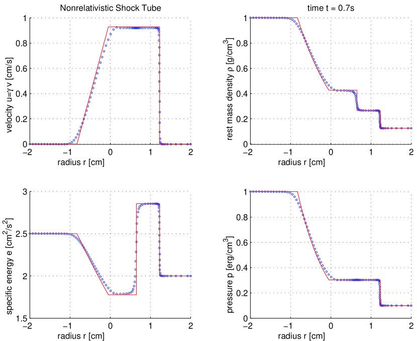
Figure 4: This figure shows a shocktube calculation with initial data leading to nonrelativistic velocities. The dots indicate the location of the grid points in the numerical solution. The solid line represents the analytical solution. In a time dependent visualization of this graph one would observe the grid points moving in accordance with the shock front. It is mainly the space coordinate of a grid point in the shock front that changes value, and not so much the represented physical state.

The comparison of the numerical and the analytical results is shown in Fig. (4). As expected from the conservative formulation, the shock speed exactly matches the analytical solution and the jump conditions are fulfilled. Somewhat smoother transitions in the numerical calculation around the contact discontinuity and the rarefaction wave are on the one hand due to the smoothened initial state and on the other hand to the diffusion according to equation (33) that is given by the advection scheme.

In order to test also the relativistic regime, we set up initial conditions for a relativistic shock. The initial state is $\left\{u,\rho,e,p\right\}_{L}=\left\{0,1,2.5\times 10^{22},10^{22}\right\}$ for $r<r_{0}$ and $\left\{u,\rho,e,p\right\}_{R}=\left\{0,0.125,2\times 10^{22},10^{21}\right\}$ for $r>r_{0}$. The velocity $u$ reaches about half of the velocity of light. This is much more than expected in any supernova calculation and enough to distinguish relativistic effects in the result. In the reproduction of the exact solution, we followed the approach of Centrella & Wilson (1984) and replaced their numerical integration of equation (C13) with an analytical solution. Analytical solutions to the special relativistic shocktube problem in an inertial coordinate frame were also derived by Marti & Müller (1994). Note, however, that the comoving coordinates used in our code do not limit to a global inertial frame in the special relativistic limit. While the areal radius, $r$, the enclosed rest mass, $a$, and the velocity, $u$, share their definition in both, the comoving Misner-Sharp coordinates and the inertial Schwarzschild coordinates, the definition of coordinate time is not the same in these coordinate choices. The correspondence is straightforward for the region at rest in the inertial frame and the region containing the matter between the contact discontinuity and the shock front because it is instantaneously accelerated to constant speed as the shock passes through. The fluid elements in the rarefaction wave have a more complicated velocity history and show an individual time lapse with respect to the inertial frame.

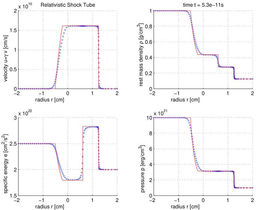
Figure 5: This figure shows a shocktube calculation that leads to relativistic velocities. The physical velocity $v=u/\gamma$ is large enough to distinguish relativistic effects. The dots indicate the location of the grid points in the numerical solution. The solid line represents the analytical solution. Note that the time measured in our comoving coordinates differs from the time measured in an inertial frame.

In Fig. (5) we compare the numerical solution to the analytical solution. This test demonstrates the accurate implementation of the special relativistic conservation laws that lead to the correct relativistic shock jump conditions.

4.3 Oppenheimer-Snyder dust collapse

The collapse of a uniform and pressureless dust cloud was first calculated in general relativity by Oppenheimer & Snyder (1939). Although most of the relativistic terms vanish for negligible pressure, this test problem is often recommended for general relativistic hydrocodes. It mainly tests the implementation of the momentum equation, because each fluid element behaves like a free particle in the self-gravitating pressureless gas. Initial configuration is a dust cloud of two solar masses with a density of $\rho=10^{8}gcm^{-3}$. In order to assure a negligible pressure, we set the initial temperature in the dust cloud to $T=10^{-5}MeV$. We had to switch off the adaptive grid for this run because spurious variations in the temperature profile lead to grid motions with advection inaccuracies that showed a positive feedback on the temperature variations.

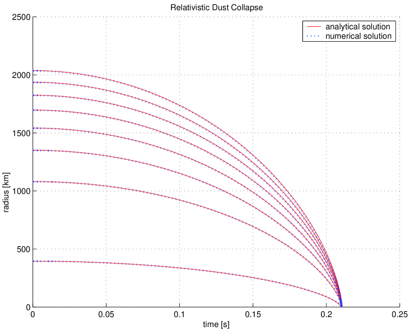
Figure 6: This figure shows the collapse of a homologous dust cloud in comoving coordinates. The numerical solution (dots) can hardly be distinguished from the analytical solution (solid lines) at early times. The lines represent mass traces at enclosed baryon masses of $[0.013,0.266,0.519,0.772,1.03,1.28,1.53,1.78]$ solar masses.

The result presented in Fig. (6) demonstrates that the match of the lapse function to the Schwarzschild metric outside of the cloud and that the discretization of the momentum equation are fine.

4.4 Homologous collapse

Here we present the homologous collapse that was first analyzed by Goldreich & Weber (1980). Again we use a polytropic equation of state with $p=\rho T/m_{b}$ and $e=(\gamma-1)^{-1}T/m_{b}$, where $T$ is the temperature and $\gamma=4/3$ the adiabatic index. With this equation of state, $p=(\gamma-1)\rho e$, one easily derives the time derivative

$$\frac{d}{dt}\left(\frac{p}{\rho^{\gamma}}\right)=\frac{\gamma-1}{\rho^{\gamma-1}}\left[\frac{de}{dt}+p\frac{d}{dt}\left(\frac{1}{\rho}\right)\right]=0.$$ (80)

Thus, the quantity $p/\rho^{\gamma}$ is expected to remain constant during the dynamical evolution. Our finite difference representation is chosen to conserve total energy to machine precision. The check for constant entropy in an adiabatic evolution therefore provides important information about the accuracy of the evolution of the internal energy. We run this test with the same artificial viscosity as in the realistic simultions in order to check its (non-)influence during the homologous compression in the collapse phase. Following Yamada (1997) we start with a hydrostatic isentropic state with central density $\rho_{c}=10^{8}$ g cm^-3 and temperature $T_{c}=0.2$ MeV. This configuration is uniformly cooled until we achieve marginal stability. We then reduce the pressure further by a total of $3$% (Goldreich & Weber, 1980), distributed over $300$ time steps. This leads to a smooth transition into collapse without initiating pressure waves that disturb the infall of the surface and lead to dissipation of kinetic energy in small shocks. We update the surface pressure proportionally to the evolution of the central pressure in order to prevent the surface from drifting out of the homologous motion owing to the lack of an outer part of the star. The test is carried out in the Newtonian limit, the fully relativistic run shows a less homologous velocity profile, but similar deviations in the enetropy.

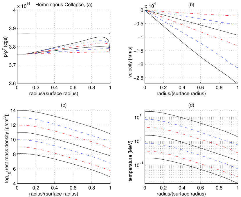
Figure 7: The homologous collapse of an isentropic polytrope is shown. Snapshots are taken when the central density reaches $[10^{8},10^{9},10^{10},10^{11},10^{12},10^{13},10^{14}]$ g cm^-3. Graph (a) shows the entropy evolution. The uppermost solid line belongs to the initial state. The lowermost dash-dotted line belongs to a central density of $10^{9}$ g cm^-3 and clearly shows the $3$% pressure reduction applied to initiate the collapse. The entropy deviation grows with increasing compactness. Graph (b) shows the velocity profiles. Graph (c) and (d) visualize the selfsimilar evolution of density and temperature.

The homologous collapse of an isentropic polytrope is shown in Fig. (7). Snapshots are taken for every decade in the central density. The radius of the profiles is normalized to the surface radius. Graph (a) shows the entropy evolution. The uppermost solid line belongs to the initial state. The lowermost dash-dotted line belongs to a central density of $10^{9}$ g cm^-3 and clearly monitors the $3$% pressure reduction applied to initiate the collapse. The entropy deviation grows with increasing compactness, but does not exceed the $3$% level until nuclear density is achieved in the center of the star. Graph (b) shows the nicely homologous velocity profiles with the velocity being proportional to the radius. Graph (c) and (d) visualize the selfsimilar evolution of density and temperature.

4.5 Comparison to PPM

Finally, we compare the shock tube result calculated with AGILE to the shock tube data provided by Raph Hix and Alan Calder from the EVH-1 implementation of PPM. Piecewise Parabolic Methods became a standard in hydrodynamics codes while conventional finite difference schemes gathered some patina, illustrated by their dependence on the unspeakable artificial viscosity.

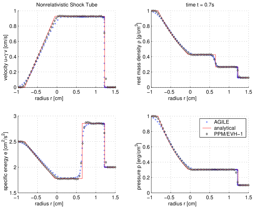
Figure 8: A nonrelativistic shocktube calculation comparing the results of AGILE and EVH-1. Both codes use $100$ grid points.

In Fig. (8), a comparison between the two methods is shown and related to the analytical solution. The solution of EVH-1 was calculated on $100$ equidistant grid points while AGILE used the same number of adaptive grid points. The reconstruction routines in EVH-1 do not implement a contact discontinuity steepening. A flattening parameter $f\leq 1$ is introduced to provide additional dissipation in the shock if a relative pressure jump exceeds $\varepsilon=0.33$ as defined by Colella & Woodward (1984) in Eq. (A.1). Following their prescription given in Eq. (A.2), this flattening parameter has been set to

$$\tilde{f}_{j}=1-\max\left(0,\left(\frac{p_{j+1}-p_{j-1}}{p_{j+2}-p_{j-2}}-\omega^{(1)}\right)\omega^{(2)}\right)$$ (81)

with $\omega^{(1)}=0.75$ and $\omega^{(2)}=5$. In AGILE, we have set a relatively small artificial viscosity with $\Delta l=2\times 10^{-3}$ cm in order to bring the misunderstanding about accuracy and artificial viscosity into prominence. The adaptive grid technique renders an unrivalled resolution in the shock front. A simulation on an equidistant grid would require $32000$ grid points to achieve a similar resolution at the shock. Moreover, the shock position and plateaus in the physical state are accurate. With a conservative formulation of the equations, the implicit algorithm solves numerically for the same jump conditions at the shock front as are solved analytically in a Riemann solver. The artificial viscosity only affects the shock width and provides the means for energy dissipation in the shock that is always present in a realistic fluid, even if the shock spreads over a narrower spatial range. The weakness of the adaptive grid, however, is the rarefaction wave. The diffusivity induced by advection on the dynamical adaptive grid as discussed in section 3.2 is responsible for the more indistinct rarefaction wave and contact discontinuity. According to equation (33), the artificial diffusion is large at increased grid spacing and high grid velocities. As expected, the PPM result shows less difficulty in the rarefaction wave, owing to its more uniform grid point distribution and smaller diffusivity. The run with EVH-1 required $40$ time steps with $4\times 10^{-4}$ CPU seconds per explicit time step on an IBM RS/6000 SP, the run with AGILE required $429$ time steps with $0.0713$ CPU seconds per implicit time step. $295$ time steps were used until physical time $0.35$ s and $134$ time steps were needed from $0.35$ to $0.7$ s. The efficiency increases in the second part of the simulation because, as illustrated in Fig. (2), the adaptive grid can take advantage of the self-similarity of the flow. About $30\%$ of the computational effort is spent with the inversion of the Jacobian. There are many ways to compare the performance depending on the importance of specific features. If one would request the same maximum resolution, the number of time steps required in EVH-1 would dramatically scale up by a factor of $320$ due to the Courant restriction on the time step. It is also important to note that the CPU time per time step is not relevant for the realistic applications we have in view. The computational effort is dominated by the radiation transport or the nuclear reaction network. Important is the overall number of zones and the ability to allocate them in regions with interesting physics. Moreover, the total computational effort will be proportional to the number of time steps. In the shock tube calculation, the Courant condition of explicit schemes is only challenged by resolution. In the supernova application, the restriction is much more severe in the compact proto-neutron star, where the sound speed quickly reaches a third of the velocity of light.

5 Conclusion

We report on AGILE, a first order implicit solver for stiff algebro-differential equations. AGILE builds the Jacobian by automatized numerical finite differences. It is therefore flexible with respect to changes and extensions in the physical equations and robust against programming errors in the now obsolete implementation of the Jacobian. As discussed in the introduction, implicit finite differencing is especially useful in astrophysical applications where the characteristic time scale of physical processes varies by orders of magnitude.

In spherical symmetry, we have written the Einstein equations in comoving coordinates and conservative form. These equations are implemented in a module for AGILE to obtain a spherically symmetric general relativistic hydrodynamics code. We recognize that a dynamical adaptive grid is nothing else than a specific choice of shift vectors in the view of a general relativistic 3+1 decomposition. The adaptive grid technique of Winkler, Norman, & Mihalas (1984) and Dorfi & Drury (1987), that was developed for Newtonian hydrodynamics, has been extended to relativistic space-time and used as a recipe for a stable implementation of shift vectors that focus the numerical work to physically important regions in the simulation.

With an application in stellar core collapse and supernova simulations in view, special care of energy conservation was taken. We present the detailed wrinkles in our finite difference representation of the physical equations. Our guidelines were (i) a consistent discretization of interdependent constituents to achieve an exact implementation of physical conservation laws, (ii) avoidance of cancellation errors by the independent evolution of small quantities, (iii) the absorption of numerical defects into the physical concept of viscosity for an overall consistency. Thus, the discretization of the total energy equation is matched to the finite difference representation of the momentum and internal energy equation and leads to energy conservation at machine precision. We quantify the diffusion introduced by advection in the finite difference representation of the momentum equation. Energy conservation requires a compensating pressure term in the energy equation that we consistently absorbe into the concept of artificial viscosity. Our artificial viscosity is based on the tensor viscosity approach of Tscharnuter & Winkler (1979) that was extended to general relativity by direct inclusion of the viscous stress-energy tensor into the derivation of the Einstein equations (Liebendörfer, Mezzacappa, & Thielemann, 2001).

We achieve accurate results in the standard test problems for the supernova application, i.e., Sedov point blast explosion, nonrelativistic shock tube, relativistic shock tube, Oppenheimer-Snyder dust collapse, and in the homologous collapse. We also compare our shock tube solution to a simulation with the Piecewise Parabolic Method and demonstrate a superior resolution of the shock with the adaptive grid. The overall reduction of computational zones, without compromise in the resolution of physically important regions, is especially helpful if the hydrodynamics code is coupled to computationally more expensive processes, as e.g. Boltzmann radiation transport or a nuclear reaction network. The comparison with PPM confirms that the artificial viscosity in the adaptive grid technique does not affect the accuracy of the shock speed and the fulfillment of the correct jump conditions. However, with the low order advection scheme chosen in this work, considerable diffusion happens in the rarefaction wave where the adaptive grid does not opt for a high resolution.

A previous version of AGILE has been used to simulate the hydrodynamical part in X-ray burst simulations on an accreting neutron star (Rembges, 1999). An AGILE module implementing general relativistic hydrodynamics in polar slicing and radial gauge has been tested and extended by Müller (2000) to study the effect of dark matter in the formation of supermassive black holes in the early universe. A Newtonian module in Lagrangian coordinates has been used in stellar core collapse and postbounce evolution simulations with complete O(v/c) Boltzmann neutrino transport (Mezzacappa et al., 2001). The module described in this paper, in combination with general relativistic Boltzmann neutrino transport, lead to the general relativistic simulation of stellar core collapse and postbounce evolution (Liebendörfer et al., 2001).

References

- Arnowitt, Deser, & Misner (1962) Arnowitt, A., Deser, S., & Misner, C. W. 1962, in Gravitation: An Introduction to Current Research, ed. L. Witten (New York: Wiley)
- Bader & Deuflhard (1983) Bader, G., & Deuflhard, P., Numer. Math., 41, 373
- Bruenn, DeNisco, & Mezzacappa (2001) Bruenn, S. W., DeNisco, K. R., & Mezzacappa, A. 2001, ApJ, 560, 326
- Centrella & Wilson (1984) Centrella, J., & Wilson, J. R. 1984, ApJS, 54, 229
- Colella & Woodward (1984) Colella, P., & Woodward, P., 1984, J. Comput. Phys., 54, 174
- Courant, Friedrichs, & Lewy (1928) Courant, R., Friedrichs, K. O., & Lewy H. 1928, Math. Ann., 100, 32
- Dorfi & Drury (1987) Dorfi, E. A., & Drury, L. O’C. 1987, J. Comput. Phys., 69, 175
- Dorfi & Gautschi (1989) Dorfi, E. A., & Gautschi, A. 1989, in The Numerical Modelling of Nonlinear Stellar Pulsations, ed. J. R. Buchler (Dordrecht: Kluwer Academic Publishers)
- Eggleton (1971) Eggleton, P. P. 1971, MNRAS, 151, 351
- Gehmeyr & Mihalas (1994) Gehmeyr, M., & Mihalas, D. 1994, Physica D, 77, 320
- Goldreich & Weber (1980) Goldreich, P., & Weber, S. V. 1980, ApJ, 238, 991
- Harten & Hyman (1983) Harten, A., & Hyman, J. M. 1983, J. Comp. Phys. 50,235
- Henyey et al. (1959) Henyey, L. G., Wilets, L., Bohm, K. H., Lelevier, R., & Levee, R. D. 1959, ApJ, 129, 628
- Landau & Lifschitz (1991) Landau, L. D., & Lifschitz, J. M. 1991, Lehrbuch der Theoretischen Physik, Vol. 6 (5th ed.; Frankfurt: Harri Deutsch)
- Liebendörfer & Rosswog (1998) Liebendörfer, M., & Rosswog, S. K. 1998, Proc. of the 9th Workshop on Nuclear Astrophysics, ed. W. Hillebrandt & E. Müller (Garching b. München: MPA), 111
- Liebendörfer & Thielemann (2000) Liebendörfer, M., & Thielemann, F. K. 2000, in Nineteenth Texas Symposium on Relativistic Astrophysics, ed. E. Aubourg, T. Montmerle, J. Paul, & P. Peter (Amsterdam: Elsevier Science B. V.), CD-ROM 07/13
- Liebendörfer (2000) Liebendörfer, M. 2000, Consistent Modeling of Core-Collapse Supernovae in Spherically Relativistic Space-Time, Ph.D. thesis (Basel: University of Basel)
- Liebendörfer, Mezzacappa, & Thielemann (2001) Liebendörfer, M., Mezzacappa, A., & Thielemann, F.-K. 2001, Phys. Rev. D, 63, 104003
- Liebendörfer et al. (2001) Liebendörfer, M., Mezzacappa, A., Thielemann, F.-K., Messer, O. E. B., Hix, W. R., & Bruenn, S. W. 2001, Phys. Rev. D, 63, 103004
- Mair (1990) Mair, G. 1990, Die frühe Lichtkurve der Supernova 1987A, Ph.D. thesis (München: Technische Universität München)
- Marti & Müller (1994) Marti, J. M., & Müller, E. 1994, J. Fluid. Mech., 258, 317
- May & White (1967) May, M. M., & White, R. H. 1967, J. Comput. Phys., 7, 219
- Mezzacappa et al. (2001) Mezzacappa, A., Liebendörfer, M., Messer, O. E. B., Hix, W. R., Thielemann, F.-K., & Bruenn, S. W. 2001, Phys. Rev. Lett., 86, 1935
- Misner & Sharp (1964) Misner, C. W., & Sharp, D. H. 1964, Phys. Rev. B, 136, 571
- Müller (2000) Müller, H. 2000, Bildung supermassiver schwarzer Löcher im frühen Universum, Diploma thesis (Heidelberg: Landessternwarte Heidelberg-Königstuhl)
- Noh (1978) Noh, W. F. 1978, J. Comput. Phys., 72, 78
- Norman & Winkler (1986) Norman, M. L., & Winkler, K.-H. 1986, in Astrophysical Radiation Hydrodynamics, ed. K.-H. Winkler & M. L. Norman, Vol. 188 (NATO Advanced Study Institute, Series C; New York: Plenum), 449
- Oppenheimer & Snyder (1939) Oppenheimer, J. R., & Snyder, H. 1939, Phys. Rev., 56, 455
- Rampp & Janka (2000) Rampp, M., & Janka, H. T. 2000, ApJ, 539, L33
- Rembges (1999) Rembges, F. 1999, Hot Hydrogen Burning in Accreting Neutron Stars, Ph.D. thesis (Basel: University of Basel)
- Romero et al. (1996) Romero, J. V., Ibanez, J. M., Marti, J. M., & Miralles, J. A. 1996, ApJ, 462, 839
- Schinder & Bludman (1989) Schinder, P. J., & Bludman, S. A. 1989, ApJ, 346, 350
- Sedov (1959) Sedov, L. I. 1959, Similarity and Dimensional Problems in Mechanics (New York: Academic)
- Smarr & York (1978) Smarr, L. & York, J. W. 1978, Phys. Rev. D, 17, 2529
- Sod (1978) Sod, G. A. 1978, J. Comput. Phys., 27, 1
- Swesty (1995) Swesty, F. D. 1995, ApJ, 445, 811
- Taylor (1950) Taylor, G. 1950, Proc. R. Soc. Lond. A, 201, 159
- Tscharnuter & Winkler (1979) Tscharnuter, W. M., & Winkler, K. H. 1979, Comput. Phys. Comm., 18, 171
- Von Neumann & Richtmyer (1950) Von Neumann, J., & Richtmyer, R. D. 1950, J. Appl. Phys., 21, 232
- Winkler, Norman, & Mihalas (1984) Winkler, K.-H., Norman, M. L., & Mihalas, D. 1984, J. Quant. Spectrosc. Radiat. Transf., 31, 473
- Winkler & Norman (1986) Winkler, K.-H., & Norman, M. L. 1986, in Astrophysical Radiation Hydrodynamics, ed. K.-H. Winkler & M. L. Norman, Vol. 188 (NATO Advanced Study Institute, Series C; New York: Plenum), 73
- Yamada (1997) Yamada, S. 1997, ApJ, 475, 720