The Distribution of Pressures in a Supernova-Driven Interstellar Medium

Abstract

Observations have suggested substantial departures from pressure equilibrium in the interstellar medium (ISM) in the plane of the Galaxy, even on scales under 50 pc. Nevertheless, multi-phase models of the ISM assume at least locally isobaric gas. The pressure then determines the density reached by gas cooling to stable thermal equilibrium. We use two different sets of numerical models of the ISM to examine the consequences of supernova driving for interstellar pressures. The first set of models is hydrodynamical, and uses adaptive mesh refinement to allow computation of a $1\times 1\times 20$ kpc section of a stratified galactic disk. The second set of models is magnetohydrodynamical, using an independent code framework, and examines a (200 pc)³ periodic domain threaded by magnetic fields. Both of these models show broad pressure distributions with roughly log-normal functional forms produced by both shocks and rarefaction waves, rather than the power-law distributions predicted by previous work, with rather sharp thermal pressure gradients. The width of the distribution of the logs of pressure in gas with $\log T<3.9$ is proportional to the rms Mach number in that gas, while the distribution in hotter gas is broader, but not so broad as would be predicted by the Mach numbers in that gas. Individual parcels of gas reach widely varying points on the thermal equilibrium curve: no unique set of phases is found, but rather a dynamically-determined continuum of densities and temperatures. Furthermore, a substantial fraction of the gas remains entirely out of thermal equilibrium. Our results appear consistent with observations of interstellar pressures, and suggest that the pressures observed in molecular clouds may be due to ram pressure rather than gravitational confinement.

1 Introduction

Theoretical models of the interstellar medium (ISM) have generally followed Spitzer (1956) in assuming that the interstellar gas is in pressure equilibrium. Field, Goldsmith & Habing (1969; hereafter FGH) demonstrated that the form of the interstellar cooling and heating curves for temperatures below about $10^{4}$ K allowed a range of pressures in which two isobaric phases could exist in stable thermal equilibrium. Although the details of this model turned out to be incorrect, due to their assumption of a cosmic ray flux much higher than subsequently observed, Wolfire et al. (1995) demonstrated that photoelectric heating of polycyclic aromatic hydrocarbons or other very small dust grains could recover a two-phase model for the neutral ISM. McKee & Ostriker (1977; hereafter MO) used a similar framework for the cold ISM, but incorporated the suggestion by Cox & Smith (1974) that supernovae (SNe) would create large regions of hot gas with $T\sim 10^{6}$ K, to produce a model of a three-phase medium. They were the first to relax the assumption of global pressure equilibrium, noting that SN remnants (SNRs) would have varying pressures. They assumed only local pressure equilibrium at the surfaces of clouds in order to determine conditions there.

Measurements of the ISM pressure were performed using Copernicus observations of ultraviolet (UV) absorption lines from excited states of C i by Jenkins & Shaya (1979) and Jenkins, Jura & Loewenstein (1983). They found greater than an order of magnitude variation in pressures in the cold gas traced by the C i, with most of the gas having pressures $P/k<10^{4}$ K cm^-3, but a small fraction reaching pressures $P/k>10^{5}$ K cm^-3. These findings have recently been confirmed and extended using Space Telescope Imaging Spectrograph (STIS) observations by Jenkins & Tripp (2001). Bowyer et al. (1995) compared the pressure derived from the observation with the Extreme UV Explorer of a shadow cast by a cloud of neutral hydrogen, with the pressure of the warm cloud surrounding the Sun. They found the local pressure of 730 K cm^-3 to be a factor of 25 lower than the average pressure measured along the 40 pc line of sight to the interstellar cloud of $1.9\times 10^{4}$ K cm^-3. McKee (1996) argued that these estimates were too extreme, but nevertheless concluded that the observations showed a pressure variation of at least a factor of five.

In this paper we show that dynamical models of a SN-driven interstellar medium do not produce an isobaric medium controlled by thermal instability, but rather a medium with a broad pressure distribution controlled by the dynamics of turbulence, with rarefaction waves being as important as shocks in setting local pressures. Although the cooling curve may determine local behavior, the pressure of each parcel is set dynamically by flows primarily driven by distant SNe. The theory of polytropic, compressible turbulence described by Passot & Vázquez-Semadeni (1998; hereafter PV98) seems able to explain some of our results, with careful application.

Gazol et al. (2001) demonstrate that turbulence driven by ionization heating results in nearly half of the gas lying in thermally unstable regions, in agreement with the observations of Heiles (2001). Earlier dynamical models of the ISM have been reviewed by Mac Low (2000). Models including SN driving were first done in two dimensions by Rosen & Bregman (1995), and have since been done by a number of other groups. Vázquez-Semadeni, Passot & Pouquet briefly discussed the pressure structure in a two-dimensional hydrodynamical model including only photoionization heating. In three dimensions, Avillez (2000) used an adaptive mesh refinement code to compute the evolution of a $1\times 1\times 20$ kpc vertical section of a galactic disk, while Korpi et al. (1999) used a single grid magnetohydrodynamical (MHD) code to model an SN-driven galactic dynamo. They briefly discuss the pressure structure as well. All of these computations show that the interactions between SNRs drive turbulent flows throughout the ISM, and that radiative cooling of compressed regions produces cold, dense clouds with relatively short lifetimes.

We here study in substantially more detail than previous workers the pressure distribution in both hydrodynamical and MHD models of the SN-driven ISM. For the hydrodynamical case, we use the same code as Avillez (2000), including stratification, radiative cooling, and both clustered and isolated SNe. For the MHD case, we use the Riemann framework of Balsara (2000) in single-grid mode on a 200 pc cube with periodic boundary conditions on all sides, including both radiative cooling and heating, as well as isolated SNe. Although these two models are not directly comparable, they do allow us to examine a wide range of physical conditions and draw some firm conclusions about the behavior of the interstellar pressures.

In § 2 we describe the different models we use in more detail. We then give two different analytic approaches to the question of the pressure distribution in the SN-driven ISM in § 3, derived from the work of MO and PV98. In § 4 we use the numerical results to demonstrate that the SN-driven ISM is far from isobaric, with order of magnitude pressure variations, but that the distribution of pressures takes on a log-Gaussian form that can be very well described. These results are compared to observations in § 5, and the paper is summarized in § 6.

2 Models

2.1 Stratified Gas Dynamical

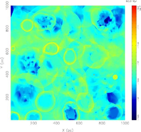
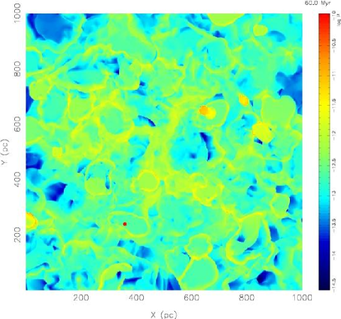
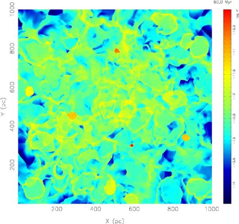
Figure 2: Two-dimensional slices through three-dimensional stratified models in the Galactic plane at a time of 60 Myr (20 Myr earlier than in Figure 1) showing pressure for SN rates of (a) the galactic rate (model S2), (b) six times that rate ( model S3), and (c) ten times that rate (model S4). Color bars indicate the scale of pressure.

The first type of model we use is a three-dimensional computation of the disk-halo interaction in an SN-driven ISM using an adaptive-mesh-refinement (AMR) hydrodynamics code on a $1\times 1\times 20$ kpc region of the Galactic disk, described by Avillez (2000). The model includes a fixed gravitational field provided by the stars in the disk, and radiative cooling assuming optically thin gas in collisional ionization equilibrium. The radiative cooling function is a tabulated version of that shown in Figure 2 of Dalgarno & McCray (1972) with an ionization fraction of 0.1 at temperatures below $10^{4}$ K and a temperature cutoff at 100 K. (No pervasive heating term is included in this model, however, and so it never reaches thermal equilibrium.) The interstellar gas is initially distributed in a smooth disk with the vertical distribution of the cool and warm neutral gas given by Lockman, Hobbs, & Shull (1986) and summarized in the Dickey & Lockman (1990) distribution. In addition, an exponential profile representing the $z-$distribution of the warm ionized gas with a scale-height of 1 kpc in the Galaxy as described in Reynolds (1987) is used.

SNe of types Ib, Ic, and II are explicitly set up at random locations isolated in the field ($40\%$) as well as in locations where previous SNe occurred, representing OB associations ($60\%$). The latter are set in a layer of a mean half thickness of 46 pc (from the midplane) following the distribution of the molecular gas in the Galaxy, while the isolated SNe are set in a layer having half thickness of 100 pc. The first SNe in associations occur in locations where the local density is greater than 1 cm^-3. No density threshold is used to determine the location where isolated SNe should occur, because their progenitors drift away from the parental association and therefore, their site of explosion is not correlated with the local density. The SNe are set up at the beginning of their Sedov phases, with radii determined by their progenitor masses. Type II SNe come from early B stars with masses $7.7M_{\odot}\leq M\leq 15M_{\odot}$ while type Ib and Ic SNe have progenitors with masses $M\geq 15M_{\odot}$ (Tammann, Löffler, & Schröder 1994). In our model the maximum mass allowed for an O star is 30 $M_{\odot}$. Avillez (2000) describes in detail the algorithm used to set up the isolated and clustered SNe during the simulations.

These simulations use the piecewise-parabolic method of Colella & Woodward (1984), a third-order scheme implemented in a dimensionally-split (Strange 1968) manner that relies on solutions of the Riemann problem in each zone rather than on artificial viscosity to follow shocks. During the simulation, the mesh is refined periodically in regions with sharp pressure variations using the AMR scheme. The local increase of the number of cells corresponds to an increase in resolution by a factor of two (that is, every refined cell is divided into eight new cells). At every new grid the procedure outlined above is carried out, followed by the correction of fluxes between the refined and coarse grid cells. The adaptive mesh refinement scheme is based on Berger & Colella (1989), but the grid generation procedure follows that described in Bell et al. (1994).

The computational domain has an area of 1 kpc² and a vertical extension of 10 kpc on either side of the midplane. In the simulations discussed here, AMR is used in the layer $\left|z\right|\leq 500$ pc. In the highest resolution runs, three levels of refinement are used, yielding a finest resolution of 1.25 pc. For $\left|z\right|>500$ pc the resolution is 10 pc. Periodic boundary conditions are used at the vertical boundaries, while outflow boundary conditions are used at the top and bottom boundaries. The loss of matter through the upper and lower boundaries after 1 Gyr of simulation amounts to $12\%$ of the total initial mass used at the beginning of the simulations (Avillez 2000).

The rates of occurrence of SNe types Ib, Ic in the Galaxy are $2\times 10^{-3}$ yr^-1, while those of type II occur at $1.2\times 10^{-2}$ yr^-1 (Cappellaro et al. 1997). The total rate of these SNe in the Galaxy is $\tau_{\rm gal}=1.4\times 10^{-2}$ yr^-1, corresponding to a rate of one SN every 71 yr. These rates are normalized to the volumes of the stellar disk used in the simulations. In the current work we report simulations, as described in Table 1, using three SN rates: $\tau/\tau_{\rm gal}=1$, 6, and 10. For each rate of SNe we run two simulations with different finest resolutions of the AMR hierarchy: 1.25 and 2.5 pc. In the cases reported here, we ran the simulations for 200 Myr, long enough to establish the disk-halo circulation and reach a steady state in the simulated thick gas disk.

2.2 Magnetohydrodynamical

The MHD calculations were done using the RIEMANN framework for computational astrophysics, which is based on higher-order Godunov schemes for MHD (Roe and Balsara 1996; Balsara 1998a,b), and incorporates schemes for pressure positivity (Balsara & Spicer 1999a), and divergence-free magnetic fields, (Balsara & Spicer 1999b). (The framework also includes parallelized adaptive mesh refinement [Balsara and Norton 2001; Balsara 2001], though that capability is not used in the present paper).

In the models presented here, we solve the ideal MHD equations including both radiative cooling and pervasive heating in a (200 pc)³ periodic computational box, mostly using a grid of 128³ cells. We start the simulations with a uniform density of $2.3\times 10^{-24}$ g cm^-3, threaded by a uniform magnetic field in the $x$-direction with strength 5.8 $\mu$G, a factor of roughly two stronger than that observed in the Milky Way disk. This very strong field maximizes the effects of magnetization on the turbulence, and may be seen as the other extreme from our hydrodynamical models. Behavior common to both sets of models can be deduced to be fairly independent of the magnetic field.

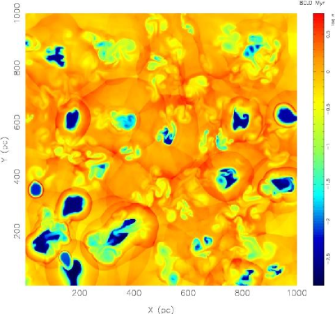
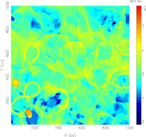
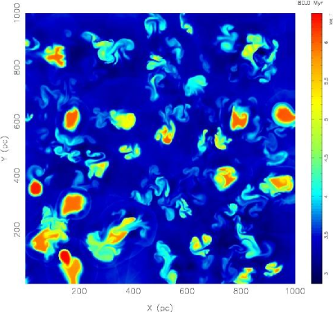
Figure 1: Two-dimensional slices through the three-dimensional stratified model S2 in the Galactic plane at a time of 80 Myr showing (a) density, (b) thermal pressure, and (c) temperature. Color bars indicate the scale of each quantity.

For the cooling, we use a tabulated version of the radiative cooling curve shown in Figure 1 of MacDonald and Bailey (1981), which is based on the work of Raymond, Cox & Smith (1976) and Shapiro and Moore (1976). (It falls smoothly from temperatures of order $10^{5}$ K to $10^{2}$ K, not incorporating a sharp cutoff at $10^{4}$ K due to the turnoff of Ly$\alpha$ cooling.) In order to prevent the gas from cooling below zero, we set the lower temperature cutoff for the cooling at 100 K. We also include a diffuse heating term to represent processes such as photoelectric heating by starlight, which we set constant in both space and time. We set the heating level such that the initial equilibrium temperature determined by heating and cooling balance is 3000 K. Since the cooling time is usually shorter than the dynamical time, we adopt implicit time integration for the cooling and heating terms.

We explode SNe at a rate of one every 0.1 Myr in our box, twelve times higher than our present Galactic rate, corresponding to a mild starburst like M82. The SNe are permitted to explode at random positions. To avoid extremely high initial expansion velocities, we do not allow SNe to explode in regions with density less than 0.1 cm^-3; however, unlike Korpi et al. (1999), this does still allow SNe to explode within the shells of pre-existing remnants. They are not focussed into associations, however, unlike in the stratified models.

Each SN explosion dumps 10⁵¹ erg thermal energy into a sphere with radius 5 pc. The evolution of the system is determined by the energy input from SN explosions and diffuse heating and the energy lost by radiative cooling. We follow the simulations to the point where the total energy of the system, as well as the energy in the thermal, kinetic and magnetic variables, has reached a quasi-stationary value for several million years.

3 Analytic Theories

3.1 Non-interacting Supernova Remnants

The two-phase theory of FGH assumed pressure equilibrium throughout the ISM, with densities and temperatures fully regulated by heating and cooling processes acting on timescales shorter than the dynamical timescale of the gas. The introduction of SN explosions by Cox & Smith (1974) and MO required relaxation of the assumption of pressure equilibrium, at least inside of expanding SNRs. In particular, Jenkins et al. (1983) emphasized that MO implicitly makes a prediction of the spectrum of pressure fluctuations expected from the passage of SNRs expanding in a clumpy medium.

The theory of pressure fluctuations begins from the scaling in MO, Appendix B, of the pressure of the low-density intercloud medium $P$ as a function of the probability $Q(R)$ of a point being within a SNR with radius at least $R$,

$$P=P_{c}\left\{\begin{array}[]{ll}(Q/Q_{c})^{-9/14}&\mbox{ for $Q\leq Q_{c}$}\\ 0.5(Q/Q_{c})^{-0.9}&\mbox{ for $Q>Q_{c}$},\end{array}\right.$$ (1)

where $Q_{c}$ is the probability of a point being within a SN remnant large enough for the swept-up shell of intercloud medium to have cooled, and $P_{c}$ is the corresponding pressure of such a remnant. For typical values in the Milky Way, including a SN rate $S=10^{-13}$ pc^-3 yr^-1, MO find by balancing a number of observational considerations that likely values for these parameters are $Q_{c}=1/2$, and $P_{c}/k=10^{3.67}$ cm^-3 K (see their eq. 9). Equation 1 can then be inverted to give the probability $Q(P)$ of a point being within a SN remnant with pressure at least $P$, as written in Jenkins et al. (1983).

The probability $Q(P)$ represents a cumulative distribution. The corresponding differential probability distribution function (PDF) is given by $-dQ(P)$. In practice, we compute PDFs by constructing a histogram of pressure values, with bins of finite size $\Delta P$, so the PDF predicted by MO is

$$-(\partial Q/\partial P)\Delta P=\left\{\begin{array}[]{ll}\frac{14Q_{c}}{9P_{c}}\left(\frac{P}{P_{c}}\right)^{-23/9}\Delta P&\mbox{for $P>P_{c}$},\\ \frac{20Q_{c}}{9P_{c}}\left(\frac{P}{P_{c}}\right)^{-19/9}\Delta P&\mbox{for $P\leq P_{c}$}.\end{array}\right.$$ (2)

This PDF would diverge towards low pressures if it were not limited by the consideration that the pressure in an isolated SN remnant will not fall below the ambient pressure $P_{0}$, so that there must be a lower cutoff at that value. (MO give $P_{0}/k=10^{3.10}$ cm^-3 K for the same parameters given above.) This model predicts no pressures below the ambient value $P_{0}$.

3.2 Turbulence

An alternative approach to predicting the distribution of interstellar pressure fluctuations can be derived from recent work on properties of highly compressible turbulence by PV98, inspired by computations of isothermal turbulence by Padoan, Nordlund, & Jones (1997) and Vázquez-Semadeni (1994). PV98 considered the PDF of density in a turbulent, polytropic gas with pressure $P=K\rho^{\gamma}$, where $\gamma$ is the polytropic index. By making the assumption that the density fluctuations are built up by successive passages of shocks and rarefaction waves (Vázquez-Semadeni 1994) that act as a random multiplicative process, they were able to show that the density distribution ${\cal P}$ is a log-normal when the gas is isothermal ($\gamma=1$)

$${\cal P}(s)ds=\frac{1}{\sigma_{s}\sqrt{2\pi}}\exp\left[-\frac{(s-s_{0})^{2}}{2\sigma_{s}^{2}}\right]ds,$$ (3)

where the variable $s=\ln\rho/\rho_{0}$, and $\rho_{0}$ is the mean density of the region. The variance of the logs of the densities was found numerically to be

$$\sigma_{s}=M_{\rm rms},$$ (4)

where the scaled root mean square (rms) Mach number $M_{\rm rms}=v_{\rm rms}/c(\rho_{0})$, the ratio of the rms velocity to the sound speed at a density $\rho_{0}$, derivable from the polytropic law. By mass conservation, the shift of the peak given by $s_{0}=-0.5\sigma_{s}^{2}$. In the non-isothermal case ($\gamma\neq 1$), a density-dependent rescaling allows PV98 to derive a tilted log-normal form

$${\cal P}(s;\gamma)ds=C(\gamma)\exp\left[-\frac{s^{2}}{2M_{\rm rms}^{2}}-\alpha(\gamma)s\right]ds,$$ (5)

where $C(\gamma)$ is a normalization constant such that the integral over the distribution is unity, and $\alpha$ satisfies the relation $\alpha(2-\gamma)=1-\alpha(\gamma)$, but is independent of the strength of the turbulence.

From this formalism, we can derive the PDF in pressure ${\cal P}(P)$ by simply using the polytropic law. For convenience, we define $x=\log_{10}P$, so that

$$s=(x-x_{0})/(\gamma\epsilon),$$ (6)

where $x_{0}=\log_{10}P(\rho_{0})$ and $\epsilon=\log_{10}e$. Then the isothermal distribution becomes

$${\cal P}(x)dx=(\gamma\epsilon\sigma_{s}\sqrt{2\pi})^{-1}\exp\left\{-\frac{[(x-(x_{0}+\gamma\epsilon s_{0})]^{2}}{2(\gamma\epsilon)^{2}\sigma_{s}^{2}}\right\}dx,$$ (7)

and the nonisothermal distribution can be derived from equation (20) of PV98 to have the somewhat ungainly form

$${\cal P}(x;\gamma)dx=\frac{C(\gamma)}{\gamma\epsilon}\exp\left[-\frac{(x-x_{0})^{2}}{2(\gamma\epsilon)^{2}(v_{\rm rms}/c_{0})^{2}}\exp\left\{\frac{\gamma-1}{\gamma\epsilon}(x-x_{0})\right\}-\frac{\alpha(\gamma)(x-x_{0})}{\gamma\epsilon}\right]dx.$$ (8)

The dispersion of the decimal logs of the pressures is thus predicted in either case to be

$$\sigma_{x}^{2}=\gamma^{2}\epsilon^{2}(v_{\rm rms}/c_{0})^{2}.$$ (9)

In equation (8) the exponential factor multiplying the Gaussian $x^{2}$ term cuts it off on one side of the peak, allowing the dominance of the power-law term with slope given by $\alpha(\gamma)/\gamma\epsilon$, which was numerically found by PV98 to have the value 0.43 for $\gamma=1.5$. Below we will compare our numerical results to this formalism.

4 Numerical Results

4.1 Morphology

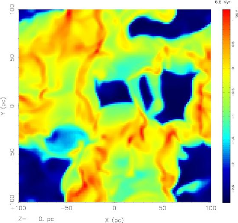
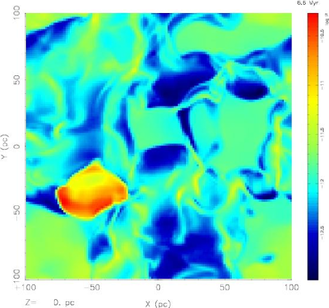
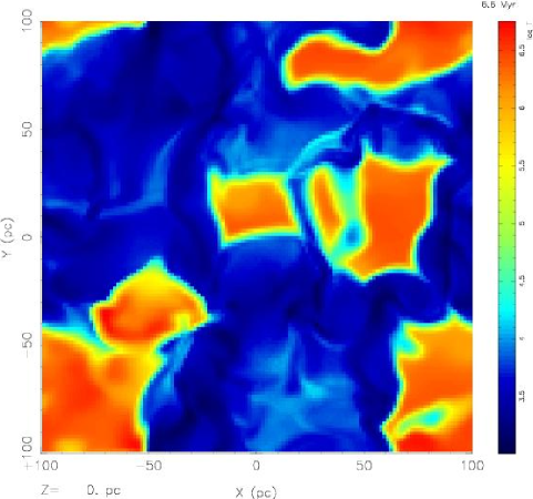
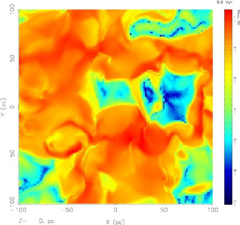
Figure 3: Two-dimensional slices through the three-dimensional MHD model M2, parallel to the magnetic field at a time of 6.6 Myr, showing density (upper left), thermal pressure (upper right), temperature (lower left), and magnetic pressure (lower right). Color bars indicate the scale of each quantity.

We now examine the pressure distribution in our numerical simulations of a SN-driven interstellar medium. In Figure 1 we show density, pressure, and temperature on cuts in the plane of the galaxy from stratified model S2 after it has reached equilibrium, in Figure 2 we compare pressure distributions from models S2, S3, and S4, with increasing SN rate, and in Figure 3 we show density, pressure, and temperature, as well as magnetic pressure, on cuts through the MHD model M2 parallel to the magnetic field. (The perpendicular direction appears identical, because the flows are strongly super-Alfvénic, with rms Alfvén number exceeding four.) Examination of the pressure images immediately shows a broad variation in pressures among different regions in all the models, including in regions not closely associated with young SNRs. Regions with pressures markedly lower than ambient are apparent.

Low-pressure regions tend to be associated with intermediate density regions in the hydrodynamical models, while in the magnetized models the very lowest thermal pressures are actually associated with substantial magnetic pressures, although there are also low-pressure regions similar to those in the hydrodynamical models. We will examine this more quantitatively further below. High temperature regions lie inside young SNRs, while low temperature regions have no uniform density and temperature correlation. The highest density regions have sizes of dozens of parsecs, and average densities approaching 100 cm^-3, typical of giant molecular clouds. This is consistent with the suggestion by Ballesteros-Paredes et al. (1999a) and Ballesteros-Paredes, Vázquez-Semadeni & Scalo (1999) that molecular clouds are formed and destroyed by the action of the interstellar turbulence. Isobaric thermal instabilities, as discussed by Hennebelle & Pérault (1999, 2000), Burkert & Lin (2000), Vázquez-Semadeni, Gazol, & Scalo (2000), and Gazol et al. (2001), must still be examined, however, by incorporation of appropriate cooling and heating models at low temperatures.

Even at SN rates ten or twelve times those characteristic of the Milky Way, the hot medium in our models does not have the pervasive, space-filling nature suggested by a simple interpretation of MO. Rather, discrete regions of hot gas are formed, occasionally intersect, and then seem to be dynamically mixed back into the warm gas that fills a substantial fraction of the space. This large-scale turbulent mixing, which can most clearly be seen in older remnants in Figure 1c, appears to substantially enhance the cooling rate, while sheets and filaments confined by nearby SNRs seem more effective at slowing down the expansion of SNRs than the isolated spherical clouds considered in MO. However, these results will need to be confirmed by more careful modeling in the future to ensure that numerical diffusion is not the main factor in reducing the amount of hot gas. The filling factors in the stratified model are discussed in more detail in Avillez (2000), where it is shown that the filling factor of the hot gas grows substantially above the disk plane, ultimately resulting in a galactic fountain above about 1 kpc, even at SN rates typical of the Milky Way.

4.2 Thermodynamic Relations

The first theories of the multi-phase ISM, such as FGH, postulated an isobaric medium. Since then, multi-phase models have commonly been interpreted as being isobaric, although MO and Wolfire et al. (1995) actually assume only local pressure equilibrium, not global, and MO considered the distribution of pressures, as described above in § 3.1. In multi-phase models, the heating and cooling rates of the gas have different dependences on the temperature and density, so that the balance between heating and cooling determines allowed temperatures and densities for any particular pressure. This balance can be shown graphically in a phase diagram, showing, for example, the allowed densities for any pressure (FGH; for a modern example, see Fig. 3(a) of Wolfire et al. 1995).

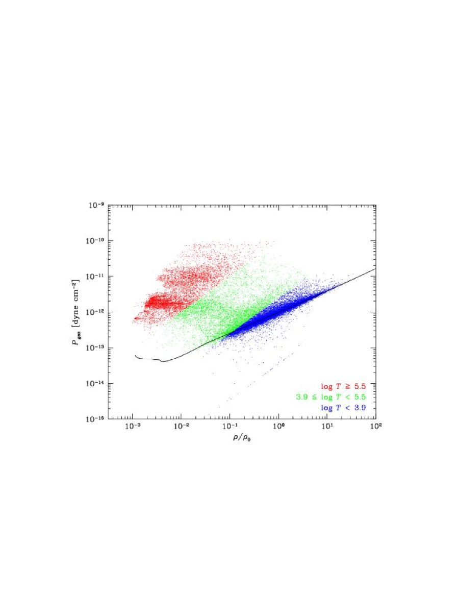
Figure 5: Scatter plot of pressure vs. density at $t=6.6$ Myrs in the MHD simulation M2, showing $32^{3}$ points sampled at intervals of four points in each direction. Note that for each density a wide variation in pressure is seen. Cool gas with $\log T<3.9$ is shown in blue, warm gas with $3.9<\log T<5.5$ in green, and hot gas with $\log T>5.5$ in red. The thermal equilibrium curve for the cooling and heating functions in this simulation is overlaid as a black line. (The line of points at the very bottom right corresponds to an absolute cutoff in the cooling at 100 K that was enforced on the temperature in this model.) Note that our cooling curve may artificially prevent much low-temperature gas from forming in this model.

In Figure 5, the thermal-equilibrium curve for the heating and cooling mechanisms included in the MHD models is shown as a black line. (The stratified models did not include any pervasive heating term and so have no region of true thermal equilibrium.) Only a single phase is predicted at high densities as our cooling curve did not include the physically-expected unstable region at temperatures of order $10^{3}$ K (Wolfire et al. 1995). Thus, if our model produced an isobaric medium, it would be expected to have a single low-temperature phase in uniform density given by the point at which the thermal-equilibrium curve crosses that pressure level. (Effectively, we would have the hotter two of the three phases proposed by MO.)

The scattered points in Figure 5 show the actual density and pressure of individual zones in the model. Many zones at low temperature do lie on the thermal equilibrium curve, but scattered all up and down it at many different pressures and densities, with no well-defined phase structure. Furthermore, a substantial fraction of the gas has not had time to reach thermal equilibrium at all after dynamical compression. It appears that pressures are determined dynamically, and the gas then tries to adjust its density and temperature to reach thermal equilibrium at that pressure. Most gas will land on the thermal equilibrium curve when dynamical times are long compared to heating and cooling times. This will still lead to all points within the range of pressures available along the thermal equilibrium line being occupied, rather than the appearance of discrete phases. Unstable regions along the thermal equilibrium curve (Gazol et al. 2001) and off it will also be populated, as observed by Heiles (2001), but not as densely, as gas will indeed attempt to heat or cool to a stable thermal equilibrium at its current pressure.

The range of pressures observed in our simulations is, in fact, broader than the region shown by Wolfire et al. (1995) to be subject to thermal instability. Even models that included a proper cooling curve would produce some gas at pressures incapable of supporting a classical multi-phase structure. The mixture of different pressures would, however, produce gas at both high and low densities, as well as a smaller fraction of gas at intermediate densities that has not yet reached thermal equilibrium. We will discuss the resulting density and temperature PDFs in upcoming work.

Under what conditions will the dynamical times indeed be long compared to heating and cooling times? We can attempt to calculate this for one of our MHD models by making rough analytical estimates of each. The dynamical time is

$$t_{\rm dyn}=L/v_{\rm rms},$$ (10)

where $L$ is a characteristic length scale, while the cooling time

$$t_{\rm cool}=E/\dot{E}=kT/n\Lambda,$$ (11)

where $E$ is the thermal energy, and $\dot{E}=n^{2}\Lambda(T)$ is the cooling rate as a function of temperature $T$. In model M2, the rms velocity $v_{\rm rms}=55\mbox{ km s}^{-1}$. If we take typical dynamical length scales of $L\sim 10$ pc, then $t_{\rm dyn}\simeq 0.2$ Myr. We tabulate $t_{\rm cool}$ from our cooling curve in Table 2, normalized to a density of $n=1$ cm^-3. (We note that model cooling times in gas at temperatures of $10^{3}\mbox{ K}\lesssim T\lesssim 10^{4}$ K are substantially less than physical values, as the MacDonald & Bailey cooling curve does not drop abruptly at $10^{4}$ K when Ly$\alpha$ cooling shuts off. However, the consequence of this is merely that our model overestimates the amount of gas that has reached thermal equilibrium: the scatter plot shown in Figure 5 should be even more uniformly filled.) At all temperatures $10^{3}$ K$<T<10^{7}$ K, we find that $t_{\rm cool}\ll t_{\rm dyn}$, especially at densities $n>1$ cm^-3, substantiating our description of the gas dynamics being more important than local thermodynamics in determining the thermodynamic properties.

The separation between dynamical and thermal timescales also sheds light on the study by Vázquez-Semadeni et al. (2000) on the effects of turbulence on thermal instability. That study suggested that turbulence erases the effects of thermal instability on the interstellar medium. What is suggested by our models is that turbulence probably didn’t erase the thermal instability entirely, but that the instability only acted locally, under the conditions set for it by the larger-scale turbulent flow. Also, thermal instability becomes less important in determining the overall distribution of pressures and temperatures when much of the gas has not even reached thermal equilibrium. More gas will lie in thermally stable regions than thermally unstable ones, but the wide range of available pressures and the lack of complete thermal equilibrium in many regions still results in a wide range of properties, despite the nominal action of the thermal instability.

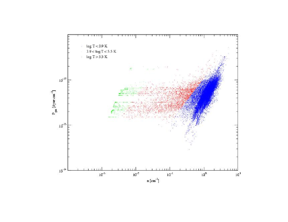
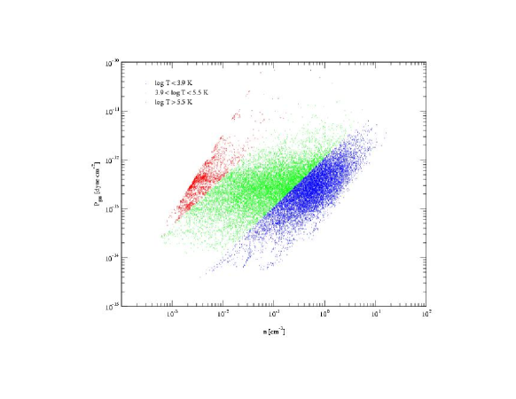
Figure 4: Scatter plot of pressure vs. density for the stratified models, showing every fourth point in the plane of the galaxy, with (a) the Galactic SN rate (model S2), and (b) ten times the Galactic SN rate (model S4). A wide variation of pressure is found for each density. Cool gas with $\log T<3.9$ is shown in blue, warm gas with $3.9<\log T<5.5$ in green, and hot gas with $\log T>5.5$ in red.

A separation between dynamical and thermal timescales is also seen in the stratified hydrodynamical models (Fig. 4. However, these did not include an explicit heating term, but rather had a sharp drop in the cooling rate around $10^{4}$ K, as found in the Dalgarno & McCray (1972) cooling curves. Below that temperature, the cooling timescale was longer than the dynamical timescale rather than shorter, so not much gas had time to cool below it.

The lower boundary of the heavily occupied region on the pressure-density plane appears to be determined by the polytropic behavior of the gas near this cutoff. Fitting to its slope yields values of the polytropic index $\gamma\sim$ 0.6–0.7 in the magnetized model, where a cooling curve increasing as a power law (roughly $T^{2.9}$ can be fit) is balanced by heating, while the slope is much closer to $\gamma\sim$5/3 in the stratified model, where cooling drops fairly abruptly at a certain temperature, and the bulk of the gas at that temperature behaves adiabatically.

Points lying below and to the right of this cutoff line at low pressures and high densities appear to be governed by two different physical mechanisms. In the absence of magnetic fields or heating, but the presence of a low rate of cooling, gas that has been undisturbed for long enough continues to slowly cool, drifting to the right of the line. These points are seen in Figure 4. Low pressures to the left of the line where cooling cuts off in the stratified model also appear, at low to intermediate densities of $10^{-2}$–$10^{-1}$ K cm^-3. These are due to rarefaction waves generated by the turbulent flow acting in gas that is still cooling or has cooled. In the MHD case, some gas becomes magnetically supported, dropping to very low thermal pressures at intermediate densities. As we will show next, this gas does not have low total pressure, only low thermal pressure.

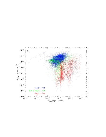
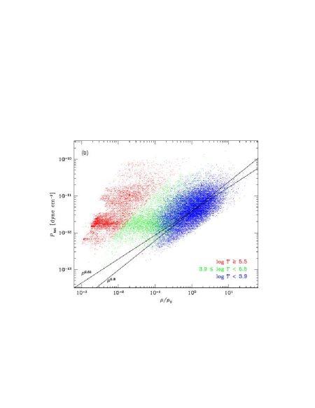
Figure 6: Scatter plot of (a) magnetic vs. thermal pressure and (b) total pressure vs. density at $t=6.6$ Myrs in the MHD simulation, with lines of varying slopes given for comparison to the lower temperature cutoff. We again plotted a subset of $32^{3}$ points sampled at intervals of four points in each direction. Note that regions of very low thermal pressure have substantial magnetic pressures. The total pressure vs. density resembles the hydrodynamic results more strongly than the thermal pressure vs. density plots.

The relation between magnetic and thermal pressure is shown in Figure 6. In Figure 6(a), the relative strength of thermal and magnetic pressure is shown at one time for the magnetized simulation. The scattering of regions at very low thermal pressure all have substantial magnetic pressures, demonstrating that magnetically supported regions can occur. However, their relative importance is rather low, as shown by the small number of points in that regime. Hot gas can be seen, on the other hand, to be dominated by thermal pressure, with low magnetic pressures. In Figure 6(b), the total pressure is shown as a function of density for the same zones. Using total pressure, a clear cutoff at high densities and low pressures is now plain to see, showing that the previous scatter of points beyond it was due to the small magnetically supported regions.

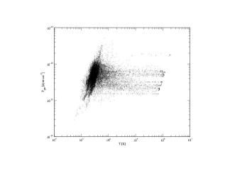
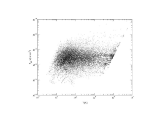
Figure 7: Scatter plot of pressure vs. temperature for a every fourth point in the plane of the galaxy at a time of 60 Myr for (a) the galactic SN rate (model S2), and (b) ten times the Galactic rate (model S4). Note that the pressure scale is substantially broader in plot (b).

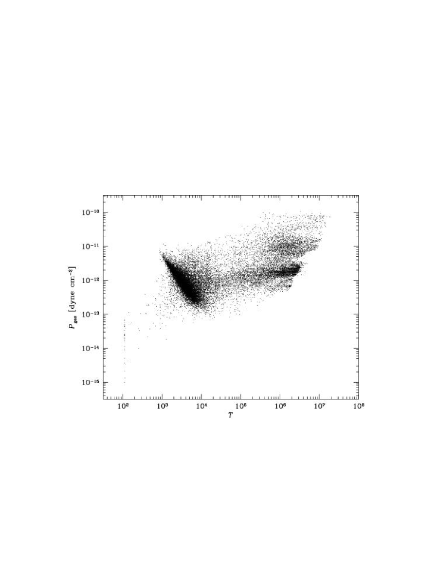
Figure 8: Scatter plot of pressure vs. temperature at $t=6.6$ Myrs in MHD model M2, again showing a subset of $32^{3}$ points sampled at intervals of four points in each direction.

Finally, let us directly consider the distribution of pressures in gas at different temperatures. In Figures 7 and 8 we show scatter plots of thermal pressure against temperature. We note the concentration of points at temperatures below $10^{4}$ K, which once again reflect gas tending to pile up at the drop in the cooling curve or in thermal equilibrium at a wide variety of pressures. The tilt to the right of the cutoff in Figure 7 again indicates $\gamma>1$, with gas at higher pressures also having higher temperatures, while the tilt to the left in Figure 8 indicates $\gamma<1$, with higher pressure gas typically having lower temperatures. Individual SNRs with roughly constant pressures are visible as stripes in the higher temperature regions of the plots. As they cool, they also expand to lower pressures.

4.3 Model Probability Distribution Functions

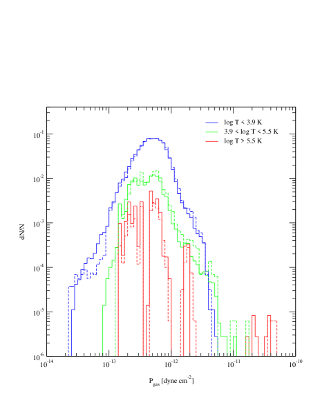
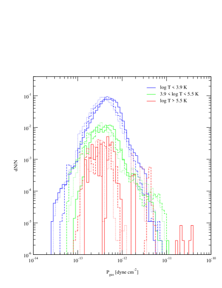
Figure 9: Volume-weighted PDFs of pressure from the stratified models for cool gas with $\log T<3.9$ (blue), warm gas with $3.9<\log T<5.5$ (green), and hot gas with $\log T>5.5$ (red) at (a) resolutions of 1.25 pc (solid, model S2) and 2.5 pc (dashed, model S1) at a time of 60 Myr, and (b) different times of 60 (solid), 70 (dashed), and 80 Myr (dotted) in the 1.25 pc resolution model S2. This model has a galactic rate of SNe.

As we have shown, both the magnetized and the hydrodynamical models have broad ranges of pressures. We can quantify this by examining the pressure PDF, as shown in Figures 9 and 10. In both cases, these show roughly log-normal pressure PDFs, very unlike the power-law distributions predicted by the analytic theory derived by MO, as described in § 3.1. The observed distributions rather more resemble the pressure distributions suggested by PV98, as discussed in § 3.2. Not only is the total distribution broad, even at the Galactic SN rate (Fig. 9), but so is the distribution for different components of the interstellar medium individually. Furthermore, the typical or median pressure at the center of the PDF can vary with temperature, as demonstrated by the PDFs of gas at different temperature.

Our results do not appear to depend strongly on numerical resolution as demonstrated in Figures 9(a) and 10(a) although the details of the history of each SNR and the total amount of energy radiated away will certainly depend on the resolution, as well as our neglect of the physics of the conductive interfaces between hot and warm gas.

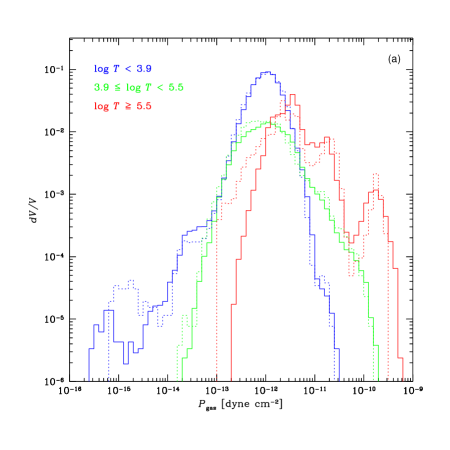
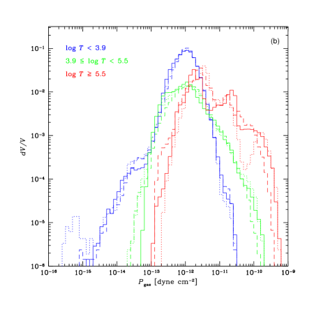
Figure 10: Volume-weighted PDFs of pressure from the MHD models for cool gas with $\log T<3.9$ (blue), warm gas with $3.9<\log T<5.5$ (green), and hot gas with $\log T>5.5$ (red) (a) at different resolutions of 1.6 pc (solid, model M2) and 3.2 pc (dotted, model M1), at a time of 6.05 Myr, and (b) at different times of 5.55 Myr (dashed), 6.06 Myr (dotted), and 6.55 Myr (solid) in the 1.6 pc resolution model M2. This model has twelve times the galactic rate of SNe, which results in a much broader pressure distribution in comparison to Figure 9, whose $x$-axes cover a rather shorter range.

The pressure PDFs also appear to be stable over time, as shown by the comparison of multiple times in Figures 9(b) and 10(b), except for the hot gas, especially at the high-pressure end. At the high SN rate used in Figure 10 individual young SNRs produce discrete bumps that move left towards lower pressures as time passes, eventually merging with the overall distribution, while at the lower SN rate used in Figure 9, individual SNRs remain distinct for longer.

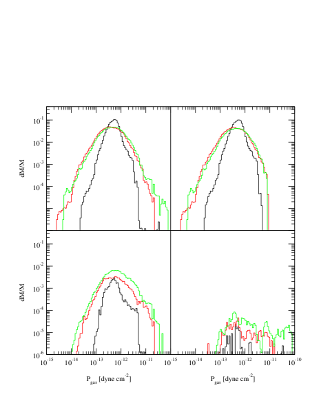
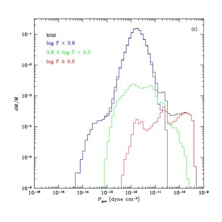
Figure 11: Mass distribution of pressure for (a) the stratified model S1 at a time of 60 Myr for the full distribution (upper left), and for cool gas with $\log T<3.9$ (upper right), warm gas with $3.9<\log T<5.5$ (lower left), and hot gas with $\log T>5.5$ (lower right) at SN rates of 1 (black), 6 (red), and 10 (green) times the Galactic rate, (b) the MHD model M2 for the full distribution (black), and for cool gas with $\log T<3.9$ (blue), warm gas with $3.9<\log T<5.5$ (green), and hot gas with $\log T>5.5$ (red) at a time of 6.55 Myrs. In both models, most of the mass is found in cold gas, with a broad distribution around the peak pressure.

The question of how mass is distributed among regions of different pressure becomes important when considering questions such as the potential ram-pressure confinement of molecular clouds. The mass distribution might be expected to markedly diverge from the volume distribution given by the PDFs shown to date, as most of the hot gas resides at very low densities. In Figure 11 we show mass-weighted distribution functions from each high-resolution model. The cold gas dominates the mass-weighted PDF, but it is found at the same wide range of pressures, with roughly the same peak pressure, as was suggested by the volume-weighted PDFs shown earlier. In particular, a substantial fraction of the mass in the cold gas lies at pressures five to ten times higher than the average pressure, even in the absence of self-gravity.

We have run the stratified case with three different SN rates, as shown in Figures 2 and 12. This allows us to quantitatively test how well our results agree with the analytic theory of PV98 for purely isothermal or polytropic turbulence. We fit two different functions to our pressure PDFs. First, we tried a simple log-Gaussian commensurate with the form of equation (7) for an isothermal gas,

$${\cal P}(x)dx=A\exp[-(x-B)^{2}/C^{2}],$$ (12)

where $x=\log_{10}P$ as before. Then we fit a more complex function capturing the predicted behavior of a polytropic gas with polytropic index $\gamma$,

$${\cal P}(x)dx=A\exp\left[-\frac{(x-B)^{2}}{C^{2}}\exp\left\{\frac{(\gamma-1)(x-B)}{\gamma\epsilon}\right\}-D(x-B)\right].$$ (13)

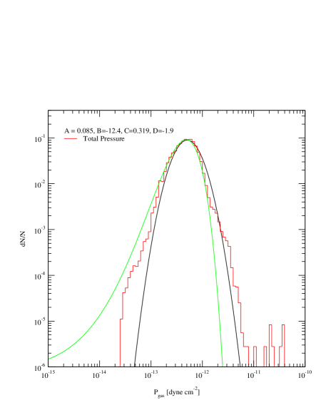
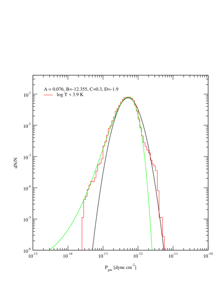
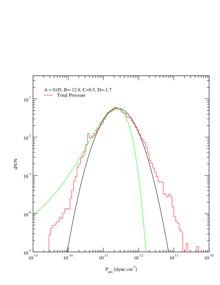
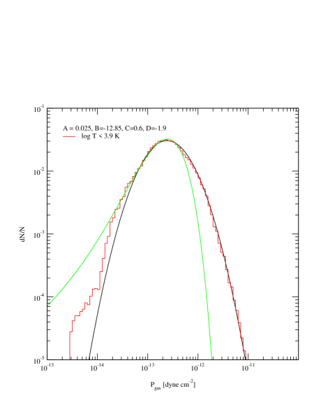
Figure 13: Best fit log Gaussians (black) and tilted log Gaussians following PV98 (green) for the total PDFs (left) and PDFs for cool gas with $\log T<3.9$ (right) for SN rates of (a) Galactic (model S2) and (b) six times Galactic (model S3). The best fit parameters for the tilted Gaussian as described in equation (13) are given in each case.

In both cases, the pressure dispersion is $\sigma_{x}=C/\sqrt{2}$. We find that the value of $\sigma_{x}$ never differs by more than 10% between the Gaussian and the tilted-Gaussian fits. (This can be seen by deriving the tilted Gaussian values from the values of $C$ given in Figure 13.) For simplicity, we therefore use only the Gaussian values in what follows.

We would now like to compare the dispersion $\sigma_{x}$ that we find in our Gaussian fits to the prediction of PV98 given in equation (9). To do this we first need to derive an effective central sound speed $c_{0}$ for our models. As an approximation to $P_{0}$, we take the peak of our fits to the PDFs. This is not quite right, due to the correction factor $s_{0}=-0.5\sigma_{s}^{2}$, but for the relatively low values of $\sigma_{x}$, and thus of $\sigma_{s}$, that we find in these models, it is probably good enough. We then find $\rho_{0}$ and $\gamma$ from the ridgeline at low temperature of the distribution of points in the pressure-density plane (Figs. 4 and 5), roughly following the temperature where the cooling drops sharply in the stratified hydrodynamical case, and the thermodynamic equilibrium curve in the MHD case. This procedure gives $c_{0}\simeq 3$ km s^-1 for the stratified models (corresponding to a temperature of $10^{3}$ K and adiabatic behavior with effective $\gamma=5/3$), and $c_{0}\simeq 6$ km s^-1 for the MHD case (using the effective $\gamma=0.6$ from the slope of the curve).

We then use the rms velocities of each model, which we will discuss in more detail in future work, to predict $\sigma_{x}$. In Table 1 we first compare the fits to the widths predicted by the rms velocity for the full PDF, $\sigma_{x}(\mbox{total})$. The fits to the computational results are factors of five to ten narrower than expected based on the rms velocity. We then compared the computed width of the PDF for only the cool gas with $\log_{10}T<3.9$ to the prediction based on the rms velocity of the cool gas, $\sigma_{x}(\mbox{cool})$. Here, the agreement for the Galactic SN rate is excellent (although the numerical agreement is surely accidental), and it only gradually degrades at higher driving rates.

The grounds for the strong disagreement between the fit and predicted $\sigma_{x}(\mbox{total})$ seem pretty clear. The high-velocity, high-temperature gas is associated with young SNRs and thus has not been fully incorporated into the turbulent flow. The remaining disagreement for the cold gas $\sigma_{x}(\mbox{cool})$ also has several possible explanations: we are not using a polytropic equation of state; our models are three-dimensional instead of one-dimensional; and the distinction between the fully turbulent gas and the more laminar young SNRs is not simply one of temperature. Which of these explanations is most important is less clear. Nevertheless, we may conclude that the rms Mach number of the cold gas does provide a pretty reasonable first guess to the distribution of pressures in the cold gas through equation (9).

5 Comparison to Observations

5.1 Ionized and Atomic Gas

Evidence for a broad distribution of interstellar pressures had already been noted as early as the work on excited levels of Ci by Jenkins & Shaya (1979) and Jenkins et al. (1983). The point was sharpened with the direct comparison of nearby pressures by Bowyer et al. (1995), who compared the pressure of the interstellar medium impinging on the heliosphere with the pressure of the interstellar medium averaged over a 40 pc line of sight as measured with the Extreme Ultraviolet Explorer. Very recently, Jenkins & Tripp (2001) have used the STIS to extend the work on Ci with better resolved data, concluding that the pressure varies by over an order of magnitude both above and below the average value in a small fraction of the gas. Our models naturally explain these variations in the context of a SN-driven interstellar medium. We will endeavor to make a more quantitative comparison soon.

Jenkins et al. (1983) compared their results to the analytic theory of MO, described above in § 3. They found a substantially greater column density of low-pressure material than that predicted, and rather less high-pressure material. As the analytic theory could not predict pressures much less than average, while our models show a broad range of rarefaction waves producing a log-normal pressure distribution around the mean, the low-pressure results appear consistent. Jenkins et al. were observing emission from excited states of Ci in low-temperature gas. We find that much or most of the high-pressure gas resides in the hot medium, so, although we do predict a greater total volume of high-pressure gas than was predicted by MO, we expect that most of it would have been ionized, and therefore not observable by Jenkins et al. (1983), explaining their low column densities of high-pressure material.

Bowyer et al. (1995) compared the pressure they derived from extreme ultraviolet emission along a line of sight to an IRAS detected H i cloud that was determined to be 40 pc away using photometry of stars superposed on the cloud boundaries. They found a pressure of $P/k=$19,000 K cm^-3 for the hot medium, with an absolute lower limit of $P/k=$7,000 K cm^-3. They compared this to the value for the pressure in the Local Cloud of 700–760 K cm^-3 derived by Frisch (1994) from scattering of solar He i 584Åradiation from helium flowing in from the cloud through the heliosphere. McKee (1996) argues that a more careful treatment of the unknown ionization fraction could lead to a local pressure a factor of three higher, reducing, but not eliminating, the discrepancy. We find greater than order of magnitude variations in our models, with pressures reaching values as low as a few hundred K cm^-3 in isolated regions in both sets of models. Interestingly, the lowest pressures are reached at moderately low densities of order 0.1, while the density derived for the Local Cloud by, for example, Quemerais et al. (1994) is 0.14 cm^-3.

An example of a region in the hydrodynamical simulations with high and low pressure regions intertwined in the manner suggested by Bowyer’s observations is the superbubble seen in Figure 1 in the region $200<X<500$ and $100<Y<300$. In this region, even local pressure equilibrium is lacking on scales of tens of parsecs, in contrast to all multi-phase models. Similar regions form regularly over time. In the MHD simulations, an example of a magnetically supported cold cloud in a hot bubble can be seen in the bottom right corner, showing that the explanation advanced by McKee (1996) is also viable, though not unique.

Jenkins & Tripp (2001) found that their results implied an effective polytropic index in the cold gas of $\gamma>0.9$, somewhat higher than the $\gamma=0.72$ derived by Wolfire et al. (1995) for this gas. The suggestion advanced to explain this is that the regions being compressed may be smaller than the cooling length scale, and so may begin to behave adiabatically. An alternative explanation may be drawn from the broad range of pressures at which gas cools in our model: the (relatively sudden) pressurization may happen prior to cooling, rather than to already cooled gas, as required by the derivation of $\gamma$ by Jenkins & Tripp.

The high pressures produced by turbulence in our models also may help elucidate the origin of the opacity fluctuations seen in both H i (Dieter, Welch, & Romney 1976; Diamond et al. 1989; Faison et al. 1998) and metal lines (Meyer & Blades 1996; Watson & Meyer 1996; Lauroesch et al. 1998, Meyer & Lauroesch 1999). These fluctutions were described by Heiles (1997) as tiny-scale atomic structure at overpressures of one to two orders of magnitude to average pressure of the cold gas, which he took to be roughly $P/k=4400$ K cm^-3. Deshpande (2000) suggested that they were due to the spectrum of rather smaller density fluctuations at all scales observed to be produced by the interstellar turbulence. The high pressures we observe in a small fraction of the interstellar gas, in combination with the turubulent structure seen, appear qualitatively consistent with these explanations. Quantitatively distinguishing between them will require a more careful treatment of the cold gas physics and radiative transfer, which we defer to future work. We do note that computations of supersonic isothermal turbulence yield structure functions qualitatively consistent with those required by Deshpande (Mac Low & Ossenkopf 2000; Ossenkopf & Mac Low 2001).

5.2 Molecular Gas

Molecular clouds are observed to have broad linewidths suggesting that they are subject to pressures as high as $10^{5}$ K cm^-3. Larson (1981) was one of the first to suggest that the effective pressure was due to the self-gravity of the cloud. Since then, several authors have found that most of the individual clumps in molecular clouds are not in hydrostatic balance between turbulent pressure and self-gravity, but rather are confined by an external pressure (Carr 1987; Loren 1989; Bertoldi & McKee 1992). The explanation offered for this by Bertoldi & McKee (1992) was that the entire cloud was still subject to self-gravity, even though individual clumps were not, and so the effects of self-gravity on large scales produced pressures that confined the clumps.

In our models, we find pressures in high-density regions of order $10^{5}$ K cm^-3 in the absence of self-gravity, as shown in Figures 4 and 5. These pressures are sufficient to confine observed clumps without invoking self-gravity, suggesting that observed molecular clouds may be primarily pressurized by the ram pressure of the turbulent flows in which they are embedded rather than being self-gravitating objects. Simulated observations of turbulent flows appear to suggest that mass-linewidth relations thought to indicate that they are in virial equilibrium may actually be due to the turbulence itself, or the properties of the observations (Vazquez-Semadeni, Ballesteros-Paredes, & Rodriguez 1997; Ossenkopf, Ballesteros-Paredes, & Heitsch 2001).

Ram pressure is a double-edged sword, however, that can destroy clouds as easily as creating them. This is consistent with the suggestion that they are transient objects with lifetimes of under $10^{7}$ yr first made by Larson (1981), and recently emphasized by Ballesteros-Paredes, et al. (1999a) and Elmegreen (2000). Relying on ram pressures rather than self-gravity to confine observed clumps in molecular clouds would also be consistent with the results of simulations of hydrodynamical and MHD driven, self-gravitating, isothermal turbulence that showed self-gravity only acting on small scales, with turbulent flows dominating the large scales (Klessen et al. 1999; Heitsch et al. 2001). The same flows that confine and destroy the clumps also drive the turbulence observed within them, as the background flow stretches, twists, forms, and destroys dense regions contained within it.

We note that the simple prescriptions we use for cooling below $10^{5}$ K, where non-equilibrium ionization effects become important, and more especially below $10^{4}$ K, where thermal instability is physically expected to be present, are not realistic enough for us to have any degree of confidence in the exact amounts of cold gas produced at any given pressure. However, our qualitative results, produced with two rather different sets of physics, appear quite robust, so we expect future work to refine the details rather than substantially change our picture of molecular clouds forming in transient, high-pressure, high-density regions produced by a supersonic, turbulent flow.

6 Summary

We have examined the distribution of pressures predicted from two different sets of three-dimensional simulations of a SN-driven ISM. In one case we included the effects of vertical stratification, while in the other we included a rather strong magnetic field and a distributed heating function. In all the simulations we examined, we found a broad distribution of pressures over more than an order of magnitude. In the cool gas, with $\log T<3.9$, the probability distribution function of pressure takes a roughly log-normal form with the width of the distribution proportional to the rms Mach number of the cool gas. This form can be derived from the work of PV98 on density distributions, and markedly differs from the power-law distribution predicted by previous work. The higher the SN rate, the broader is the variation of pressures from the mean in both high and low directions.

The only isobaric regions are the interiors of young SNRs; these are also the only laminar flow regions in an otherwise turbulent environment. Most of the mass is in the turbulent gas, however, as is most of the volume even in models driven with ten times the Galactic supernova rate (although questions of the relative strengths of physical turbulent mixing and numerical diffusion will have to be resolved before this conclusion is secure).

We find a broad range of pressures, and a substantial fraction of associated densities far from the thermal equilibrium values. This limits the predictive usefulness of phase diagrams based on thermal equilibrium, although thermal equilibrium at the local pressure will still be the mildly favored state. Gas pressures appear to be determined dynamically, and individual parcel of gas seeks local thermal equilibrium at the pressure imposed on it by the turbulent flow. as suggested by previous authors, the phase diagram is only locally valid. Isobaric thermal instability in such an environment will lead to regions of the phase diagram being mildly disfavored, but no more. Vázquez-Semadeni et al. (2000) and Gazol et al. (2001) used two-dimensional simulations with more physically-motivated cooling curves at lower temperatures to conclude that the effects of the thermal instability will be barely visible in the overall probability distribution functions.

Our results appear consistent with observations that have repeatedly shown the ISM not to be isobaric, including those by Jenkins & Shaya (1979), Jenkins, Jura & Loewenstein (1983), Bowyer et al. (1995), and Jenkins & Tripp (2001). They suggest that, although heating and cooling rates remain important for determining the local density and temperature, they will not produce a global multi-phase medium because of the wide range of pressures present and the dynamical processing of the gas. Rather, a more continuous distribution of densities and pressures will always be present.

Inferences that molecular clouds must be gravitationally bound because of their high observed confinement pressures are called into question by these results. Regions with densities approaching the overall densities of GMCs, and pressures an order of magnitude above the average interstellar pressure appear in our simulations even in the absence of self-gravity. This supports recent suggestions that star-forming molecular clouds may be transient, turbulently-driven, objects (Ballesteros-Paredes et al. 1999ab, Elmegreen 2000). (Objects that do gravitationally collapse from large scales as described by Kim & Ostriker (2001) will also form molecular gas, but will quickly form starburst knots in a burst of violent, unimpeded star formation.)

Even in the presence of a field rather stronger than observed for the Milky Way, only small regions become magnetically supported, with magnetic pressures substantially larger than thermal pressures. The exact filling factor of such regions will need to be determined by more physically accurate studies in the future. Low pressure regions are much more frequently formed by turbulent rarefaction waves, however, especially in gas with slightly lower than average density.

Figures

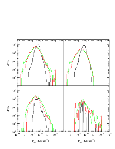
Figure 12: Volume-weighted PDFs of pressure from the stratified models at different SN rates of one (black, model S2), six (green, model S3), and ten (red, model S4) times the galactic rate for the full distribution (upper left), and for cool gas with $\log T<3.9$ (upper right), warm gas with $3.9<\log T<5.5$ (lower left), and hot gas with $\log T>5.5$ (lower right) in the 1.25 pc resolution case.

Table 1: Properties of the models.

			$\Delta x_{\rm min}$	$B_{0}$	Fit			Predicted
model	type	$\tau_{\rm SN}$	(pc)	($\mu$G)	$\sigma_{x}(\mbox{total})$	$\sigma_{x}(\mbox{cold})$		$\sigma_{x}(\mbox{tot})$	$\sigma_{x}(\mbox{cold})$
S1	strat	1	2.5	0	$\cdots$	$\cdots$		$\cdots$	$\cdots$
S2	strat	1	1.25	0	0.22	0.22		0.99	0.22
S3	strat	6	1.25	0	0.35	0.39		4.7	0.52
S4	strat	10	1.25	0	0.39	0.39		5.7	0.61
M1	mhd	12	3.13	5.8	$\cdots$	$\cdots$		$\cdots$	$\cdots$
M2	mhd	12	1.56	5.8	0.32	$\cdots$		2.4	$\cdots$

Table 2: Cooling Times

$\log_{10}T$	$t_{\rm cool}(n/1\mbox{ cm}^{-3})^{-2}$
(K)	(yr)
3	1.7(5)
4	6.0(3)
5	1.6(3)
6	4.4(4)
7	1.2(6)

References

- (1) de Avillez, M. A. 2000, MNRAS, 315, 479
- (2) Ballesteros-Paredes, J., Hartmann, L., & Vázquez-Semadeni, E. 1999a, ApJ, 527, 285
- (3) Ballesteros-Paredes, J., Vázquez-Semadeni, E., & Scalo, J. 1999b, ApJ, 515, 286
- (4) Balsara, D. S. 1998a, ApJS, 116, 119
- (5) Balsara, D. S. 1998b, ApJS, 116, 133
- (6) Balsara, D. S. 2000, Rev. Mex. Astron. Astrof. Ser. Conf., 9, 92
- (7) Balsara, D. S. 2001, J. Comput. Phys., submitted
- (8) Balsara, D. S., & Norton, C. 2001, Parallel Comput., 27, 37
- (9) Balsara, D. S., & Spicer, D. S. 1999a, J. Comput. Phys., 148, 133
- (10) Balsara, D. S., & Spicer, D. S. 1999b, J. Comput. Phys., 149, 270
- (11) Bell, J., Berger, M. Saltzman, J., & Welcome, M. 1994, SIAM J. Sci. Stat. Comput., 15, 127
- (12) Berger, M. J., & Colella, P. 1989, J. Comput. Phys., 82, 64
- (13) Bertoldi, F., & McKee, C. F. 1992, ApJ, 395, 140
- (14) Bowyer, S., Lieu, R., Sidher, S. D., Lampton, M., & Knude, J. 1995, Nature, 375, 212
- (15) Blitz, L., Shu, F. H. 1980, ApJ, 238, 148
- (16) Burkert, A., & Lin, D. N. C. 2000, ApJ, 537, 270
- (17) Cappellaro, E., Turatto, M., Tsvetkov, D. Y., Bartunov, O. S., Pollas, C., Evans, R., & Hamuy, M. 1997, A&A, 322, 431
- (18) Carr, J. S. 1987, ApJ, 323, 170
- (19) Colella, P., & Woodward, P. 1984, J. Comput. Phys., 54, 174
- (20) Cox, D. P., & Smith, B. W. 1974, ApJ, 189, L105
- (21) Dalgarno, A., & McCray, R. A. 1972, ARA&A, 10, 375
- (22) Deshpande, A. A. 2000, MNRAS, 317, 199
- (23) Diamond, P. J., Goss, W. M., Romney, J. D., Booth, R. S., Kalberla, P. M. W., & Mebold, U. 1989, ApJ, 347, 302
- (24) Dickey, J. M., & Lockman, F. J. 1990, ARA&A, 28, 215
- (25) Dieter, N. H., Welch, W. J., & Romney, J. D. 1976, ApJ, 206, L113
- (26) Elmegreen, B. G. 2000, ApJ, 530, 277
- (27) Faison, M. D., Goss, W. M., Diamond, P. J., & Taylor, G. B. 1998, AJ, 116, 2916
- (28) Field, G. B., Goldsmith, D. W., & Habing, H. J. 1969, ApJ, 155, L149 (FGH)
- (29) Frisch, P. 1994, Science, 265, 1423
- (30) Gazol, A., Vázquez-Semadeni, E., Sánchez-Salcedo, F. J., & Scalo, J. 2001, ApJ(Letters), submitted (astro-ph/0105342)
- (31) Heiles, C. 1997, ApJ, 481, 193
- (32) Heiles, C. 2001, ApJ, 551, L105
- (33) Heitsch, F., Mac Low, M.-M., & Klessen, R. S. 2001, ApJ, 547, 280
- (34) Hennebelle, P., & Pérault, M. 1999, A&A, 351, 309
- (35) Hennebelle, P., & Pérault, M. 2000, A&A, 359, 1124
- (36) Jenkins, E. B., Jura, M., & Loewenstein, M. 1983, ApJ, 270, 88
- (37) Jenkins, E. B., & Shaya, E. J. 1979, ApJ, 231, 55
- (38) Jenkins, E. B., & Tripp, T. M. 2001, ApJS, submitted
- (39) Kim, W.-T. & Ostriker, E. C. 2001, ApJ, in press (astro-ph/0105375)
- (40) Klessen, R.S., Heitsch, F., Mac Low, M.-M. 1999, ApJ, 535, 887
- (41) Korpi, M. J., Brandenburg, A., Shukurov, A., Tuominen, I., Nordlund, Å. 1999, ApJ, 514, L99
- (42) Larson, R. B. 1981, MNRAS, 194, 809
- (43) Lauroesch, J. T., Meyer, D. M., Watson, J. K., & Blades, J. C. 1998, ApJ, 507, L89
- (44) Lockman, F. J., Hobbs, L. M., Shull, J. M. 1986, ApJ, 301, 380
- (45) Loren, R. B. 1989, ApJ, 338, 925
- (46) Mac Low, M.-M. 2000, in Stars, Gas, and Dust in Galaxies: Exploring the Links, eds. D. Alloin, K. Olsen, & G. Galaz (San Francisco: ASP), 55
- (47) Mac Low, M.-M., & Ossenkopf, V. 2000, A&A, 353, 339
- (48) MacDonald, J., & Bailey, M. E. 1981, MNRAS, 197, 995
- (49) McKee, C. F. 1996, in The Interplay Between Massive Star Formation, the ISM, and Galaxy Evolution, eds. D. Kunth, B. Guiderdoni, M. Heydari-Malayeri, & T. X. Thuan (Ed. Frontieres: Gif-sur-Yvette, France), 223
- (50) McKee, C. F., & Ostriker, J. P. 1977, ApJ, 218, 148 (MO)
- (51) Meyer, D. M. & Blades, J. C. 1996, ApJ, 464, L179
- (52) Meyer, D. M. & Lauroesch, J. T. 1999, ApJ, 520, L103
- (53) Ossenkopf, V., & Mac Low, M.-M. 2001, A&A, submitted (astro-ph/0012247)
- (54) Ossenkopf, V., Ballesteros-Paredes, J., & Heitsch, F. 2001, ApJ, to be submitted
- (55) Padoan, P. Nordlund, Å, & Jones, B. J. T. 1997, MNRAS, 288, 145
- (56) Passot, T., & Vázquez-Semadeni, E. 1998, Phys. Rev. E, 58, 4501 (PV98)
- (57) Quémerais, E., Bertaux, J.-L., Sandel, B. R., & Lallement, R. 1994, A&A, 290, 941
- (58) Raymond, J. C., Cox, D. P., & Smith, B. W. 1976, ApJ, 204, 290
- (59) Reynolds, R. J. 1987, ApJ, 323, 118
- (60) Roe, P. L., & Balsara, D. S. 1996, SIAM J. Appl. Math., 56, 57
- (61) Rosen, A. & Bregman, J. N. 1995, ApJ, 440, 634
- (62) Shapiro, P. R., & Moore, R. T. 1976, ApJ, 207, 460
- (63) Spitzer, L. 1956, ApJ, 124, 20
- (64) Strange W. G., 1968, SIAM J. Numer. Anal., 5, 506
- (65) Tammann, G. A., Löffler, W., & Schröder, A. 1994, ApJS, 92, 487
- (66) Vázquez-Semadeni, E. 1994, ApJ, 423, 681
- (67) Vázquez-Semadeni, E., Ballesteros-Paredes, J., & Rodriguez, L. F. 1997, ApJ, 474, 292
- (68) Vázquez-Semadeni, E., Gazol, A., & Scalo, J. 2000, ApJ, 540, 271
- (69) Vázquez-Semadeni, E., Passot, T., Pouquet, A. 1995, ApJ, 473, 881
- (70) Vázquez-Semadeni, E., Passot, T., Pouquet, A. 1996, ApJ, 473, 881
- (71) Watson, J. K. & Meyer, D. M. 1996, ApJ, 473, L127
- (72) Wolfire, M. G., McKee, C. F., Hollenbach, D., & Tielens, A. G. G. M., & Bakes, E. L. O. 1995, ApJ, 443, 152