Numerical Simulations of Pinhole and Single Mode Fibre Spatial Filters for Optical Interferometers

Abstract

We use a numerical simulation to investigate the effectiveness of pinhole spatial filters at optical/IR interferometers and to compare them with single-mode optical fibre spatial filters and interferometers without spatial filters. We show that fringe visibility measurements in interferometers containing spatial filters are much less affected by changing seeing conditions than equivalent measurements without spatial filters. This reduces visibility calibration uncertainties, and hence can reduce the need for frequent observations of separate astronomical sources for calibration of visibility measurements. We also show that spatial filters can increase the signal-to-noise ratios of visibility measurements and that pinhole filters give signal-to-noise ratios within 17$\%$ of values obtained with single-mode fibres for aperture diameters up to $3r_{0}$. Given the simplicity of the use of pinhole filters we suggest that it represents a competitive, if not optimal, technique for spatial filtering in many current and next generation interferometers.

1 Introduction

Minimising measurement uncertainties in visibility observations with optical/IR interferometers is one of the major challenges facing any designer of a modern interferometric array. These uncertainties arise from both instrumental and atmospheric effects. The instrumental effects result from aberrations in the optical train and are usually fixed or slowly changing. Atmospheric effects are due to turbulence which causes rapidly-varying phase corrugations in stellar wavefronts. These corrugations corrupt the measured amplitudes and phases of the interference fringes.

The use of the closure phase allows most of the object phase information to be recovered, and closure phase accuracies of a few degrees can be achieved after several seconds of averaging on a bright source. In contrast, the fringe amplitude or visibility is much harder to measure accurately. For example, the mean square visibility of a point source, which ought to have a constant value of 100%, is typically observed to be less than this value and to vary by 10-50% on timescales of minutes to hours. This reduction in fringe visibility is due to mismatches in the shapes of the two wavefronts being interfered, caused by atmospheric and instrumental effects. The atmospheric mismatches vary on millisecond timescales but even the mean effect of these mismatches taken over several seconds varies due to changes in the quality of the seeing.

Some improvement can be obtained by observing a nearby point source and using this to estimate the visibility reduction. However, the use of a calibration source depends on the assumption that the visibility losses remain constant over the several minutes required to switch between calibrator and science objects. This is a poor assumption for atmospheric effects and as a result the calibrated visibilities still show variations at around the 10% level. Furthermore, the constant switching between science and calibration sources dramatically reduces the usable observing time for an interferometer, and hence the amount of science that can be done with an instrument. Thus any system which stabilises the visibility losses is valuable because it can reduce the reliance on a calibration source.

A major step in stabilising visibility losses was made when it was realised that spatially filtering the beams entering the beam combination system would remove the spatial phase perturbations across the incoming wavefronts [1988] and hence remove the major atmospheric contribution to visibility loss. Initial results with this technique have been extremely promising, reducing calibration errors on visibility measurements by as much as two orders of magnitude [1998]. Such high-precision measurements are required for many of the most exciting astrophysical programmes for current and future arrays such as direct measurement of Cepheid pulsation. Consequently spatial filtering is being actively pursued and several interferometer projects are now using or designing spatial filtering systems.

Most of the work on spatial filters has been based on the use of single-mode optical fibres. In this paper we present a detailed analysis of a competing approach, where spatial filtering is provided by focusing a collimated beam onto a pinhole (see Prasad & Loos [1992] and St. Jacques [1998]). Despite the relative simplicity of this approach the use of pinholes has been largely ignored by the astronomical community under the impression that they provide inferior results. Our analysis compares the performance of pinholes and optical fibres under a wide range of conditions. We demonstrate that pinholes represent a simple and effective method of spatial filtering. The use of pinholes instead of optical fibres leads to little loss of performance when used with aperture sizes typical of most current and planned interferometers. We argue that, when the ease of implementation of pinhole systems is taken into account, it is likely that pinhole systems will out-perform fibre systems in practice.

In section 2 we introduce the physical basis for spatial filtering, and we develop our numerical model in section 3. Our simulation and analysis technique is outlined in section 4 and the results are presented and discussed in sections 5 and 6 respectively.

2 Using Pinholes and Single mode optical fibres as spatial filters

2.1 Pinhole spatial filters

Spatial filtering with pinholes is very simple in concept. A lens or mirror is used to focus the collimated beam from a star into the centre of a pinhole which is comparable in size to the diffraction limit of the aperture. The light is transmitted through the pinhole and projected onto another lens to produce a filtered beam which can be interfered with a filtered beam from another telescope. As the electric field distribution at the focus (i.e. the image plane) is simply the Fourier Transform of wavefront across the collimated beam (i.e. the aperture plane), the higher-spatial-frequency perturbations do not pass through the pinhole and the hence the output wavefront is much smoother than that of the input beam.

The visibility of the fringes formed by interfering two such smoothed beams will be higher than it would be for the unfiltered beams and will depend less strongly on the strength of the perturbations in the input wavefront. Smaller pinholes will remove more of the high-frequency wavefront perturbations than larger ones, albeit at the expense of the optical throughput; this trade-off is investigated further in section 4.1.

2.2 Single mode fibre spatial filters

We can replace the pinhole described in section 2.1 with a short length of single-mode fibre to produce a similar effect. The single-mode fibre will reject light which does not match the first guided mode of the fibre [1983]. This mode is approximately Gaussian shaped and is typically of similar size to the diffraction pattern of the aperture being used. The beam leaving the fibre is always the same shape in amplitude and phase, independent of the shape of the input wavefront. For this reason, when the beams emerging from two fibres are interfered there will be no reduction in visibility due to phase corrugation, and hence single mode fibres are often referred to as “perfect spatial filters”. However, there are practical difficulties in efficiently coupling light into single-mode fibres, and these are discussed in section 6.

3 Visibility measurements and auto-calibration

In this paper we concentrate on the effects of spatial filters on the measured fringe visibility and will ignore their effects on closure phases. We define the mean square visibility as the mean squared fringe amplitude normalised by the square of the mean intensity of the fringe. For both pupil-plane and image-plane beam-combination systems, it can be shown [1988] that the mean square visibility will be given by

$$<V^{2}>=\frac{4\Bigl{<}\Bigl{|}\int\limits_{all\vec{r}}A_{1}(\vec{r},t)A_{2}^{\ast}(\vec{r},t)d\vec{r}\Bigr{|}^{2}\Bigr{>}}{\bigl{<}\int\limits_{all\vec{r}}|A_{1}(\vec{r},t)|^{2}d\vec{r}+\int\limits_{all\vec{r}}|A_{2}(\vec{r},t)|^{2}d\vec{r}\bigr{>}^{2}}$$ (1)

where $A_{1}(\vec{r},t)$ and $A_{2}(\vec{r},t)$ denote the instantaneous spatial profiles at time $t$ of the electric fields across the two beams being interfered, $\vec{r}$ denotes a position in the aperture plane and angle brackets denote a mean over $t$. It has been assumed that the fringe amplitude is sampled in a time short compared to the time taken for the wavefront shape to change (the seeing coherence time), but averaged over a period which is long compared to this coherence time.

A useful property of this definition of the visibility is that independent random fluctuations in the overall intensities of the two beams being interfered has no effect on $<V^{2}>$: only differences in the time-averaged beam intensity can cause a reduction in the mean squared visibility [1989]. Such differences in the average will typically be caused by instrumental effects, and we would expect these to vary slowly compared to atmospheric effects.

If the use of spatial filtering reduces the visibility loss due to atmospheric phase perturbations to a negligible level then the measured visibilities (calibrated for instrumental effects) can be taken as the true visibility of the source. This removes the need for frequent switching to a separate calibration source, thereby increasing the useful observing time of the interferometer. Hereafter we will call this technique “auto-calibration”.

4 Technique

4.1 Simulation techniques

We employ a numerical simulation to investigate the performance of the pinhole and fibre spatial filtering systems. Our analysis considers two apertures observing a distant, unresolved, source. We further assume that the light intensity incident on each aperture is equal and that both apertures have identical optical throughputs to a beam combiner which forms interference fringes. We assume the fringe visibility is measured according to equation 1. This simulates observations which would result in unit visibility in the absence of atmospheric effects.

We have assumed that the atmospheric turbulence obeys Kolmogorov statistics with an outer scale much larger than the size of any aperture. We use the technique of McGlamery [1976] to generate random wavefront phase perturbations whose power spectrum is given by [1981]

$$\Phi(\omega)=\frac{0.0229}{r_{0}^{5/3}}\omega^{-11/3}$$ (2)

where $r_{0}$ is the Fried parameter of atmospheric seeing [1966].

Once two random phase screens have been generated they are used to produce two arrays representing the complex electric field amplitudes $A_{1}(\vec{r},t)$ and $A_{2}(\vec{r},t)$ of the two incoming wavefronts. These wavefronts are of constant intensity, i.e. there is no atmospheric scintillation. These arrays are then multiplied by a circular aperture function.

We compensate for the tilt component of the wavefront perturbations in a way that simulates the operation of a fast autoguider. A fast quad-cell wavefront sensor measures the wavefront tilt and adjusts it to equalise the flux in the four quadrants of the image formed by Fourier transforming and squaring the wavefront amplitude. This system of fast guiding is chosen to mimic the auto-guider used at COAST (Baldwin et al. 1994a,b) and many other interferometers such as NPOI [1998] and the VLTI [1990] auxiliary telescope array.

Different amounts of delay in the tip-tilt correction system are simulated assuming a single layer of “frozen” turbulence passing at speed $v$ over each telescope. A guider with a fixed delay $\Delta t$ is simulated by using the tilt correction signal derived from a patch of turbulence offset by $v\Delta t$ from the patch of turbulence used to derive the interferometric signal.

The simulated wavefronts are then spatially filtered using pinholes or single mode fibres. Pinhole spatial filters are simulated by Fourier transforming the wavefront amplitudes to produce the image-plane electric field distribution and then multiplying this distribution by a circular transmission function which is unity inside the pinhole and zero outside it.

For the single-mode fibres we assume a step-index cylindrical core. As the wavefront emerging from the fibre is independent of the incoming beam we need only consider the total amount of light that is coupled into the fibre core. The intensity coupling efficiency of an optical fibre is computed from [1982]

$$\Biggl{|}\int\limits_{\bf\tilde{S}}\tilde{\Psi}_{f}\tilde{\Psi}_{b}{\bf d\tilde{S}}\Biggr{|}^{2}$$ (3)

where $\tilde{\Psi}_{f}$ is the far-field pattern of the the mode propagating inside the fibre and $\tilde{\Psi}_{b}$ is the aperture-plane distribution of the wavefront being focussed on to the fibre end. The electric field patterns ($\tilde{\Psi}_{f}$ and $\tilde{\Psi}_{b}$) have to be normalised such that

$$\int\limits_{\bf\tilde{S}}|\tilde{\Psi}_{f}|^{2}{\bf d\tilde{S}}=\int\limits_{\bf\tilde{S}}|\tilde{\Psi}_{b}|^{2}{\bf d\tilde{S}}=1$$ (4)

We make the approximation that the first guided mode of a step-index fibre is a Gaussian [1988], so that the field distribution in the fibre is given by

$$\Psi_{f}=\sqrt{\frac{2}{\pi}}\frac{1}{w}\exp\Biggl{(}{-\frac{r^{2}}{w^{2}}}\Biggr{)}$$ (5)

where $r$ is the radial distance from the centre of the fibre and $w$ is the ‘Gaussian width’ of the fundamental mode of the fibre. This width is related to the core size of the fibre. The far-field pattern of the fibre is the Fourier transform of this pattern and is therefore also Gaussian.

4.2 Data analysis

The visibility and signal-to-noise ratio (SNR) of an observation are calculated in terms of two intermediate quantities:-

$$\alpha(t)=\Biggl{|}\int\limits_{\mbox{all}\vec{r}}A_{1}(\vec{r},t)A_{2}^{\ast}(\vec{r},t)d\vec{r}\Biggr{|}^{2}$$ (6)

and

$$\beta(t)=\int\limits_{\mbox{all}\vec{r}}|A_{1}(\vec{r},t)|^{2}d\vec{r}+\int\limits_{all\vec{r}}|A_{2}(\vec{r},t)|^{2}d\vec{r}$$ (7)

where $A_{1}(\vec{r},t)$ and $A_{2}(\vec{r},t)$ represent the electric fields across the two wavefronts at some time $t$. The value $\alpha$ represents the instantaneous fringe amplitude and $\beta$ gives the sum of the beam intensities. These values are averaged over a large number (typically between 50 and 3000) of independent random wavefront realisations to reduce their statistical errors.

The visibility we measure (see equation 1) is given by

$$V_{rms}=\sqrt{<V^{2}>}=\sqrt{\frac{4<\alpha(t)>}{<\beta(t)>^{2}}}.$$ (8)

At low light levels (where the fringe measurements are photon-noise-limited and the SNR per sample is much less than unity) the signal-to-noise ratio of the mean squared visibility is given by [1979]:

$$SNR\propto\frac{<\alpha(t)>}{<\beta(t)>}$$ (9)

This signal-to-noise ratio depends on the star brightness and the instrument characteristics, but what we are interested in here is the relative values of the SNR for different spatial filtering configurations and aperture sizes. The values presented here all correspond to measurements using the same number of photons per $r_{0}$-sized patch, where $r_{0}$ is the Fried parameter of the seeing. This implies constant values for $r_{0}$ and the intensity of the source.

4.3 Dimensionless units

In order to make the results of this analysis applicable to a variety of wavelengths, seeing conditions and aperture sizes we express them in terms of two dimensionless units of distance and one of time. In the aperture plane, the aperture sizes are stated as multiples of the Fried parameter, $r_{0}$.

In the image plane of a lens of focal length $f$, the dimensionless unit of length is related to an actual distance, $x$, by $\displaystyle\frac{xD}{f\lambda}$ where $D$ is the beam diameter and $\lambda$ is the wavelength of the light. Using this system the size of the diffraction limited focal spot is independent of primary beam size and wavelength: the radius of the first Airy dark ring will always be 1.22 dimensionless units.

Guider delays are measured in terms of the atmospheric coherence time $t_{0}=0.31r_{0}/v$ where $v$ is the effective wind speed.

5 Results

We present our results for both pinhole and single-mode fibre filters and compare them to results for telescopes without spatial filtering. We consider the effect of filtering on the signal-to-noise ratio of visibility observations and then analyse the visibility loss associated with a pinhole filter.

5.1 Signal-to-noise ratios

Figure 1: Signal-to-noise ratio for pinhole (upper plot) and fibre (lower plot) filters of various filter and aperture sizes. A constant value of the Fried parameter, $r_{0}$, is assumed. All sizes are given in dimensionless units (see section 4.3). The highest contours are 4.75 and 7.25 for pinholes and fibres respectively. Vertical lines show the values of filter size chosen for all further investigations.

Figure 1 shows the signal-to-noise ratio of visibility measurements for a range of pinhole diameters and fibre core radii, assuming no guider delay. By finding the maximum values on these plots we can optimize the filter and aperture size of a telescope for use with either spatial filtering system. For any given aperture size we can find an optimum diameter of pinhole or fibre core radius for which the signal-to-noise ratio is maximised. By inspection we can see that this optimum size varies little with aperture size and so for reasons of clarity we shall henceforth use a single spatial filter size for all aperture sizes. We chose to use pinhole filters with a radius of 1.0 dimensionless unit (see section 4.3) and fibres with Gaussian width (see section 4.1) of 0.75 units for subsequent calculations. These values are shown on figure 1 as vertical lines. For the fibre filter, the absolute peak value of the SNR lies just off the line but we have chosen the line to be optimal for smaller apertures.

Figure 2: The signal-to-noise ratio of a mean squared visibility measurement using optimized fibre and pinhole filters (see section 5.1). Results are shown for circular apertures of various diameters with perfect guiding (see section 4.1).

Figure 2 shows a 1-d section taken along the marked lines in figure 1, along with a comparison with the SNR for beams with no spatial filtering. Clearly there is an advantage in using spatial filtering to increase the signal-to-noise ratio for any set of apertures larger than 1.4$r_{0}$ in diameter. The performance of the two spatial filtering systems is similar for aperture diameters up to $3r_{0}$. At this point the difference in SNR is less than 17$\%$.

The figure also confirms the earlier results that the optimal signal-to-noise ratio is achieved for aperture diameters of 2.8$r_{0}$ [1988] and 6$r_{0}$ [1994] for unfiltered and fibre filtered beams respectively, and demonstrates that the optimal SNR for pinhole filters is reached at around $4r_{0}$. This assumes a fixed photon rate per $r_{0}$-sized patch.

We have repeated this analysis for several values of guider delay and found that, while increasing the guider delay does reduce the signal-to-noise ratio, both filtering systems suffer a similar level of SNR reduction as for an unfiltered telescope.

5.2 Visibility measurements and visibility loss

Figure 3: The root mean squared visibility measured for a point source at various aperture sizes. Results for interferometers incorporating fibre spatial filters, pinhole spatial filters and no spatial filter are presented.

We would expect that there would be no visibility loss for interferometers using fibre spatial filters because fibres are perfect spatial filters. Pinholes are not perfect spatial filters, consequently there will be some residual phase corrugation for any finite sized pinhole. This will result in a reduction of the measured visibility. Figure 3 shows the visibility of a point source measured with a fibre spatial filter, a pinhole spatial filter and no spatial filter for a range of normalised aperture diameters. For the unfiltered system, the degree of visibility loss depends strongly on the ratio of the beam size to the seeing coherence scale. In contrast pinholes filters show significantly less variation in fringe visibility and the visibility measured with fibre based filters is unaffected by seeing.

Figure 4: The root mean squared visibility measured for a point source at various aperture sizes and guider delays using a pinhole filter. Guider delays are given in multiples of the coherence time, $t_{0}$. Error bars are given as standard errors due to statistical uncertainties.

The larger these variations in visibility measurement are for a given change in seeing conditions, the more frequently we will have to switch between sources. If the aperture diameter $D$ remains fixed and the seeing scale $r_{0}$ changes so that $D/r_{0}$ changes from 2 to 3, the measured visibility on a point source for an unfiltered system changes from 0.65 to 0.45, i.e. a fractional change of 30%. Over the same range of seeing conditions the visibility measured with a pinhole filter will vary by 2.5%, in fact over the range $r_{0}\leq D\leq 3r_{0}$ there is a variation of less than $4\%$. This range is comparable to the largest typical variation in seeing during one night and hence suggests that we may only need to make calibration observations once or twice per night, i.e. auto-calibration.

Figure 4 shows the visibility of a point source measured using a pinhole filtering system for a range of seeing conditions and guider delays (note the large difference in vertical range between figures 3 and 4). With a fixed guider delay, if $t_{0}$ changes there can be a greater reduction in measured visibility than is caused by a change in the value of $r_{0}$. However it is usually possible to measure the value of $t_{0}$ from the interferometric data [1997] and therefore allow for this change. This means that pinhole filters can be used for auto-calibration for the majority of seeing conditions.

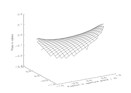
Figure 5: Typical wavefronts from a circular aperture after passing through a pinhole spatial filter. The upper plot shows a wavefront produced with an aperture diameter of $2r_{0}$ whereas the lower plot was produced with an aperture diameter of $5r_{0}$.

An interesting point to consider is why the visibility measurements drop off for pinhole filters at aperture sizes greater than $4r_{0}$. We might naively believe that the tip-tilt correction system compensates for the low spatial frequency wavefront errors and the pinhole removes the high spatial frequency components and therefore the visibility should be independent of seeing for a fixed pinhole size. This is shown to be a poor assumption by inspecting typical wavefronts leaving our simulated filter. Figure 5 shows two such sample wavefronts which have significant tilts that are larger for poorer seeing. This is because the tilt which the guider removes contains contributions from all spatial frequencies and hence is not the same as the tilt for the filtered beam. This leaves a residual tilt in the unfiltered beams which causes a reduction in the measured visibility. This problem could be overcome by a second level of auto-guiding but this would probably involve a reduction in overall optical throughput.

6 Discussion

Our results show that both pinhole and fibre spatial filtering systems dramatically reduce the amount by which the visibility changes with a given change in seeing. For the seeing conditions given in section 5.2, the resistance of the visibility measurements to fluctuations in the level of the seeing is increased by a factor of more than 10 when a pinhole spatial filter is used. Thus it is practical to consider making significantly fewer measurements of a calibration source, perhaps only a few times per night.

The visibilities measured in a system incorporating a fibre spatial filter are in theory completely immune to changes in the seeing. This might be interpreted as meaning that no calibration is required. However, in practice visibility errors would be introduced by any asymmetry in the mean coupling of light from the two arms of the interferometer into the fibres. Such asymmetries could be introduced, for instance if the effectiveness of the autoguiders in correcting the wavefront tilt was different at the two telescopes. Other effects such as the fringes moving during the integration time over which they are measured could also be expected to cause visibility changes at the few percent level. Thus we would still expect some calibration to be necessary with fibre spatial filters.

We have shown that pinhole filters can improve the signal-to-noise ratio of visibility measurements in optical interferometers compared to systems with no spatial filtering. For a fixed photon rate per $r_{0}$-sized patch, a factor of 2 improvement in SNR is achievable with pinholes. For $D\leq 3r_{0}$ there is little difference between the performance of pinhole and fibre filter systems, but fibre filters can give a significantly higher signal-to-noise ratio for $D>3r_{0}$; the highest SNR for a fibre filter is nearly 50% greater than that for a pinhole filter.

However, we must also take into account the relative ease with which the signal-to-noise ratios computed in these simulations can be achieved in practice. One practical consideration is that the 50% greater signal-to-noise ratio for fibre spatial filters is only achieved by using aperture sizes of around $5r_{0}$ or greater. By comparison most actual interferometric telescopes typically operate with diameters much smaller than this. For example the 1.8m outrigger telescopes at VLTI or Keck represent only $2.4r_{0}$ at K band in arcsecond conditions. At this scale we expect the signal-to-noise ratios obtained with an ideal fibre system to be less than 10% higher than with an ideal pinhole system.

Another consideration is the relative ease of achieving signal-to-noise ratios which are close to those predicted from these numerical simulations. In practice, it is rare to achieve more than 75$\%$ of the theoretical coupling efficiency for a single-mode fibre at optical wavelengths. There are a number of reasons for this. The most straightforward of these is the presence of reflection losses at the two air-glass interfaces involved in a fibre spatial filter. This leads to an 8% loss in light. This loss can be reduced if anti-reflection coatings are deposited on the ends of the fibres, but this is rare in practice. The problem of reflection is exacerbated by errors in accurately cleaving and polishing the fibre ends which lead to extra scattering and wavefront errors.

A more significant reason for excess light losses in practical fibre coupling setups is the fact that any wavefront errors introduced by the lens or mirror focusing the light into the fibre will cause a decrease in coupling. For small wavefront errors, the coupling loss will increase as $\sigma_{\phi}^{2}$ where $\sigma_{\phi}$ is the rms wavefront error in radians. Therefore to get less than 20% coupling loss requires rms wavefront errors of less than $\lambda/14$. Most single-mode fibres are efficiently coupled with beams with an f-ratio of about 5 [1988]. This is a relatively fast focal ratio and so to achieve diffraction-limited focusing of a beam onto a fibre typically requires either multi-lens systems or fast off-axis paraboloid mirrors. Manufacturing and aligning these systems to meet a $\lambda/14$ wavefront error specification represents a formidable challenge in the optical regime. Rohloff and Leinert [1991] showed that the typical throughput of a single-mode fibre spatial filter working at optical wavelengths was around 47% in laboratory conditions, whereas our analysis has assumed the theoretical maximum of 78%. Coudé du Foresto et al [1998] describe a total optical throughput of the FLOUR fibre instrument, which works in the K band, as around 5-10% with good seeing with 45cm apertures. This can be compared to an expected throughput of 44% for perfect optics, assuming arcsecond seeing and 60% detector quantum efficiency.

A similar wavefront tolerance to that of fibre systems is required for efficient “coupling” of light into pinholes, but in the case of pinholes the f-ratio of the beam is constrained only by the size of the pinhole. By choosing a relatively large pinhole, a system with a much larger f-ratio can be used, and this relaxes most of the optical tolerances in the system. The pinhole itself is merely the absence of an opaque material and cannot introduce any further aberrations. So one would expect to approach the theoretical coupling efficiency much more closely with a pinhole spatial filtering system than with a fibre system, and with much simpler optics.

There are several other practical implications of implementing spatial filtering that should be considered by any future designer deciding which system to use. One consideration is that fibre based systems can be incorporated into a beam transport device to guide the light to a convenient position, reducing the number of reflections required at an interferometer. Conversely if the spatial filtering system is to be used as an occasional instrument and not permanently installed then removal of a pinhole filter simply requires moving the pinhole to one side, whereas a fibre has a finite length and consequently requires the entire system to be removed or recalibrated. This problem is exacerbated if the fibre is used for beam transport.

7 Conclusions

We have investigated the use of pinhole spatial filters on optical/IR interferometers to reduce the effects of atmospheric phase perturbations on visibility measurements. We have compared the predicted performance of pinhole filters with single-mode fibre filter and unfiltered interferometers.

Our major conclusions are:

1. Both fibre and pinhole spatial filter systems greatly reduce the effect of changing seeing conditions on visibility measurements, compared to an interferometer without spatial filtering.

2. Both fibre and pinhole spatial filter systems can be used to provide “auto-calibration”, where visibility measurements can be made without the need to make regular observations of a separate calibration source.

3. Pinhole spatial filters can improve the signal-to-noise ratio of visibility measurements on optical interferometers for aperture diameters larger than 1.4$r_{0}$.

4. For aperture diameters less than about $3r_{0}$ there is little difference between the signal-to-noise ratio performance of pinhole and fibre spatial filter systems.

5. Fibre spatial filters give superior theoretical signal-to-noise ratios for aperture diameters greater than $3r_{0}$. However, the extra complexity and coupling losses involved with fibres means that pinhole filters may be a superior solution for many current and future optical interferometers.

In summary any current interferometer could benefit from a pinhole spatial filtering system as a simple but effective way to increase overall performance and reduce measurement uncertainties.

8 Acknowledgements

We would like to thank all of the members of the COAST team for their continued support and input. Special thanks go to Chris Haniff and John Baldwin, and to J. Jeans for illuminating contributions.

References

- [1994a] Baldwin J.E., Boysen R.C., Cox G.C., Haniff C.A., Rogers J., Warner P.J., Wilson D.M.A., Mackay C.D., 1994a, Proc. SPIE, 2200, 112
- [1994b] Baldwin J.E., Boysen R.C., Cox G.C., Haniff C.A., Rogers J., Warner P.J., Wilson D.M.A., Mackay C.D., 1994b, Proc. SPIE, 2200, 118
- [1990] Beckers J.M., Enard D., Faucherre M., Merkle F., di Benedetto, G.P., 1990, in Advanced technology optical telescopes IV, SPIE, Tucson, AZ, p.108
- [1997] Burns D., 1997, PhD thesis, Univ. Cambridge
- [1988] Buscher D.F., 1988, MNRAS, 235, 1203
- [1994] Buscher D.F., Shacklan S.B., 1994, Proc. SPIE, 2201, 980
- [1998] Coudé du Foresto V., Perrin G., Ruilier C., Mennesson B., Traub W., Lacasse M., 1998, Proc. SPIE, 3350, 856
- [1979] Dainty J.C., Greenaway A.H., 1979, J. Opt. Soc. Am., 69, 786
- [1966] Fried D.L., 1966, J. Opt. Soc. Am., 56, 1372
- [1998] Hutter D.J., Elias N.M., Hummel C.A., 1998, Proc. SPIE, 3350, 951
- [1983] Jeunhomme L.B., 1983, Single-mode fiber optics: principles and applications, Marcel Dekker
- [1976] McGlamery B.L., 1976, Proc. SPIE, 74, 225
- [1992] Prasad S., Loos G., 1992, in ESO Conference on high resolution imaging by interferometry II, Garching bei München, Germany, 1057
- [1981] Roddier F., 1981, in Wolf E. ed., Progress in optics XIX, North-Holland, 281
- [1991] Rohloff R.-R., Leinert Ch., 1991, App. Opt., 30, 5031
- [1998] St.Jacques D., 1998, PhD thesis, Univ. Cambridge
- [1989] Shaklan S.B., 1989, PhD Thesis, Univ. Arizona
- [1988] Shaklan S., Roddier F., 1988, Appl. Opt., 27, 2334
- [1982] Wagner R.E., Tomlinson W.J., 1982, Appl. Opt., 21, 2671