Weak Lensing and Dark Energy

Abstract

We study the power of upcoming weak lensing surveys to probe dark energy. Dark energy modifies the distance-redshift relation as well as the matter power spectrum, both of which affect the weak lensing convergence power spectrum. Some dark-energy models predict additional clustering on very large scales, but this probably cannot be detected by weak lensing alone due to cosmic variance. With reasonable prior information on other cosmological parameters, we find that a survey covering 1000 sq. deg. down to a limiting magnitude of $R=27$ can impose constraints comparable to those expected from upcoming type Ia supernova and number-count surveys. This result, however, is contingent on the control of both observational and theoretical systematics. Concentrating on the latter, we find that the nonlinear power spectrum of matter perturbations and the redshift distribution of source galaxies both need to be determined accurately in order for weak lensing to achieve its full potential. Finally, we discuss the sensitivity of the three-point statistics to dark energy.

I Introduction

Recent direct evidence for acceleration of the universe Riess ; Perlmutter has spurred considerable activity in finding ways to probe the source of this acceleration, dark energy reconstr ; Weller ; Maor ; Goliath (for a review of dark energy see Ref. Turner_scripta ). Because dark energy varies with redshift more slowly than matter, it starts contributing significantly to the expansion of the universe only relatively recently, at $z\lesssim 2$. This component is believed to be smooth (or nearly so), and therefore detectable mainly through its effect on the expansion rate of the universe. For these reasons, it is generally believed that type Ia supernovae (SNe Ia) and number-count surveys of galaxies and galaxy clusters have the most leverage to probe dark energy, as they probe the distance and volume in the desired redshift range optimal . Indeed, planned supernova surveys (e.g., SNAP ) and number-count methods Holder ; Davis are expected to impose tight constraints on the smooth component; for example, $\sigma(w)\approx 0.05$ from SNAP, assuming a flat universe.

The program of weak gravitational lensing (WL) is primarily oriented toward mapping the distribution of matter in the universe. The paths of photons emitted by distant objects and travelling toward us are perturbed due to the intervening mass. The weak lensing regime corresponds to the intervening surface density of matter being much smaller than some critical value; in that case the observed objects (e.g. galaxies) are slightly distorted. The weak lensing distortions are small (roughly at the 1% level) and one needs a large sample of foreground galaxies in order to separate the lensing effect from the “noise” represented by random orientations of galaxies. Therefore, observations of lensed galaxies provides information on the matter distribution in the universe, as well as the growth of density perturbations. Although the potential of WL has been recognized for around two decades (e.g. early_WL ), only in the 1990s was there a surge of interest in this area Jordi ; Blanford ; Kaiser_92 ; Kaiser_98 ; Jain_Seljak ; Kamionkowski A unique property of WL is that it is sensitive directly to the amount of mass in the universe, avoiding the thorny issue of galaxy-to-mass bias. By measuring ellipticities of a large number of galaxies, one can in principle directly reconstruct the mass density field of an intervening massive object Kaiser_Squires . Indeed, the mass reconstruction of galaxy clusters has been successfully performed on a number of clusters (for a review, see Ref. Mellier ).

An exciting recent development, relevant to this work, was the discovery of weak lensing by large-scale structure, announced by four groups Wittman ; Bacon ; vW ; Kaiser_00 . The results are in mutual agreement and consistent with theoretical expectations, which is remarkable given that they were obtained independently. Although current data impose weak constraints on cosmology (e.g., rule out the Einstein-deSitter Universe with $\Omega_{M}=1$), future surveys with larger sky coverage and improved systematics are expected to impose interesting constraints on cosmological parameters.

The goal of this work is to assess the power of weak lensing to constrain dark energy. This analysis therefore complements that of Huterer & Turner optimal , where the efficacy of SNe Ia and number-count surveys was considered. We follow the standard practice of considering dark energy to be a smooth component parameterized by its energy density (scaled to critical) $\Omega_{X}$ and equation-of-state ratio $w=p/\rho$ Turner_White . Dark energy modifies the WL observables by altering the distance-redshift relation and the growth of density perturbations. As discussed in Sec. VI.2, the nonlinear evolution of perturbations also depends on dark energy; this dependence is much more difficult to calculate and needs to be calibrated from N-body simulations. Overall, the dependence of WL on dark energy is somewhat indirect and expected to be weak, especially when degeneracy with other cosmological parameters is taken into account. Nevertheless, we shall show that, provided systematic errors are controlled and theoretical predictions sharpened, WL surveys can be efficient probes of dark energy, comparable to SNe Ia and number-counts. Proposed deep wide-field surveys such as LSST , the aforementioned SNAP, and VISTA will attempt to constrain dark energy through their WL programs, making our analysis particularly timely.

Previous work on parameter determination from WL centered mostly on $\Omega_{M}$ and $\sigma_{8}$, the rms density fluctuation in spheres of $8{\,{\rm h}^{-1}~{}\rm Mpc}$ Bernardeau ; Jain_Seljak ; here $H_{0}=100\,h\,{\rm km/s/Mpc}$ is the Hubble parameter today. Hu and Tegmark Hu_Tegmark , however, used the Fisher matrix formalism to account for all 8 parameters upon which WL depends, and assumed dark energy to be the vacuum energy (therefore, fixed $w=-1$). We use the same set of parameters, with two changes: we add $w$, and, guided by the ever-stronger evidence from the cosmic microwave background (e.g., boom ; DASI ; max ; Wang ), we assume a flat universe. To assess the accuracy of parameter determination, we too use the Fisher matrix machinery, which has proven to be an extremely efficient and accurate way to forecast errors in experiments where observables depend on many parameters.

This paper is organized as follows. In Sec. II we go over the basic formalism and define the notation. In Sections III and IV we concentrate on the convergence power spectrum, and discuss its dependence on dark energy. Section V discusses the power of weak lensing surveys to probe dark energy, while Sec. VI addresses systematic errors that can lead to biases in parameter estimation. In Sec. VII we discuss the dependence of three-point statistics — bispectrum and skewness of the convergence — on dark energy. We conclude in Sec. VIII.

II Preliminaries

In this Section we cover the basic formalism of weak gravitational lensing (for detailed reviews, see Refs. Bartelmann ; Mellier ). We work in the Newtonian Gauge, where the perturbed Friedmann-Robertson-Walker metric reads

$$ds^{2} = -\left(1+2\Phi\right)dt^{2}+a^{2}(t)\left(1-2\Phi\right)\times$$ (1)

$$\left[d\chi^{2}+r^{2}(d\theta^{2}+\sin^{2}\theta d\phi^{2})\right]$$

where we have set $c=1$, $\chi$ is the radial distance, $\Phi$ is the gravitational potential, and $k=1$, $0$, $-1$ for closed, flat and open geometry respectively. We also use the coordinate distance $r$ which is defined as

$$r(\chi)=\left\{\begin{array}[]{cl}(-K)^{-1/2}\sinh[(-K)^{1/2}\chi],&\;\mbox{if}\;\;\Omega_{\rm TOT}<1;\\[2.84544pt] {\chi},&\;\mbox{if}\;\;\Omega_{\rm TOT}=1;\\[2.84544pt] K^{-1/2}\sin(K^{1/2}\chi),&\;\mbox{if}\;\;\Omega_{\rm TOT}>1.\end{array}\right.$$ (2)

where $K$ is the curvature, $\Omega_{\rm TOT}$ is the total energy density relative to critical, and $K=(\Omega_{\rm TOT}-1)H_{0}^{2}$.

Gravitational lensing produces distortions of images of background galaxies. These distortions can be described as mapping between the source plane ($S$) and image plane ($I$) Hu_White

$$\delta x_{i}^{S}=A_{ij}\delta x_{j}^{I}$$ (3)

where $\delta{\bf x}$ are the displacement vectors in the two planes and $A$ is the distortion matrix

$$A=\left(\begin{array}[]{cc}1-\kappa-\gamma_{1}&-\gamma_{2}\\ -\gamma_{2}&1-\kappa+\gamma_{1}\end{array}\right).$$ (4)

Figure 1: The assumed source galaxy distribution $n(z)$.

The deformation is described by the convergence $\kappa$ and complex shear $(\gamma_{1},\gamma_{2})$. We are interested in the weak lensing limit, where $|\kappa|$, $|\gamma|\ll 1$. The convergence in any particular direction on the sky ${\bf\hat{n}}$ is given by the integral along the line-of-sight

$$\kappa({\bf\hat{n}},\chi)=\int_{0}^{\chi}W(\chi^{\prime})\,\delta(\chi^{\prime})\,d\chi^{\prime}$$ (5)

where $\delta$ is the relative perturbation in matter energy density and

$$W(\chi)={3\over 2}\,\Omega_{M}\,H_{0}^{2}\,g(\chi)\,(1+z)$$ (6)

is referred to as the weight function. Furthermore

$$g(\chi) = r(\chi)\int_{\chi}^{\infty}d\chi^{\prime}n(\chi^{\prime}){r(\chi^{\prime}-\chi)\over r(\chi^{\prime})}$$ (7)

$$\longrightarrow {r(\chi)r(\chi_{s}-\chi)\over r(\chi_{s})}$$ (8)

where $n(\chi)$ is the distribution of source galaxies in redshift (normalized so that $\int dz\,n(z)=1$) and the second line holds only if all sources are at a single redshift $z_{s}$. We use the distribution Wittman

$$n(z)={z^{2}\over 2z_{0}^{3}}\,e^{-z/z_{0}}$$ (9)

with $z_{0}=0.5$, which peaks at $2z_{0}=1$ and is shown in Fig. 1. Our results depend very weakly on the shape of the distribution of source galaxies (assuming this distribution is known, of course). In particular, if all source galaxies are assumed to be at $z=1$, the parameter uncertainties change by at most $\sim 30\%$ percent. Similarly, the distribution given by Eq. (9) which peaks at $z=1.5$ would improve the parameter constraints by 20% or less.

Some clarification is needed regarding observability vs. theoretical computability of WL quantities. The quantity that is most easily determined from observations is shear, which is directly related to the ellipticities of observed galaxies (in the weak lensing limit, shear is equal to the average ellipticity). Shear is given by Kaiser_98

$$\gamma_{1}+i\gamma_{2}=\frac{1}{2}\left(\psi_{,11}-\psi_{,22}\right)+i\psi_{,12}$$ (10)

where $\psi$ is the projected Newtonian potential, $\psi_{,ij}=-2\int g(\chi)\,\Phi_{,ij}\,d\chi$, and commas denote derivatives with respect to directions perpendicular to the line of sight. Unfortunately, this quantity is not easily related to the distribution of matter in the universe and the cosmological parameters. Convergence, on the other hand, is given by

$$\kappa=\frac{1}{2}\left(\psi_{,11}+\psi_{,22}\right)$$ (11)

which (in Limber’s approximation) can be directly related to the distribution of matter through the Poisson equation (see Eq. (5)), and is convenient for comparison with theory. However, it is very difficult to measure the convergence itself, as convergence depends on the magnification of galaxies which would somehow need to be measured (although there may be ways to do this; see Ref. Broadhurst ) . Note also that computing the convergence from the measured shear is difficult in general, since the inversion kernel is broad and requires knowledge of shear everywhere Kaiser_Squires . In the weak lensing limit, however, the problem is much easier, since the two-point correlation functions of shear and convergence are identical.

In this work we use power spectrum of the convergence (defined in Eq. (13) below) as the principal observable that will convey information from weak lensing.

III Convergence Power Spectrum

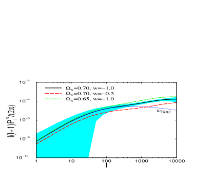
Figure 2: Top panel: The convergence power spectrum for three pairs of ($\Omega_{X}$, $w$). The shaded region represents 1-$\sigma$ uncertainties (corresponding to $\Omega_{X}=0.7$, $w=-1$ curve) plotted at each $l$. The uncertainties at low $l$ are dominated by cosmic variance, and those at high $l$ by Poisson (shot) noise; see Eq. (15). We also show the contribution to $P_{l}^{\kappa}$ from the linear matter power spectrum only. Bottom Panel: $P_{l}^{\kappa}/\Delta P_{l}^{\kappa}$ (“signal-to-noise”) for the convergence power spectrum for each individual $l$.

The convergence can be transformed into multipole space (see e.g. Ref. Bartelmann )

$$\kappa_{lm}=\int d{\bf\hat{n}}\,\kappa({\bf\hat{n}},\chi)\,Y_{lm}^{*}.$$

The power spectrum of the convergence $P_{l}^{\kappa}$ is then defined by

$$\langle\kappa_{lm}\kappa_{l^{\prime}m^{\prime}}\rangle=\delta_{l_{1}l_{2}}\,\delta_{m_{1}m_{2}}\,P_{l}^{\kappa}.$$

Using Limber’s approximation — the fact that the weight function $W$ is much broader than the physical scale on which the perturbation $\delta$ varies — the convergence power spectrum can be written as

$$P_{l}^{\kappa} = \int_{0}^{\chi_{s}}d\chi\frac{W^{2}(\chi)}{r^{2}(\chi)}P(l/r(\chi),z)$$ (12)

$$= {2\pi^{2}\over l^{3}}\int_{0}^{z_{s}}dz\,{W^{2}(z)\,r(z)\over H(z)}\Delta^{2}(l/r(z),z)$$ (13)

where in the second line we assume a flat universe where $d\chi=dr$. Here $P(k,z)$ is the matter power spectrum as a function of redshift $z$, and

$$\Delta^{2}(k,z)={k^{3}P(k,z)\over 2\pi^{2}}$$ (14)

is power per unit logarithmic interval in wavenumber, which we also refer to as the matter power spectrum.

Power spectrum of the convergence is displayed in the top panel of Fig. 2 for three values of ($\Omega_{X}$, $w$) and down to scales of about one arcminute ($l=10000$). The uncertainty in the observed weak lensing spectrum is given by Kaiser_92 ; Kaiser_98

$$\Delta P_{l}^{\kappa}=\sqrt{2\over(2\ell+1)f_{\rm sky}}\left(P_{l}^{\kappa}+{\left<\gamma_{\rm int}^{2}\right>\over\bar{n}}\right)\,,$$ (15)

where $f_{\rm sky}=\Theta^{2}\pi/129600$ is the fraction of the sky covered by a survey of dimension $\Theta$ and $\left<\gamma_{\rm int}^{2}\right>^{1/2}\approx 0.4$ is the intrinsic ellipticity of galaxies. The first term corresponds to cosmic variance which dominates on large scales, and the second to Poisson noise which arises due to small number of galaxies on small scales. Bottom panel of Fig. 2 shows the signal-to-noise $P_{l}^{\kappa}/\Delta P_{l}^{\kappa}$. It is apparent that the bulk of cosmological constraints comes from multipoles between several hundred and several thousand. Wider and deeper surveys widen the range of scales with high signal-to-noise. Note also that the weak lensing power spectrum is relatively featureless because of the radial projection (Eq. (13)). It can be characterized by amplitude (normalization), overall tilt, a “turnover” at $l\sim 100$ which is due to the turnover in the matter power spectrum, and a further increase at $l\sim 1000$ and flattening at $l\sim 10000$ which are due to the nonlinear clustering of matter.

The systematic error in shear measurements ideally needs to be small enough so as not to exceed the statistical error shown in Fig. 2. The maximum allowed systematic error can be estimated using the following argument . The shear variance in circular aperture of opening angle $\theta$ can be written in terms of the convergence power spectrum as Bartelmann

$$\langle\gamma^{2}(\theta)\rangle = 2\pi\int_{0}^{\infty}dl\,lP_{\kappa}^{l}\left({J_{1}(l\theta)\over\pi l\theta}\right)^{2}$$ (16)

$$\approx (2\pi)^{2}\int_{0}^{\infty}{dl\over l}{\cal P}_{\kappa}^{l}\left({J_{1}(l\theta)\over\pi l\theta}\right)^{2}$$ (17)

$$\simeq {\cal P}_{\kappa}^{l=1/\theta}$$ (18)

which is the power in unit logarithmic interval evaluated at $l=1/\theta$ (here ${\cal P}_{\kappa}^{l}=l(l+1)/(2\pi)P_{\kappa}^{l}$). The tightest requirement is on scales of 1 arcmin ($l\approx 2000$), where the fractional uncertainty in power per unit logarithmic interval is about $1/200$. Therefore the RMS of shear on scale $\theta$ is given by

$$\delta\sqrt{\langle\gamma^{2}(\theta)\rangle} \approx \delta\sqrt{{\cal P}_{\kappa}^{l=1/\theta}}$$ (19)

$$= {1\over 2}\sqrt{{\cal P}_{\kappa}^{l=1/\theta}}\left(\delta{\cal P}_{\kappa}^{l=1/\theta}\over{\cal P}_{\kappa}^{l=1/\theta}\right)$$ (20)

$$\simeq {1\over 2}\times\sqrt{10^{-4}}\times{1\over 200}$$ (21)

$$\approx 2.5\times 10^{-5}$$ (22)

$$\lesssim 0.01\sqrt{\langle\gamma^{2}(\theta)\rangle}.$$ (23)

Therefore, the systematic error in individual shear measurements should be less than $1\%$ in order to be subdominant to statistical error — a very challenging requirement indeed!

IV Dependence on dark energy

The sensitivity of the convergence power spectrum to dark energy can be divided into two parts. Dark energy

a) modifies the background evolution of the universe, and consequently the geometric factor $W^{2}(z)r(z)/H(z)$, and

b) modifies the matter power spectrum.

We now discuss each of these dependencies.

IV.1 The lensing weight function

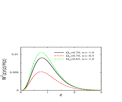
Figure 3: The weight function $W^{2}(z)r(z)/H(z)$ for three pairs of ($\Omega_{X}$, $w$).

Function $W(z)$ is bell-shaped, and has a maximum at $z\approx z_{s}/2$, where $z_{s}$ is redshift of lensed galaxies, indicating that lensing is the most effective at distances halfway between the source and the observer. Since $r(z)$ and $H(z)$ are varying with redshift monotonically and slowly, the function $W^{2}(z)r(z)/H(z)$ will also be bell-shaped with maximum at $z\gtrsim z_{s}/2$. $W(z)$, $r(z)$ and $1/H(z)$ all decrease with increasing $w$, and therefore the total weight decreases. As $\Omega_{X}$ decreases, $r(z)$ and $1/H(z)$ decrease but $W(z)$ increases, and the latter prevails; see Fig. 3. Therefore, changing $w$ ($\Omega_{X}$) makes the normalization and total weight change with the same (opposite) sign, leading to large (small) change in $P_{l}^{\kappa}$ on large scales; see Fig. 2.

IV.2 The Matter Power Spectrum

The matter power spectrum can be written as

$$\Delta^{2}(k,z) = \delta_{H}^{2}\left(k\over H_{0}\right)^{3+n}\!\!T^{2}(k,z)\,{D^{2}(z)\over D^{2}(0)}\,T_{NL}(k,z)$$ (24)

where $\delta_{H}$ is perturbation on Hubble scale today, $T(k)$ is the transfer function, $D(z)/D(0)$ is the growth of perturbations in linear theory relative to today, and $T_{NL}(k,z)$ is the prescription for nonlinear evolution of the power spectrum.

In the presence of dark energy, the matter power spectrum will be modified as follows.

$\bullet$ The normalization $\delta_{H}$ increases with increasing $\Omega_{X}$ and decreasing $w$. This happens because the growth of structure is suppressed in the presence of dark energy, and the observed structure today can only be explained by a larger initial amount of perturbation. We choose to normalize the results to COBE measurements Bennett , and adopt the fit to COBE data of Ma et al. (Ma_QCDM , heretofore Ma QCDM)

$$\delta_{H} = 2\times 10^{-5}\alpha(0)^{-1}\Omega_{M}^{\,c_{1}+c_{2}\ln(\Omega_{M})}$$ (25)

$$\times\exp\left[c_{3}(n-1)+c_{4}(n-1)^{2}\right]$$

where $c_{1\ldots 4}$ and $\alpha_{0}$ are functions of $\Omega_{X}$ and $w$ and are given in Ma QCDM. Since the COBE normalization for $\Lambda$CDM models is accurate to between 7% and 9% Bunn_White ; Liddle_Lyth , we adopt the accuracy of 10% for the dark-energy case.

$\bullet$ The transfer function for cosmological models with neutrinos and the cosmological constant is given by fits of Hu and Eisenstein Hu_transfer , which we adopt in our analysis. These formulae are accurate to a few percent for the currently favored cosmology with low baryon abundance. Dark energy will not directly modify the transfer function, except possibly on the largest observable scales (of size $\sim H_{0}^{-1}$), where dark energy may cluster. This signature can be ignored, as it shows up on scales too large to be probed by WL; we further discuss this in Sec. V.7.

$\bullet$ The linear theory growth function $D(z)=\delta(z)/\delta(0)$ can be computed from the fitting formula for the dark-energy models given in Ma QCDM, which generalizes the $\Lambda$CDM growth function formula of Carroll et al. Carroll . We use this fitting function, noting that its high accuracy ($\leq 2\%$) justifies avoiding the alternative of repeatedly evaluating the exact expression for the growth function (e.g. Peebles , p. 341).

$\bullet$ The last, and most uncertain, piece of the puzzle is the prescription for the non-linear evolution of density perturbations. This is given by the recipe of Hamilton et al. Hamilton as implemented by Peacock and Dodds (PD ; heretofore PD), as well as Ma (Ma_LCDM , heretofore Ma $\Lambda$CDM). These two prescriptions were calibrated for $\Lambda$CDM models, although the PD formula seems to adequately fit models with $w>-1$ (M. White, private communication). Ma QCDM prescription Ma_QCDM , on the other hand, gives explicit formulae for the nonlinear power spectrum in the presence of dark energy (i.e., a component with $w\geq-1$). Unfortunately, we found that the PD and Ma QCDM prescriptions agree (to $\sim 15$%) only at values of $w$ where Ma QCDM was tested. At other values of $w$ the maximum disagreement between the two is up to 50%, and it is not clear which fitting function, if any, is to be used. We choose to use the PD prescription primarily because it is implemented for all $w$ and therefore facilitates taking the derivative with respect to $w$ needed for the Fisher matrix. In Sec. VI.2 we explore the possible parameter biases due to the uncertain calibration of the nonlinear power spectrum.

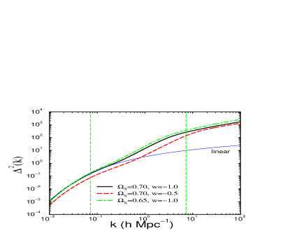
Figure 4: The matter power spectrum at $z=0$ for three pairs of $(\Omega_{X},w)$. Linear power spectrum corresponding to the fiducial spectrum is shown by the thin solid curve. Vertical lines delimit the interval which contributes significantly to the WL convergence power spectrum, roughly corresponding to $100\leq l\leq 10000$. It can be seen that the ability to determine cosmological parameters will depend critically upon the knowledge of the nonlinear power spectrum.

Figure 4 shows the matter power spectrum at $z=0$ for three pairs of $(\Omega_{M},w)$. When $\Omega_{X}$ or $w$ are varied, the growth and normalization change affecting all scales equally. Varying $\Omega_{X}$ also changes the transfer function (at $k\gtrsim 0.02{\,{\rm h}^{-1}~{}\rm Mpc}$). On smaller scales ($k\gtrsim 0.2{\,{\rm h}^{-1}~{}\rm Mpc}$), the non-linear power spectrum is further affected by dark energy.

IV.3 Angular Scale – Physical Scale Correspondence

To illustrate the correspondence between wavenumbers $k$ and multipoles $l$, let us assume the matter power spectrum peaked at a single multipole $k_{1}$

$$\Delta^{2}(k)=\langle\delta^{2}\rangle k_{1}\delta(k-k_{1})$$ (26)

normalized so that $\int\Delta^{2}(k)d\ln k=\langle\delta^{2}\rangle$ (here $\langle\delta^{2}\rangle$ is the auto-correlation function of density contrast in real space). Then, assuming for simplicity that all sources are at a single redshift $z_{s}$, we have

$$l(l+1)P_{l}^{\kappa}/(2\pi)\propto{l^{3}\over k_{1}^{4}}\left(1-{l\over r(z_{s})k_{1}}\right)^{2}$$ (27)

for $l<k_{1}r(z_{s})$, and zero for $l\geq k_{1}r(z_{s})$. The plot of the convergence power spectrum is given in Fig. 5 for two values of $k_{1}$. The multipole power peaks at $l=3/5\,k_{1}r(z_{s})$. Assuming a survey with $z_{s}=1$, the scale at which the non-linear effects become significant, $k\approx 0.2{\,{\rm h}^{-1}~{}\rm Mpc}$, corresponds to $l\approx 300$. Our constraints mostly come from angular scales $l\sim 1000$, corresponding to $k\sim 1{\,{\rm h}^{-1}~{}\rm Mpc}$. The bulk of WL constraints therefore comes from non-linear scales.

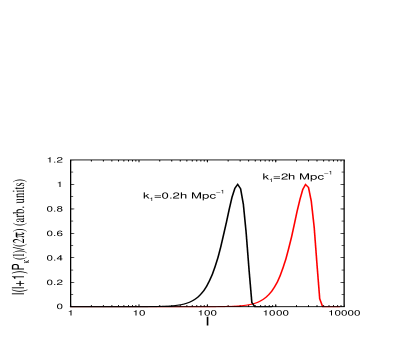
Figure 5: Power spectrum of the convergence assuming matter power spectrum is a delta-function at $k_{1}$, shown for two different values of $k_{1}$. This shows the correspondence between physical and angular scales (for $z_{s}=1$ and our fiducial $\Lambda$CDM cosmology).

V Constraints on Dark Energy

V.1 The Fisher matrix formalism

The fact that the relatively featureless $P_{l}^{\kappa}$ depends upon a number of cosmological parameters directly leads to parameter degeneracies and limits the power of weak lensing to measure these parameters independently of other probes, even for the case of a full-sky survey. To estimate how accurately cosmological parameters can be measured, we use the Fisher matrix formalism Fisher . This method has already been used to forecast the expected accuracies from CMB surveys Zaldarriaga_Seljak ; Eis_Hu_Teg , SNe Ia SN_Fisher ; optimal ; Goliath and number counts Holder_01 and was found to agree very well with direct Monte-Carlo error estimation. Its considerable advantage over Monte Carlo is that it does not require simulations and analyses of data sets, but only a single evaluation of a simple analytic expression. Furthermore, the Fisher matrix formalism allows easy inclusion of Bayesian priors and constraints from other methods.

The Fisher Matrix is defined as the second derivative of the negative log-likelihood function

$$F_{ij} = -\left<\partial^{2}\ln L\over\partial p_{i}\partial p_{j}\right>_{\bf x}$$ (28)

$$= \,\sum_{l}\frac{1}{(\Delta P_{l}^{\kappa})^{2}}{\partial P_{l}^{\kappa}\over\partial p_{i}}{\partial P_{l}^{\kappa}\over\partial p_{j}}\,.$$ (29)

where $L$ is the likelihood of the observed data set ${\bf x}$ given the parameters $p_{1}\ldots p_{n}$. The second line follows by assuming that $L$ is Gaussian in the observable $P_{l}^{\kappa}$, which is a good assumption for small departures around the maximum.

In practice we do not estimate the power spectrum at every multipole $l$, but rather bin $P_{l}^{\kappa}$ in 17 bins. We explicitly checked that binning makes no significant difference in our results (this is not surprising, as the convergence power spectrum doesn’t have features that would get washed out by moderate-resolution binning). We considered $P_{l}^{\kappa}$ at $100\leq l\leq 10000$, corresponding to angles between 1 arcminute and 2 degrees on the sky. Variations in the minimum and maximum $l$ do not change any of our results, as very large and very small scales are dominated by cosmic variance and Poisson noise respectively.

Finally, we need to choose steps in parameter directions when taking numerical derivatives. We choose the steps to be 5% of the parameter values, making sure to take two-sided derivatives.

V.2 The fiducial cosmology and fiducial survey

Finally, we need to choose the fiducial survey, i.e. sky coverage and depth of the survey. We do not consider any single experiment in particular, but rather adopt numbers roughly consistent with proposed dedicated wide-field surveys expected to become operational in several years. We assume a survey covering 1000 sq. deg. down to a limiting magnitude $R=27$; dependence of the results upon these two parameters is discussed in Sec. V.6. Surveys of this power are not yet operational, but are expected in the near future with results perhaps by the end of this decade. To convert from magnitudes to surface density of galaxies, we use the correspondence from Herschel and Hubble Deep Fields Metcalfe , which for our fiducial numbers implies 165 gal/arcmin². We assume that the only sources of noise are statistical: cosmic variance which dominates on large scales, and shot-noise dominant on small scales. We discuss the effect of systematics in Sec. VI.

V.3 Parameter space

Power spectrum of the convergence depends on 7 parameters: $\Omega_{X}$, $w$, $\Omega_{M}h^{2}$, $\Omega_{B}h^{2}$, $\delta_{H}$, $n$, and $m_{\nu}$, where $\Omega_{B}$ is the energy density in baryons (relative to critical), $n$ is the spectral index of scalar perturbations, and $m_{\nu}$ the neutrino mass summed over all species. In addition, $P_{l}^{\kappa}$ depends upon the redshift distribution of source galaxies. Throughout, we use a fiducial model that fits well all experiments so far: $\Omega_{X}=1-\Omega_{M}=0.7$ (flat universe assumed), $h=0.65$, $\Omega_{B}h^{2}=0.019$, $n=1.0$, and $\delta_{H}$ inferred from COBE measurements as described in Sec. IV.2. The mass of neutrino species is quite uncertain, but, according to solar neutrino experiments, likely to be between zero and a few eV; we adopt $m_{\nu}=0.1{\rm eV}$.

We would like to get an insight in parameter degeneracies, in particular between the equation of state ratio $w$ and other parameters. To do that, we compute the correlation between $w$ and other parameters. The correlation coefficient is given by

$$\rho(w,p_{i})={{\rm Cov}(w,p_{i})\over\sqrt{{\rm Cov}(w,w){\rm Cov}(p_{i},p_{i})}}$$ (30)

where ${\rm Cov}(p_{i},p_{j})=F_{ij}^{-1}$ is an element of the covariance matrix. Because imposing priors would alter the covariance matrix and confuse its interpretation, at this point we add no priors except for COBE normalization (10% in $\delta_{H}$) and perfect knowledge of galaxy redshifts.

The most significant correlations are $\rho(w,\Omega_{X})=-0.96$, $\rho(w,\Omega_{B}h^{2})=-0.83$, and $\rho(w,m_{\nu})=0.81$. We find that these and other correlations are typically very dependent on the fiducial model and the assumed prior. Finally, we examine the eigenvalues and eigenvectors of the Fisher matrix. The combination $0.61\,\Omega_{X}+0.21\,w$ is determined to an accuracy of about $0.03$; this is the best-determined combination containing significant components in $\Omega_{X}$ and $w$ directions. The most poorly combination of all is one almost entirely in the $w$-direction: $0.97\,w-0.21\,\Omega_{X}$; it is determined to about 0.4.

V.4 Bayesian Priors

Without any prior information on cosmological parameters, weak lensing imposes very weak constraints on dark energy (and other parameters as well). The reason is that the power spectrum of the convergence is featureless, owing to the fact that it represents the radial projection of the density contrast. Unlike the CMB spectrum, it lacks bumps and wiggles that would help break parameter degeneracies. Constraints rapidly improve, however, if the redshift distribution of source galaxies is known. We assume this to be the case; indeed, photometric redshift techniques already show that distribution of source galaxies in weak lensing surveys will be determined independently of cosmological parameters (e.g., Hogg ). Exact knowledge of the source distribution is obviously a strong and perhaps unrealistic assumption, and in Sec. VI we explore what happens when the uncertainties are included.

There is no reason to expect that any cosmological probe alone should carry the burden of determining all cosmological parameters. Indeed, a number of cosmological parameters are already pinned down quite accurately by other means. In about 10 years, when powerful weak lensing surveys we consider complete their observational programs, parameters inferred from the CMB (such as $\Omega_{M}h^{2}$, $\Omega_{B}h^{2}$ and $n$) will be determined to an accuracy of several percent Eis_Hu_Teg . The neutrino mass, on the other hand, is poorly known today, but in the near future it is likely to be constrained by a combination of CMB, Ly-$\alpha$ forest Ly_alpha , as well as solar and atmospheric neutrino measurements.

For these reasons, we include Gaussian priors on cosmological parameters (other than $\Omega_{X}$ and $w$). We consider two sets of priors, and call them “COBE+photo-z” and “Planck (T)”. The former set of priors is a weak one: we only include the 10% uncertainty in COBE normalization and, as mentioned above, knowledge of the distribution of background galaxies. The latter set is a moderate one, corresponding to the COBE+photo-z prior, plus the constraints expected from the Planck mission with temperature information only (Table 2 of Ref. Eis_Hu_Teg ): $\sigma(\ln\Omega_{M}h^{2})=0.064$, $\sigma(\ln\Omega_{B}h^{2})=0.035$, $\sigma(n)=0.04$, and $\sigma(m_{\nu})=0.58$ . We note, however, that details of the second prior do not change the results much; for example, using the considerably weaker assumptions corresponding to MAP mission (with temperature only) instead of Planck (T), errors in $\Omega_{X}$ and $w$ degrade by only 10% and 5% respectively. Similarly, using the very strong prior of Planck constraints (temperature and polarization) combined with those from Sloan Digital Sky Survey (SDSS ), the constraints improve only by about 20%. The reason for this weak dependence on the prior is easy to understand: by assuming the knowledge of the distribution of source galaxies and adding other priors, we have broken the major degeneracy between $\Omega_{X}$, $w$ and other parameters; further information on other parameters leads to small improvements in the constraints on dark energy.

V.5 Results

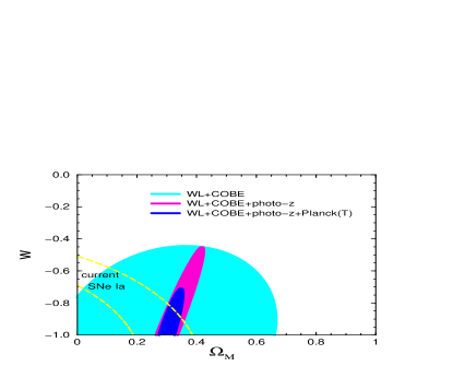
Figure 6: 68% C.L. constraints on $\Omega_{M}$ and $w$ for two values of $m_{\nu}$. We assume a survey of 1000 sq. deg. down to 27th magnitude in $R$-band, assume knowledge of the distribution of source galaxies, and impose the Planck (T) prior on other parameters Eis_Hu_Teg . The strength of the constraints does not depend sensitively on the set of priors, but does depend on the fiducial model (e.g., the neutrino mass). For orientation, current 1-$\sigma$ constraints from 42 type Ia supernovae Perlmutter are also shown.

An example of the constraints that weak lensing can impose on dark energy is shown in Fig. 6. Here we show the 68% constraint regions for our fiducial WL survey (1000 sq. deg. down to 27th mag) with several sets of priors on other parameters. The ellipse is oriented so that increase in $w$ is degenerate with increase in $\Omega_{M}$, which is opposite of what we would expect; this is due to the fact that we assume galaxy redshifts to be known . Table 1 lists the uncertainties using two sets of priors. Weak lensing is potentially a strong probe of dark energy: the 1-$\sigma$ uncertainties in $\Omega_{X}$ and $w$ are $\sim 5\%$ and 20-40% respectively (depending on the set of priors), which is somewhat weaker than statistical errors expected from future SNe Ia and number-count surveys. We emphasize that these numbers are the best ones possible given the survey specifications; systematic errors may weaken the constraints (see Sec. VI). It is also true, however, that weak lensing tomography can significantly improve these constraints (more on that in Sec. V.6).

TABLE 1

Constraints on dark energy Prior COBE + photo-z Planck (T) $\sigma(\Omega_{X})$ 0.08 0.04 $\sigma(w)$ 0.36 0.19

Top panel of Fig. 7 shows the dependence of the uncertainties in $\Omega_{X}$ and $w$ on the sky coverage, holding the depth of the survey fixed at 27th mag. Lower panel of the same Figure shows dependence of the uncertainties on the depth of the survey, holding the sky coverage fixed at 1000 sq. deg. The constraints on $w$ depend quite strongly on the depth of the survey — for example, constraint on $w$ would improve by a factor of two by increasing the coverage of the survey to 5000 sq. deg. The dependence on the depth is also significant, but probably complicated by some practical problems; for example, galaxy overlap. Therefore, future surveys with very deep and/or wide sky coverage will be especially effective probes of dark energy.

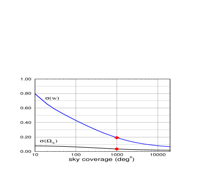
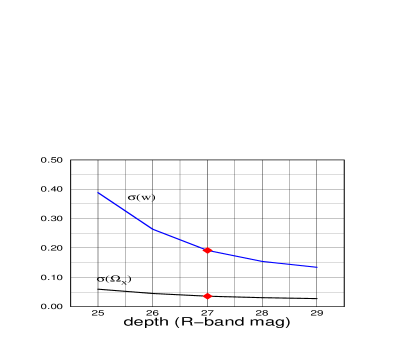
Figure 7: Dependence of $\sigma(\Omega_{X})$ and $\sigma(w)$ on the survey parameters. In each case we assume Planck (T) priors on other cosmological parameters. Diamonds denote the fiducial values. Top panel: 1-$\sigma$ uncertainties on $\Omega_{X}$ and $w$ as a function of sky coverage of the survey. We assume a fixed depth of 27th magnitude in $R$-band. Bottom panel: 1-$\sigma$ uncertainties on $\Omega_{X}$ and $w$ as a function of depth of the survey, assuming a fixed sky coverage of 1000 sq. deg.

V.6 Power spectrum Tomography

One way to extract more information out of the data would be to divide the lensed galaxies in several redshift bins and measure the convergence power spectrum in each bin, as well as the cross power spectrum between bins. This procedure, the power spectrum tomography, should be fully feasible with upcoming surveys because redshifts of source galaxies are going to be known quite accurately through photometric techniques.

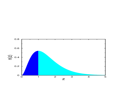
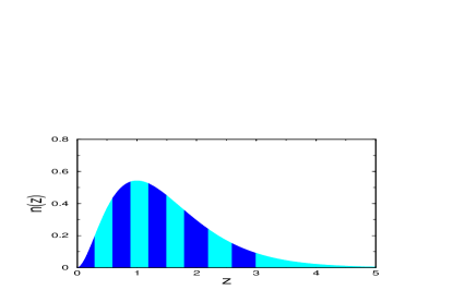
Figure 8: The divisions of source galaxies in redshift we used in order to implement the tomography. Top panel: A simple division in two redshift bins. Bottom panel: A division in 10 redshift bins.

Following the formalism of Hu tomography , we compute the parameter constraints when source galaxies are separated in redshift. Of the several slicings in two bins we tried, the most effective division was below and above $z=1.0$ (Fig. 8, top panel). In this case, the constraints on $\Omega_{X}$ and $w$ improve by a factor of 3 and 1.4 respectively, for a Planck(T) prior (Fig. 9). For the weaker COBE+photo-z prior, the improvement is even more significant: a factor of 5 and 3 improvements on $\Omega_{X}$ and $w$ respectively.

We also consider an optimistic scenario where galaxies can be separated in 10 redshift bins (Fig. 8, bottom panel). Whether or not and how accurately something like this can be done using photometric redshift techniques is presently under investigation (Eisenstein, Hu and Huterer, in preparation). The constraints on $\Omega_{M}$ (or $\Omega_{X}$) and $w$ further improve: $\sigma(\Omega_{X})=0.012$ and $\sigma(w)=0.07$ (Fig. 9).

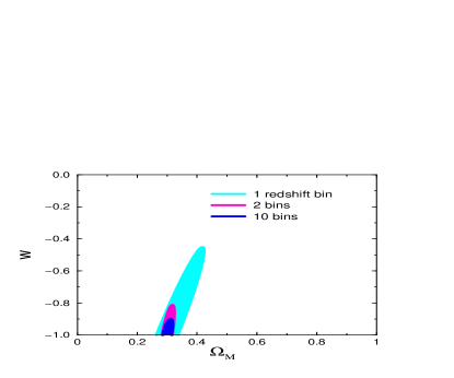
Figure 9: The improvement in the constraint on $\Omega_{M}$ and $w$ due to tomography. The 68% C.Ł. constraint regions correspond to 1, 2 and 10 divisions in redshift (largest to smallest ellipse), and are all computed using the Planck (T) prior.

Subdividing the galaxy population in more than two redshift bins leads to fairly limited improvements in parameter determination; this is due to high correlations ($\sim$80%) between the power spectra in different bins tomography . Nevertheless, tomography clearly adds valuable information on cosmological parameters and should be pursued with data from future WL experiments. In order to accurately assess and optimize this technique, further study considering realistic accuracy of photometric redshifts is necessary. Using simplified assumptions (in particular, no “leakage” of galaxies between bins), we have shown here that separation of galaxies in redshift easily leads to a factor of a few improvement in measuring $\Omega_{X}$ and $w$.

We now discuss whether a specific signature of certain dark-energy models can be detected with WL surveys.

V.7 Detecting the Dark-Energy Clustering?

Evolving scalar fields, or quintessence, are a particular class of candidates for dark energy (e.g. Wetterich ; Coble ; Zlatev ). One signature of quintessence is that it generally clusters around and above the Hubble radius scale $H_{0}^{-1}$. We ask: is it possible to detect this clustering in wide-field weak lensing surveys?

The clustering of quintessence is reflected in the increase in the transfer function on very large scales. The effect is more pronounced for larger $\Omega_{X}$ and larger $w$, and explicit forms for $T_{Q}(k,z)$ are given in Refs. Ma_QCDM and dark_synergy ; here $T_{Q}$ is the transfer function that takes clustering into account.

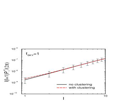
Figure 10: The effect of clustering of quintessence on the convergence power spectrum for a fiducial equation-of-state ratio $w=-1/3$. The error bars correspond to the cosmic variance for a full-sky weak lensing survey. Clustering affects the $l=1$ multipole the most, but even there the effect is buried within cosmic variance.

Clustering changes the matter power spectrum on large scales, which in turn alters the convergence power spectrum at lowest multipoles. In Figure 10 we show an optimistic scenario with $w=-1/3$ with and without clustering taken into account. We used exact formulae for the convergence power spectrum CMB_lens , since Limber’s approximation breaks down at lowest multipoles. Even though the effect on the matter power spectrum is significant ($T_{Q}(k,z)/T_{\Lambda}(k,z)\approx 2.0$ at $k\sim H_{0}$ in this case), the convergence power spectrum changes noticeably only at $l=1$, and even there only by $\sim 30\%$. As this Figure shows, the effect is buried deeply in the cosmic variance even for a full-sky WL survey. Therefore, it is unlikely that WL alone can detect the clustering of quintessence. However, cross-correlation of WL and other methods (e.g. the CMB) may be more promising; see Refs. Kinkhabwala ; Peiris .

VI Systematics and biases

VI.1 Observational issues

It is difficult to overemphasize the importance of controlling the various systematic errors that generically creep into the WL observing process. These include shear recovery issues, anisotropic point-spread function, the quality of seeing, and instrumental noise (for a nice study of systematic effects, see Ref. sys_study ). There is also the effect of overlapping galaxies, which is expected to be especially pronounced in very deep surveys, but might be overcome using the photometric redshift information (M. Joffre, private communication). Finally, the observed galaxies might be intrinsically aligned due to coupling of their angular momenta or a similar mechanism (Crittenden ; Croft_Metzler ; Heavens and references therein); this has already been observed Pen ; Brown . These effects may masquerade as the signal itself, and make the extraction of ellipticity correlations very difficult. In our analysis, we have assumed that these problems will be resolved, and that the dominant uncertainty will be the cosmic variance on large scales and Poisson noise on small scales. In that sense, our results (for a given parameter space, set of priors, and fiducial survey strategy) may be optimistic. On the other hand, rapid advances in our understanding of weak lensing techniques, as well as the prospects of powerful future surveys, indicate that in a few years we can expect a much better understanding of the aforementioned problems.

VI.2 Dependence upon nonlinear power spectrum and galaxy distribution

In addition to observational systematics that need to be controlled, theoretical prediction for the angular power spectrum of the convergence is also uncertain. Uncertainties in the nonlinear matter power spectrum (NLPS) and in the redshift distribution of galaxies are especially significant, as they are difficult to quantify and were not included in our analysis. We now discuss these two ingredients in more detail.

As can be seen from Figs. 2 and 4, most of our constraints come from nonlinear scales. Therefore, knowledge of the NLPS is crucial in order to compare experimental results with theory. However, this quantity is perhaps the most uncertain ingredient in the prediction for the power spectrum of the convergence. The NLPS is traditionally obtained by running N-body simulations for several cosmological models and deriving a fitting function to the simulated nonlinear power spectra. For the models with dark energy we consider, either PD or Ma QCDM fitting functions can be used. The latter was calibrated for quintessence models in a flat universe, and tested at $w=-2/3$, $-1/2$ and $-1/3$ and $\Omega_{M}=0.4$ and $0.6$.

Even with this solution, the intrinsic uncertainty of 5-15% in the NLPS is significant (recall, the transfer and growth functions are accurate to just a few percent). To illustrate the importance of knowing the NLPS accurately, let us for the moment assume that the true NLPS at $w=-1$ is that given by the formula of PD. Let us further assume that, not knowing this, we adopt the Ma QCDM prescription to compute the theoretical power spectra. We now compute the bias in cosmological parameters due to this “erroneous” assumption. Let us write the cosmological parameter values as

$$p_{i}=\bar{p}_{i}+\delta p_{i}$$ (31)

where $\bar{p}_{i}$ is the true value, $p_{i}$ the measured value, and $\delta p_{i}$ the bias due to using the “wrong” NLPS. Assuming that these biases are small, it is easy to show that Knox

$$\delta p_{i}=F_{ij}^{-1}\sum_{l}{1\over(\Delta P_{l}^{\kappa})^{2}}(P_{l}^{\kappa}-\bar{P}_{l}^{\kappa}){\partial\bar{P}_{l}^{\kappa}\over\partial p_{j}}$$ (32)

where $F_{ij}$ is the ubiquitous Fisher matrix, $P_{l}^{\kappa}$ ($\bar{P}_{l}^{\kappa}$) is the “erroneous” (“true”) power spectrum, and sum over $j$ is implied. The results of this exercise are given in Table 2 where we consider our fiducial survey with Planck (T) prior. The biases in $\Omega_{X}$ and $w$ are 2.5 and 4.8 times the 1-$\sigma$ uncertainties in these parameters! Even though these numbers may not be accurate because the approximation $\delta p\ll\bar{p}$ necessary to use Eq. (32) obviously did not hold, one can still conclude that the biases are very significant. Therefore, we need a more accurate knowledge of the NLPS.

TABLE 2

Parameter Biases Due to “wrong” NLPS Due to “wrong” $n(z)$ $p_{i}$ $|{\rm bias}|$ $|{\rm bias}|/\sigma(p_{i})$ $|{\rm bias}|$ $|{\rm bias}|/\sigma(p_{i})$ $\Omega_{X}$ $0.09$ $2.5$ $0.04$ $1.2$ $w$ $0.92$ $4.8$ $0.57$ $3.0$

Fortunately, the NLPS obstacle is surmountable. It is a matter of running powerful N-body simulations that include dark energy, on a fine grid in $w$ (and $m_{\nu}$ and other parameters, if necessary). Because we are only interested in the matter power spectrum (not galaxy power spectrum, which includes bias), N-body simulations can in principle give the NLPS to a very high accuracy. Once this is achieved, weak lensing will regain much of its power to probe dark energy.

Another quantity that may not be known to an extremely high accuracy (although we assumed so) is the redshift distribution of source galaxies $n(z)$. Indeed, current photometric redshift techniques can determine redshifts to an accuracy of $\sim 0.1$, depending on the redshift (e.g., Hogg ), which leaves room for error, both statistical and systematic. To include the uncertainty in $n(z)$, some authors (e.g., Jain_Seljak ; Bernardeau ; Hu_Tegmark ) parameterized the redshift distribution by one parameter only. However, the realistic uncertainty in $n(z)$ is much more difficult to quantify. To assess the effect of an uncertainty in the redshift distribution, we assume that the true distribution is given by Eq. (9) with $z_{0}=0.5$, while we “erroneously” assume the same form with $z_{0}=0.55$ (recall, $n(z)$ peaks at $z=2z_{0}$). The biases in $\Omega_{X}$ and $w$ are given in Table 2, and are 1.2 and 3.0 times the unbiased 1-$\sigma$ uncertainties in these parameters, respectively. Just as in the case of the NLPS, we conclude that accurate knowledge of the redshift distribution of galaxies will be crucial if weak lensing is to achieve its full potential.

VI.3 Power spectrum covariance

Yet another important issue that we ignored so far is covariance of the convergence power spectrum. The shear (or convergence) field is expected to be non-Gaussian due to nonlinear gravitational processes. Therefore, measurements of $P_{l}^{\kappa}$ are generally going to be correlated, implying a non-zero four-point function (or its Fourier analogue, the trispectrum). The covariance will be especially pronounced at high multipoles. For a survey down to a limiting magnitude of $R\sim 25$, the effect of power spectrum covariance appears to be small: Cooray & Hu Hu_covar have used the dark-matter halo approach to compute the power spectrum as well as the trispectrum, and found that the non-Gaussianity increases errors on cosmological parameters by about 15%. Although this effect is small enough to be ignored with current datasets, it will be important to take it into account when interpreting results from upcoming deep surveys because the covariance on small scales is likely to significantly degrade the cosmological constraints. Restricting our analysis (with COBE+photo-z prior) to multipoles $l\leq 3000$ degrades the constraints on $\Omega_{X}$ and $w$ by a factor of 5. Clearly, information from small scales is important, and it will be necessary to carefully assess the impact of power spectrum covariance for deep WL surveys.

VII Three-point statistics and dark energy

We now turn to three-point statistics of the weak lensing convergence. Unlike the CMB temperature fluctuations which may or may not be Gaussian, weak lensing convergence almost certainly does not obey Gaussian statistics. In this Section, we illustrate the dependence of the bispectrum and skewness of the convergence on dark energy, and show that they present a promising avenue that can lead to the dark component.

VII.1 Preliminaries

The bispectrum of the convergence $B_{l_{1}l_{2}l_{3}}^{\kappa}$ is defined through the three-point correlation function of the convergence in multipole space

$$\left<\kappa_{l_{1}m_{1}}\kappa_{l_{2}m_{2}}\kappa_{l_{3}m_{3}}\right>=\left(\begin{array}[]{ccc}l_{1}&l_{2}&l_{3}\\ m_{1}&m_{2}&m_{3}\end{array}\right)B_{l_{1}l_{2}l_{3}}^{\kappa}\,$$ (33)

and can further be written as

$$B_{l_{1}l_{2}l_{3}}^{\kappa} = \sqrt{(2l_{1}+1)(2l_{2}+1)(2l_{3}+1)\over 4\pi}\left(\begin{array}[]{ccc}l_{1}&l_{2}&l_{3}\\ 0&0&0\end{array}\right)$$ (36)

$$\times \left[\int d\chi{[W(\chi)]^{3}\over r(\chi)^{4}}B\left({l_{1}\over r(\chi)},{l_{2}\over r(\chi)},{l_{3}\over r(\chi)},\chi\right)\right]\,$$ (37)

The bispectrum is defined only if the following relations are satisfied: $|l_{j}-l_{k}|\leq l_{i}\leq|l_{j}+l_{k}|$ for $\{i,j,k\}\in\{1,2,3\}$ and $l_{1}+l_{2}+l_{3}$ is even. The term in parentheses is the Wigner 3j symbol, which is closely related to Clebsch-Gordan coefficients from quantum mechanics (for its properties, see Refs. Varshalovich ; Hu_reion ). $W(\chi)$ is the weight function defined in Sec. II. To compute the bispectrum of the convergence, therefore, we need to supply the matter bispectrum $B(k_{1},k_{2},k_{3},z)$. The latter quantity can be calculated in linear theory (that is, on large scales), but, just as in the case of the matter power spectrum, it needs to be calibrated from N-body simulations on nonlinear scales. Here we adopt the fitting formulae of Scoccimarro & Couchman (SC ; heretofore SC) which are based on numerical simulations due to VIRGO collaboration VIRGO . The matter bispectrum is defined only for closed-triangle configurations ($\vec{k}_{1}+\vec{k}_{2}+\vec{k}_{3}=0$) and is given by

$$B(\vec{k}_{1},\vec{k}_{2},\vec{k}_{3})=2\,F_{2}(\vec{k}_{1},\vec{k}_{2})P(k_{1})P(k_{2})+{\rm cycl.}$$ (38)

where $P(k)$ is the matter power spectrum and

$$F_{2}(\vec{k}_{1},\vec{k}_{2}) = {5\over 7}a(n,k_{1})\,a(n,k_{2})+$$ (39)

$${1\over 2}{\vec{k}_{1}\cdot\vec{k}_{2}\over k_{1}\,k_{2}}\left({k_{1}\over k_{2}}+{k_{2}\over k_{1}}\right)b(n,k_{1})\,b(n,k_{2})+$$

$${2\over 7}\left({\vec{k}_{1}\cdot\vec{k}_{2}\over k_{1}\,k_{2}}\right)^{2}c(n,k_{1})\,c(n,k_{2})$$

$n\equiv d\ln P/d\ln k$, and functions $a$, $b$ and $c$ are given in SC. Although not explicitly tested on models involving dark energy, the fitting formula depends on cosmology only through the matter power spectrum; this weak dependence on cosmology is also borne out in high-order perturbation theory SCFFHM . Therefore, we decide to use the SC formula to illustrate the dependence of three-point statistics on dark energy.

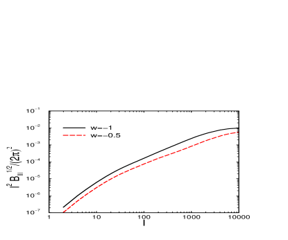
Figure 11: The quantity $l^{2}B^{1/2}_{lll}/(2\pi)$, involving equilateral-triangle configurations of the bispectrum in multipole space. We use this quantity to illustrate how the bispectrum depends on dark energy. The variance in $B_{lll}$ is roughly two orders of magnitude larger than the signal.

In Fig. 11 we show the quantity $l^{2}\sqrt{B_{lll}^{\kappa}}/(2\pi)$ Hu_bispec for $w=-1$ and $w=-0.5$; here $B_{lll}^{\kappa}$ is the equilateral triangle configuration of the bispectrum . Since roughly $B\propto P^{2}$ and $B$ has little other dependence on dark energy, we expect that $l^{2}\sqrt{B_{lll}^{\kappa}}/(2\pi)$ varies with $w$ similarly as $P$ — and this is correct (compare Figs. 2 and 11). Therefore, the bispectrum appears to be an excellent probe of dark energy. Things are complicated, however, by the large cosmic variance of a bispectrum. Although computing variance of $B$ involves a daunting task of evaluating the six-point correlation function of the convergence, this quantity can be computed under an assumption of small departures from Gaussianity Luo ; Gangui_Martin . For the equilateral triangle configuration of the bispectrum we show, this estimate indicates that the cosmic variance is about two orders of magnitude larger than the bispectrum signal itself, roughly independently of $l$. Therefore, it is unlikely that a single configuration of the bispectrum can be used to probe dark energy. However, one should be able to find an optimal combination of configurations in order to maximize the amount of information. We relegate this problem to future work.

Next we discuss the dependence of skewness on dark energy. Skewness is defined as

$$S_{3}(\theta)=\frac{\left<\kappa^{3}(\theta)\right>}{\left<\kappa^{2}(\theta)\right>^{2}}\,$$ (40)

where

$$\left<\kappa^{2}(\theta)\right> = {1\over 4\pi}\sum_{l}(2l+1)P_{l}^{\kappa}{\cal W}_{l}^{2}(\theta)$$ (41)

$$\left<\kappa^{3}(\theta)\right> = {1\over 4\pi}\sum_{l_{1}l_{2}l_{3}}\sqrt{(2l_{1}+1)(2l_{2}+1)(2l_{3}+1)\over 4\pi}$$ (44)

$$\times\left(\begin{array}[]{ccc}l_{1}&l_{2}&l_{3}\\ 0&0&0\end{array}\right)B_{l_{1}l_{2}l_{3}}^{\kappa}{\cal W}_{l_{1}}(\theta){\cal W}_{l_{2}}(\theta){\cal W}_{l_{3}}(\theta)\,.$$

are the second and third moments of the map smoothed over some angle theta, and ${\cal W}_{l}(\theta)$ is the Fourier transform of the top-hat function: ${\cal W}_{l}(\theta)=2J_{1}(l\theta)/(l\theta)$. Skewness effectively combines many different bispectrum configurations, and its variance should be much smaller than that of $B_{l_{1}l_{2}l_{3}}$. Its disadvantage is that measurements on different scales are correlated.

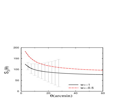
Figure 12: Skewness of the convergence for two values of $w$. Error bars are from simulations by White & Hu White_Hu on scales they explore and for a field of 36 sq. deg.

Fig. 12 shows skewness for two values of $w$. Roughly speaking, $S_{3}\propto B^{\kappa}/P^{2}$, and although $B^{\kappa}$ and $P^{2}$ both decrease with increasing $w$, the $P^{2}$ term prevails — hence the scaling of $S_{3}$ with $w$. The error bars shown are those from White & Hu White_Hu for their WL simulations corresponding to the $\Lambda$CDM model, and for a field of 36 sq. deg. Although the dependence of skewness on dark energy is significant, there are several obstacles. As in the case of the matter power spectrum, the fitting formula for the bispectrum is accurate only to about 15% (rms deviation) for $\Lambda$CDM models and not yet calibrated for dark energy models. More seriously, the measurements of skewness are likely to be highly correlated — in fact, van Waerbeke et al. vW_Scocc find that correlation between skewness measurements (for the top-hat filter we use) is close to 100%.

In conclusion, our preliminary analysis indicates that the three-point statistics of the weak lensing convergence are sensitive to the presence of dark energy, mainly through the dependence of the matter power spectrum. More work is needed, however, in order for the three-point statistic to become an effective probe of the missing component. This will include sharpening the predictions for the three-point function in the nonlinear regime, and finding optimal configurations of the bispectrum to probe dark energy.

VIII Discussion and Conclusions

Recent results coming from type Ia supernovae, CMB, and large-scale structure surveys make a strong case for the existence of dark energy. It is therefore important to explore how upcoming and future surveys can be used to probe this component. In this work, we explore the power of weak gravitational lensing to probe dark energy via its measurements of the power spectrum of the convergence.

Dark energy modifies the convergence power spectrum by altering the distance-redshift relation, as well as the matter power spectrum. The dependence on dark energy is therefore somewhat indirect, and cannot be easily disentangled from the effect of other parameters ($\Omega_{M}h^{2}$, $\Omega_{B}h^{2}$, $n$, $m_{\nu}$). Because of this, one would not expect WL to be an efficient way to probe dark energy. Nevertheless, we find that with the proposed very wide and deep surveys, WL can be an important probe of dark energy, on a par with SNe Ia and number counts. We consider a generic future survey covering 1000 sq. deg. down to a limited magnitude of $R=27$, cosmic-variance limited on large scales and Poisson-noise limited on small scales. With photometric redshift information and constraints on other parameters that would be expected from the Planck experiment with temperature information only, we find that such a survey is able to constrain $\Omega_{X}$ and $w$ to between a few percent and a few tens of percent, depending on the fiducial model and a chosen set of priors. The constraints are in general stronger for wider and deeper surveys, and depend on the fiducial model (e.g., the neutrino mass). Accurate knowledge of the redshift distribution of source galaxies will be crucial; we find that an error of only $0.05$ in the peak of the redshift distribution can bias the results.

There are important caveats to this result, however. Most information from WL comes from nonlinear scales, where the evolution of density perturbations is difficult to track analytically and understood mostly through N-body simulations (restricting the analysis of $P_{l}^{\kappa}$ only to linear scales with $l\lesssim 100$ would lead to extremely weak constraints on cosmological parameters due to cosmic variance). The nonlinearities potentially lead to at least two sources of systematic error. First, the power spectrum measurements $P_{l}^{\kappa}$ are likely to be strongly correlated at multipoles of several thousand and higher. This is especially true for planned deep surveys (down to a limited magnitude of $R\sim 27$ or higher), and these correlations will likely degrade the constraints on $\Omega_{X}$ and $w$.

Second, although the nonlinear power spectrum has been calibrated quite accurately for $\Lambda$CDM models, most notably through the PD formula, it remains poorly explored for models with general equation of state $w$, massive neutrinos, and significant baryon density. We explicitly showed that the lack of knowledge of the dependence of the nonlinear power spectrum on $w$ can easily bias the constraints on $\Omega_{X}$ and $w$. Therefore, a better understanding and calibration of the NLPS is absolutely crucial in order to use WL as a tool of precision cosmology.

This problem can be turned around, however. One could use the weak lensing measurements (combined, perhaps, with information from CMB measurements, SNe Ia, and other probes) in order to constrain the nonlinear power spectrum. This constraint could be very interesting, given the strong dependence of the NLPS on cosmological parameters.

Predictions for the three-point statistics of WL are quite uncertain at present, especially for models involving dark energy. This does not mean they will not become effective probes of the missing component in the future. We estimate the equilateral bispectrum configuration, as well as skewness, for two values of $w$ and show that dependence on $w$ is significant. Although these two quantities are plagued by large cosmic variance and highly correlated noise respectively, by clever choice of bispectrum configurations one might be able to increase the signal-to-noise ratio and extract useful information on dark energy.

There are other ways to use weak lensing as a probe of cosmology which we did not discuss. For example, one could use WL to identify clusters of galaxies at redshifts $0<z\lesssim 3$ (M. Joffre et al., in preparation). Comparing the measured number density of clusters to the prediction given by the formalism of Press & Schechter PS gives constraints on cosmology. Another idea is to measure the angular power spectrum of clusters (detected through WL) at different redshifts cluster_PS ; this gives a direct measure of the angular diameter distance as a function of redshift. The advantage of this approach is that only the linear matter power spectrum is required; furthermore, the mass function and profiles of clusters need not be known. These two methods will provide constraints complementary to those from the galaxy shear.

Weak gravitational lensing is likely to provide a wealth of information not only on the matter distribution in the universe, but also on the amount and nature of dark energy. We have considered the basic program of measuring the convergence power spectrum, and found that very wide and deep surveys could provide information complementary and comparable to that from other cosmological probes. Other statistics (various bispectrum configurations, cross-correlation of WL and the CMB, etc.) are likely to further increase the power of weak lensing and make it an important probe of dark energy.

- (1) A. Riess et al., Astron. J., 116, 1009 (1998)
- (2) S. Perlmutter et al., Astrophys. J. 517, 565 (1999)
- (3) D. Huterer and M. S. Turner, Phys. Rev. D 60, 081301 (1999)
- (4) J. Weller and A. Albrecht, report DAMTP-2001-53 (astro-ph/0106079)
- (5) I. Maor, R. Brustein, and P. J. Steinhardt, Phys. Rev. Lett. 86, 6 (2001)
- (6) M. Goliath, R. Amanullah, P. Astier, A. Goobar, A. and R. Pain, astro-ph/0104009
- (7) M. S. Turner, Physica Scripta T85, 210 (2000)
- (8) D. Huterer and M. S. Turner, Phys. Rev. D in press (astro-ph/0012510)
- (9) Z. Haiman, J. J. Mohr, and G. P. Holder, Astrophys. J. 553, 545 (2001)
- (10) J. Newman and M. Davis, Astrophys J. 534 , L11 (2000)
- (11) J. A. Tyson, F. Valdes, J. F. Jarvis and A. P. Jr. Mills, Astrophys. J., 281, L59 (1984)
- (12) J. Miralda Escudé, Astrophys. J., 380, 1 (1991)
- (13) R. Blanford, A. Saust, T. Brainerd and J. Villumsen, Mon. Not. R. Astron. Soc., 251, 600 (1991)
- (14) N. Kaiser, Astrophys. J., 388, 272 (1992)
- (15) N. Kaiser, Astrophys. J., 498, 26 (1998)
- (16) B. Jain and U. Seljak, Astrophys. J., 484, 560 (1997)
- (17) M. Kamionkowski, A. Babul, C. M. Cress, and A. Refregier, Mon. Not. R. Astron. Soc., 301, 1064 (1998)
- (18) N. Kaiser and G. Squires, Astrophys. J., 404, 441 (1993)
- (19) Y. Mellier, Proceedings of the NATO Advanced Study Institute on Theoretical and Observational Cosmology, ed. Marc Lachieze-Rey; Kluwer Academic, 1999.; astro-ph/9901116
- (20) D. Wittman, J. A. Tyson, D. Kirkman, I. Dell’Antonio and G. Bernstein, Nature, 405, 143 (2000)
- (21) D. J. Bacon, A. R. Refregier and R. S. Ellis, Mon. Not. R. Astron. Soc., 318, 625 (2000)
- (22) L. Van Waerbeke et al., A&A 358, 30 (2000)
- (23) N. Kaiser, G. Wilson and G. A. Luppino, astro-ph/0003338
- (24) M. S. Turner and M. White, Phys. Rev. D, 56, R4439 (1997)
- (25) F. Bernardeau, L. Van Waerbeke and Y. Mellier, A&A, 322, 1 (1997)
- (26) W. Hu and M. Tegmark, Astrophys. J., 514, L65 (1999)
- (27) C. B. Netterfield et al. astro-ph/0104460
- (28) C. Pryke et al., astro-ph/0104490
- (29) R. Stompor et al., astro-ph/0105062
- (30) X. Wang, M. Tegmark and M. Zaldarriaga, astro-ph/0105091
- (31) M. Bartelmann and P. Schneider, Physics Reports, 340, 291 (2001)
- (32) W. Hu and M. White, Astrophys. J., 519, L9 (2000)
- (33) T. Broadhurst, astro-ph/9505010
- (34) C. L. Bennett et al., Astrophys. J., 464, L1 (1996)
- (35) C.-P. Ma, R. R. Caldwell, P. Bode and L. Wang, Astrophys. J., 521, L1 (1999) (Ma QCDM)
- (36) E. F. Bunn and M. White, Astrophys. J., 480, 6 (1997)
- (37) A. Liddle and D. Lyth, ”Cosmological inflation and large-scale structure”, Cambridge University Press (2000)
- (38) W. Hu and D. J. Eisenstein, Astrophys. J., 498, 497 (1998)
- (39) S. M. Carroll, W. H. Press and E. L. Turner, ARA&A 30, 499 (1992)
- (40) P. J. E. Peebles, ”Principles of Physical Cosmology”, Princeton University Press (1993)
- (41) A. J. S. Hamilton, A. Matthews, P. Kumar and E. Lu, Astrophys. J., 374, L1 (1991)
- (42) J. A. Peacock and S. J. Dodds, Mon. Not. R. Astron. Soc., 267, 1020 (1994) (PD)
- (43) C.-P. Ma, Astrophys. J., 508, L5 (1998) (Ma LCDM)
- (44) M. Tegmark, A. N. Taylor, and A. F. Heavens, Astrophys. J. 480, 22 (1997)
- (45) M. Zaldarriaga and U. Seljak, Phys. Rev. D., 55, 1830 (1998)
- (46) D. Eisenstein, W. Hu, M. Tegmark, Astrophys. J. 518, 2 (1999)
- (47) M. Tegmark, D. J. Eisenstein, W. Hu and R. Kron, astro-ph/9805117
- (48) G. P. Holder, Z. Haiman and J. J. Mohr, ApJL, in press Astrophys. J., 560, L111 (2001)
- (49) N. Metcalfe, T. Shanks, A. Campos, H. J. McCracken and R. Fong, Mon. Not. R. Astron. Soc., 323, 795 (2001)
- (50) D. W. Hogg et al.,AJ, 115, 1418 (1998)
- (51) R. Croft, W. Hu and R. Davé, Phys. Rev. Lett., 83, 1092 (1999)
- (52) W. Hu, Astrophys. J., 522, L21 (1999)
- (53) C. Wetterich, Nucl. Phys. B 302, 668 (1988)
- (54) K. Coble, S. Dodelson, and J. Frieman, Phys. Rev. D 55, 1851 (1996)
- (55) I. Zlatev, L. Wang and P. J. Steinhardt, Phys. Rev. Lett. 82, 896 (1999)
- (56) W. Hu, Phys. Rev. D, submitted (astro-ph/0108090)
- (57) W. Hu, Phys. Rev. D, 62, 043007 (2000)
- (58) A. Kinkhabwala and M. Kamionkowski, Phys. Rev. Lett., 82, 4172 (1999)
- (59) H. V. Peiris and D. N. Spergel, 2000, Astrophys. J., 540, 605 (2000)
- (60) D. J. Bacon, A. Refregier, D. Clowe and R. S. Ellis, Mon. Not. R. Astron. Soc., 325, 1065 (2001)
- (61) R. G. Crittenden, P. Natarajan, U.-L. Pen and T. Theuns, Astrophys. J., 559, 552 (2001)
- (62) R. Croft and C. Metzler, Astrophys. J., 545, 561 (2000)
- (63) A. Heavens, A. Refregier and C. Heymans, Mon. Not. R. Astron. Soc., 319, 649 (2000)
- (64) U.-L. Pen, J. Lee and U. Seljak, Astrophys. J., 543, L107 (2000)
- (65) M. L. Brown, A. N. Taylor, N. C. Hambly and S. Dye, astro-ph/0009499
- (66) L. Knox, R. Scoccimarro and S. Dodelson, Phys. Rev. Lett., 81, 2004 (1998)
- (67) A. Cooray and W. Hu, Astrophys. J., 554, 56 (2001)
- (68) D. A. Varshalovich, A. N. Moskalev and V. K. Kheronskii, “Quantum THeory of Angular Momentum”, World Scientific (1998)
- (69) A. Cooray and W. Hu, Astrophys. J., 534, 533 (2000)
- (70) R. Scoccimarro and H. Couuchman, Mon. Not. R. Astron. Soc., 325, 1312 (2001)
- (71) A. R. Jenkins et al., Astrophys. J., 503, 37 (1998)
- (72) L. Van Waerbeke, T. Hamana, R. Scoccimarro, S. Colombi and F. Berardeau, Mon. Not. R. Astron. Soc., 322, 918 (2001)
- (73) A. Cooray and W. Hu, Astrophys. J., 548, 7 (2001)
- (74) R. Scoccimarro, S. Colombi, J. N. Fry, J. A. Frieman, E. Hivon and A. Melott, Astrophys. J., 496, 586 (1998)
- (75) X. Luo, Astrophys. J., 427 L71 (1994)
- (76) A. Gangui and J. Martin, Mon. Not. R. Astron. Soc., 313, 323 (2000)
- (77) M. White and W. Hu, Astrophys. J., 537, 1 (2000)
- (78) W. H. Press and P. L. Schechter, Astrophys. J., 187, 425 (1974)
- (79) A. Cooray, W. Hu, D. Huterer and M. Joffre, Astrophys. J., 557 L7 (2001)