Galaxy clustering in the Sloan Digital Sky Survey (SDSS): A first comparison with the APM Galaxy Survey

Abstract

We compare the large scale galaxy clustering in the new SDSS early data release (EDR) with the clustering in the APM Galaxy Survey. We cut out pixel maps (identical in size and shape) from the SDSS and APM data to allow a direct comparison of the clustering. Here we concentrate our analysis on an equatorial SDSS strip in the South Galactic Cap (EDR/SGC) with 166 $deg^{2}$, 2.5 wide and 65 degrees long. Only galaxies with Petrosian magnitudes $16.8<g^{\prime}<19.8$ are included to match the surface density of the $17<b_{J}<20$ APM pixel maps (median depth of $\sim 400\;h^{-1}{\rm Mpc}$). Both the amplitude and shape of the angular 2-point function and variance turn out to be in very good agreement with the APM on scales smaller than 2 degrees (or $\la 15\;h^{-1}{\rm Mpc}$). The 3-point function and skewness are also in excellent agreement within a $90\%$ confidence level. On one hand these results illustrate that the EDR data and SDSS software pipelines, work well and are suitable to do analysis of large scale clustering. On the other hand it confirms that large scale clustering analysis is becoming ”repeatable” and therefore that our conclusions for structure formation models seem to stand on solid scientific grounds.

1 Introduction

The Sloan Digital Sky Survey (SDSS) uses a dedicated 2.5 m telescope and a large format CCD camera to obtain images of over 10,000 $deg^{2}$ of high Galactic latitude sky in five broad bands. The SDSS represents a new paradigm of scientific project, where digital data is made available on-line to the community via ”virtual observatories”. On June 2001 the SDSS collaboration made an early data release (EDR) publicly available. In this paper, we take this opportunity to do a study of some large scale structure aspects of the EDR. We compare this new data with the APM Galaxy Survey (Maddox etal 1990), which is based on 185 UK IIIA-J Schmidt photographic plates each corresponding to $6\times 6$ square degrees on the sky limited to $b_{J}\simeq 20.5$ and covering $b<-40$ and $\delta<-20$ degrees. These fields where scanned by the APM machine and carefully matched using the plate overlaps.

The APM Survey has produced one of the best estimates of the angular galaxy 2-point correlation function $w_{2}(\theta)$ to date. Its shape on large scales led to the discovery of “extra” large-scale power, and gave early indications for the paradigm shift out of the standard (Einstein-de Sitter) CDM model (Maddox etal 1990). Frieman & Gaztañaga (1999, FG99 hereafter) estimated the 3-point galaxy correlation function in the APM Galaxy Survey and its comparison with theoretical expectations (see also Peebles 1980, Fry 1984, Juszkiewicz, Bouchet & Colombi 1993, Fry & Gaztañaga 1993, Gaztañaga 1994, Bernardeau 1994, Fosalba & Gaztañaga 1998, Buchalter, Jaffe & Kamionkowski 2000, Scoccimarro etal. 2001, and references therein). For the first time, the APM measurements extended to sufficiently large scales to probe the weakly non-linear regime with a reliable Survey. The results are in good agreement with gravitational growth for a model with initial Gaussian fluctuations. They also indicate that the APM galaxies are relatively unbiased tracers of the mass on large scales and provide stringent constraints upon models with non-Gaussian initial conditions.

Linear CCD devices provide more reliable magnitudes than the traditional non-linear system of visual magnitudes. Scanned plates should do better, but there has been extended discussions regarding variable sensitivity inside individual Schmidt plates and large-scale gradients in the APM survey calibration. A CCD survey, such as the SDSS, reduces these systematic effects and could provide more accurate photometry and luminosity function estimators (eg Blanton etal 2001, see also Gaztañaga & Dalton 2000). Thus, a natural question arrises: is the large scale clustering trace by the new SDSS digital data compatible with the one measured in the old photographic APM scans? As there is no spatial overlap between these two data sets, we will compare the statistical properties, such as correlation functions and moments of counts in cells. The answer to this question will bring new evidence to our understanding of structure formation in the lines mentioned above.

2 SDSS sample and pixel maps

We download data from the SDSS public archives using the SDSS Science Archive Query Tool (sdssQT, http://archive.stsci.edu/sdss/software/). We select objects from an equatorial SGC (South Galactic Cap) strip 2.5 wide ($-1.25<DEC<1.25$ degrees.) and 66 degrees long ($351<RA<56$ degrees.) which seems to be homogeneous. This strip (SDSS numbers 82N/82S) corresponds to some of the first runs of the early commissioning data (runs 94 and 125) with variable seeing conditions (a few tenths of arc-second within scales of a few degrees. ). To avoid confusion with the EDR equatorial strip in the North (studied by the SDSS collaboration, eg in Scranton et al 2001) we will refer to this strip as EDR/SGC.

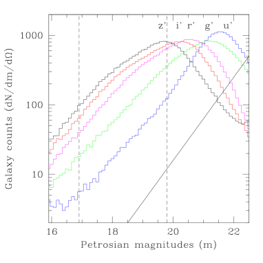
We first select all galaxies brighter than $u^{\prime}=22.3,g^{\prime}=23.3,r^{\prime}=23.1,i^{\prime}=22.3,z^{\prime}=20.8$, which corresponds to the SDSS limiting magnitudes for 5 sigma detection in point sources (York etal. 2000). Galaxies are found from either the $1\times 1$, $2\times 2$ or $4\times 4$ binned CCD pixels and they are deblended by the SDSS pipeline (Lupton etal 2001). There are about 375000 objects classified as galaxies in the EDR/SGC. Figure 1 shows the number counts (surface density) for these 375000 galaxies as a function of the magnitude in each band, measured by the SDSS modified Petrosian magnitudes $m_{u}^{\prime}$, $m_{g}^{\prime}$, $m_{r}^{\prime}$, $m_{i}^{\prime}$ and $m_{z}^{\prime}$ (see Yasuda et al 2001 for a discussion of the SDSS counts). Continuous diagonal lines show the $10^{0.6m}$ expected for a low redshift homogeneous distribution with no k-correction, no evolution and no-extinction. The limiting magnitudes for detecting galaxies in this strip seems to be closer to $m_{u}^{\prime}<21.5$, $m_{g}^{\prime}<21$, $m_{r}^{\prime}<20.5$, $m_{i}^{\prime}<20$ and $m_{z}^{\prime}<19.5$.

We next select galaxies with SDSS modified Petrosian magnitudes $16.8<m_{g}^{\prime}<19.8$. We choose $g^{\prime}$ because this is the closest SDSS band to the APM blue $b_{J}$. The range $16.8<m_{g}^{\prime}<19.8$ results from requiring that the SDSS surface density in a 3 magnitude slice equals that of the APM in the $17<b_{J}<20$ slice (ie $\simeq 300$ gal per $deg^{2}$). We have checked that small departures from this range produce similar clustering results. There are about 54000 galaxies that match this criteria in the EDR/SGC. Figure 1 shows that the number counts in this range of magnitudes (limit by the two dashed vertical lines in the figure) follow well the $10^{0.6m}$ relation (continuous line), indicating that the sample selected is homogeneous and completed to this magnitude. We do not apply any mask to the EDR/SGC sample or try to make any correction for variable seeing or variable extinction across the strip. Visually, there are no obvious holes or inhomogeneities in the pixel maps at this depth. We will assume that variations in extinction and seeing do not affect clustering of the relatively bright galaxies we are considering (see a detailed study by Scranton etal 2001).

Figure 1: Galaxy density counts per magnitude and square deg. $dN/dm/d\Omega$ as a function of Petrosian magnitude $z^{\prime},i^{\prime},r^{\prime},g^{\prime},u^{\prime}$ (from left to right).

Figure 2: Pixel maps showing number density of galaxies increasing from 0 (black) to about 15 (white) galaxies per cells of $7$ arc-min. The equatorial strip of $66$ degrees in RA and 2.5 degrees wide is cut in 4 overlapping pieces to fit the page.

Finally, we produce equal area projection pixel maps of various resolutions , similar to those made for the APM (see Plate 1 in Maddox etal 1990). Figure 2 shows the EDR/SGC pixel maps with a resolution of about $7$ arc-min. It is apparent that there are important surface density variations along the strip, even on the largest scales. One can also see filamentary structure and a overall texture similar to that in the APM pixel maps (see Plate 1 in Maddox etal. 1990) or the Lick maps (see cover of Peebles 1993).

3 Clustering comparison

Our goal is to compare the APM to the new SDSS data. Out of the APM Survey we considered a $17<b_{J}<20$ magnitude slice in an equal-area projection pixel map with a resolution of $3.5$ arc-min, that covers over $4300$ $deg^{2}$ around the SGC. The APM can fit over 25 strips of similar area, shape and depth as the SDSS strip shown in Figure 1. To study sampling and biasing effects on the SDSS clustering estimators (due to the limited survey area), we have cut 10 strips out of the APM map. Each of these 10 sub-samples are identical in size and shape to the EDR/SGC SDSS strip, and are separated from each other by few degrees, so that they can be considered as independent. This will allow us to set $\simeq 90\%$ confidence intervals against the null hypothesis that the EDR/SGC strip is compatible with the APM map. In all cases we correct the clustering in the APM maps for a $5\%$ contamination of randomly merged stars (see Maddox etal 1990), ie we scale fluctuations up by $5\%$ (see also Gaztañaga 1994).

3.1 Smoothed 1-point Moments

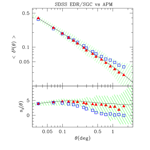
We first compare the lower order moments of counts in cells of variable size $\theta$ (larger than the pixel map resolution). We follow closely the corresponding APM analysis in Gaztañaga (1994, see also Szapudi etal 1995) and use the same software and estimators here for the SDSS. The top panel in Fig. 3 shows the variance of fluctuations in density counts $\delta\equiv\rho/{\bar{\rho}}-1$ smoothed over a scale $\theta$: $\bar{w_{2}}\equiv<\delta^{2}(\theta)>$, which is plotted as a function of the smoothing radius $\theta$. The shaded region shows the $\simeq 90\%$ confidence interval for the SDSS results to be compatible to the APM map. This shaded region brackets the minimum and maximum results at each scale in the 10 APM sub-samples that mimic the EDR/SGC. The individual results in each subsample are strongly correlated so that the whole curve for each subsample scales up an down inside the shaded region, ie there is a strong covariance at all separations due to large scale density fluctuations. Triangles correspond to the mean of the 10 APM sub-samples, which are slightly bias down as compared to the whole APM (continuous line). The SDSS results (open squares) are all within the $90\%$ confidence region set by the APM. Because of the strong covariance mentioned above, we do not expect the SDSS values to scatter around the APM values, but rather we expect the whole curved to be shifted, as shown in the Figure. This is also the case for the other statistical measures presented below.

The extend of the shaded area would narrow if we increase the total solid angle of the subsamples. Numerical simulations show that the corresponding error-bar is about a factor of 4-6 smaller for a survey as large as the APM.

Figure 3: The variance $\bar{w_{2}}$ (top panel) and reduced skewness (bottom panel) as a function of angular smoothing $\theta$. Squares correspond to the SDSS EDR/SGC strip. The triangles and the shaded area correspond to the mean and $90\%$ confidence level in the values of 10 APM sub-samples with same size and shape as the SDSS. The continuous line corresponds to the whole APM map.

The bottom panel in Fig. 3 shows the corresponding comparison for the normalized angular skewness:

$$s_{3}(\theta)\equiv{<\delta^{3}(\theta)>\over{<\delta^{2}(\theta)>^{2}}}\equiv{\bar{w_{2}}(\theta)\over{\bar{w_{3}}(\theta)}}$$ (1)

Again the mean of the individual APM zones (triangles) does not equal the whole APM estimation (continuous line). This is due to estimation (or ratio) bias (see Hui & Gaztañaga 1999). The SDSS EDR/SGC data on $s_{3}$ shows an excellent agreement with the APM at the smaller scales (in contrast with the EDSGC results, see Szapudi & Gaztañaga 1998). On larger scales the SDSS values are smaller, but the discrepancy is not significant within the $90\%$ region and given the strong covariance of individual subsamples. Similar results are found for higher order moments. As we approach the scale of $2$ degrees, the width of our strip, it becomes impossible to do counts for larger cells. It is therefore interesting to study the correlation functions, which should be less affected by boundary effects (although sampling effects will still be important).

3.2 N-point Correlation functions

We next study the angular 2-point, $w_{2}\equiv<\delta_{1}\delta_{2}>$, and 3-point, $w_{3}\equiv<\delta_{1}\delta_{2}\delta_{3}>$, correlation functions. Here we follow closely the notation, estimators and software used in FG99. The 3-point function is normalized as:

$$q_{3}\equiv{w_{3}(\theta_{12},\theta_{13},\theta_{23})\over w_{2}(\theta_{12})w_{2}(\theta_{13})+w_{2}(\theta_{12})w_{2}(\theta_{23})+w_{2}(\theta_{13})w_{2}(\theta_{23})}$$ (2)

where $\theta_{12}$, $\theta_{13}$ and $\theta_{23}$ correspond to the sides of the triangle form by the 3 angular positions of $\delta_{1}\delta_{2}\delta_{3}$. Here we will consider isosceles triangles, ie $\theta_{12}=\theta_{13}$, so that $q_{3}=q_{3}(\alpha)$ is given as a function of the interior angle $\alpha$ which determines the other side of the triangle $\theta_{23}$ (FG99). We also consider the particular case of the collapsed configuration $\theta_{23}=0$, which corresponds to $<\delta_{1}\delta_{2}^{2}>$ and is normalized in slightly different way (see also Szapudi & Szalay 1999):

$$c_{12}\equiv{<\delta_{1}\delta_{2}^{2}>\over{<\delta_{1}\delta_{2}><\delta_{1}^{2}>}}\simeq 2q_{3}(\alpha=0)~{}.$$ (3)

Figure 4: Same as Fig.3 for the 2-point function (top panel) and the collapsed 3-point function, $c_{12}$, as a function of scale $\theta$.

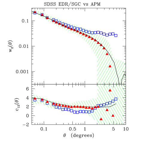
Top panel in Fig.4 shows the 2-point correlation as a function of the separation $\theta$ between points (here small pixel cells). Results from both surveys agree remarkably well up to 1 degree. In a similar way as to what happened with the variance (ie Fig.3) the SDSS EDR/SGC sample shows a flatting of the $w_{2}$ slope at large scales. At scales bigger than $\simeq 3$ degrees this discrepancy becomes significant and it is incompatible with the APM subsamples with a confidence level higher that $90\%$. This deviation could be due to systematic gradients in the SDSS raw data that we are using (eg due to large seeing variation across the strip, see §2 above). But it could also be due to an underestimation of the sampling errors in the APM (eg due to smoothing of the APM calibration on the scale of the subsamples). We need to consider larger and better calibrated areas to confirm or refute with the SDSS the features in APM galaxy power spectrum shape discussed in Gaztañaga & Baugh (1998, and references therein) and Gaztañaga & Juszkiewicz (2001). At smaller scales, the agreement is excellent and the measured shape of the SDSS 2-point function confirms the idea that galaxies are ’anti-bias’ with respect to the $\Lambda$CDM model (eg Gaztañaga 1995, Jenkins etal 1998, and references therein).

Figure 5: Same as Fig.3 for 3-point function $q_{3}(\alpha)$.

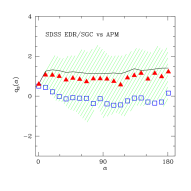
Bottom panel of Fig.4 and Fig.5 shows the reduced 3-point function $q_{3}$ for different configurations. Fig.5 compares $q_{3}(\alpha)$ for isosceles triangles of side $\theta_{12}=\theta_{13}=0.5$ degrees. Bottom panel of Fig.4 shows the collapsed case $c12\simeq 2q_{3}(\alpha=0)$ as a function of the other triangle side $theta=\theta_{12}=\theta_{13}$. The reduced 3-point function in Fig.5 is close to zero and the signal seems stronger on smaller scales. In all cases, the SDSS results are within the $90\%$ confidence of the APM values. Note again the bias between the mean of the 10 APM strips (triangles) and the whole APM (continuous line), and also the strong covariance across the curves. As mentioned above both of these results are expected and due to (very) large scale density fluctuations.

4 Discussion and conclusions

We have presented a rigorous $90\%$ confidence test for the hypothesis that the clustering in the SDSS EDR/SGC strip is compatible with the one in the APM data. The test is passed for clustering at scales smaller than 2 degrees (which corresponds to $\simeq 15Mpc/h$), and seems to fail (at $90\%$ confidence) at larger scales. This could be due to large scale variations in the seeing (on scales of a few degrees) present in the early SDSS commissioning data (EDR/SGC) that we are using (see §2), but they could also reflect the fact that the APM sampling errors are not accurate at this level. In principle, it is possible to correct for these seeing gradients by using the appropriate mask (see Scranton etal 2001), but we have not attempted to do this here.

The agreement between these two catalogues, on scales smaller than 2 degrees, is not trivial: correlation functions are quite sensitive to systematic effects and clustering for galaxies of fainter magnitudes or different colors is quite different. Moreover, we have not rescale or match the amplitudes of the two catalogues: the agreement comes naturally when we just select galaxies with the same colors, magnitude range and similar surface density in both samples. It is hard to belive that this is just a coincidence. These results rather illustrates that EDR data and software pipelines from SDSS work well and are suited to do analysis of large scale clustering.

We find it remarkable that two totally independent surveys, separated in space (ie angular position and spectral filtering) and time (over 10 years in technological and software development) provide very similar results for the large scale angular clusterings trace by galaxies. This is true both visually and by accurate statistical comparisons. It illustrates that large scale clustering analysis is becoming ”repeatable” and therefore that our conclusions could stand on solid scientific grounds. In particular, one conclusion that we have been able to confirm in this work, is that the higher order correlations in galaxy samples indicate that gravitational growth from Gaussian initial conditions is responsible for the hierarchical structures we see in the sky (eg FG99, Scoccimarro etal 2001, and references therein). When more of the SDSS data is analyzed we can hope to make much higher precession testing of our models for structure formation (eg Tegmark etal 1998; Colombi etal 2000).

References

- [1]
- [ref] Bernardeau, F., 1994, A&A 291, 697
- [2] Blanton, M.R. etal, 2001, A.J., 121, 2358
- [ref] Buchalter, A., Jaffe, A., Kamionkowski, M., 2000, ApJ, 530, 36
- [3] Colombi, S., Szapudi, I., Jenkins, A., Colberg, J., 2000, MNRAS313, 711
- [ref] Fosalba, P. & Gaztañaga, E., 1998, MNRAS301, 503
- [Frieman & Gaztañaga 1999] Frieman, J.A., Gaztañaga, E., 1999, ApJ, 521, L83 (FG99)
- [ref] Fry, J. N. 1984, ApJ, 279, 499
- [ref] Fry, J. N. & Gaztañaga, E. 1993, ApJ, 413, 447
- [Gaztañaga 1994] Gaztañaga, E., 1994, ApJ, 454, 561
- [Gaztañaga 1995] Gaztañaga, E., 1995, MNRAS, 268, 913
- [Gaztañaga 1998] Gaztañaga, E., & Baugh, C.M. 1998, MNRAS, 294, 229
- [Gaztañaga 2000] Gaztañaga, E. & Dalton, G.B., 2000, MNRAS, 312, 417
- [4] Gaztañaga, E. & R. Juszkiewicz, 2001, R. ApJ, 558, L1
- [5] Hui, L.& Gaztañaga, E., 1999, ApJ, 519, 622
- [6] Jenkins, A. etal 1998, ApJ499, 20
- [ref] Juszkiewicz, R., Bouchet, F., & Colombi, S. 1993, ApJ, 412, L9
- [ref] Lupton, R., Gunn, J.E., Ivezić, Z Knapp, G.R., Kent, S., Yasuda, N, 2001, in ASP Conf. Ser. 238, Astronomical Data Analysis Software and Systems X, ed. F.R. Harnden, F.A. Primini and H.E.Payne, in press astro-ph/0101420
- [7] Maddox, S.J., Efstathiou, G., Sutherland, W.J. & Loveday, J., 1990, MNRAS, 242, 43P
- [Peebles 1993] Peebles, P.J.E., 1993, Principles of Physical Cosmology, Princeton University Press, Princeton
- [Peebles 1993] Peebles, P.J.E., 1980, The Large Scale Structure of the Universe, Princeton: Princeton University Press
- [8] Scoccimarro, R., Feldman, H., Fry, J. N. & Frieman, J.A., 2001 ApJ, 546, 652
- [9] Scranton, R., Johnston, D., Dodelson, S. etal astro-ph/0105545, submitted to ApJ. 2001
- [10] Szapudi, I., Dalton, G.B. , Efstathiou, G. & Szalay, A.S., 1995, ApJ444, 520
- [11] Szapudi, I. & Gaztañaga, E., 1998, MNRAS300, 493
- [12] Szapudi, I., & Szalay, A.S., 1999, ApJ, 515 L43
- [13] Tegmark, M., Hamilton, A.J.S., Strauss, M.A., Vogeley, M.S. & Szalay, A.S. 1998, ApJ, 499, 555
- [14] Yasuda, N., Fukugita, M., Narayaran, V.K. etal 2001 astro-ph/0105545, submitted to ApJ.
- [15] York, D.G. etal, 2000, A.J., 120, 1579 astro-ph/0006396