The SCUBA Local Universe Galaxy Survey II. 450$\mu$m data – evidence for cold dust in bright IRAS Galaxies.

Abstract

This is the second in a series of papers presenting results from the SCUBA Local Universe Galaxy Survey. In our first paper we provided 850$\mu$m flux densities for 104 galaxies selected from the IRAS Bright Galaxy Sample and we found that the 60, 100$\mu$m (IRAS) and 850$\mu$m (SCUBA) fluxes could be adequately fitted by emission from dust at a single temperature. In this paper we present 450$\mu$m data for the galaxies. With the new data, the spectral energy distributions of the galaxies can no longer be fitted with an isothermal dust model – two temperature components are now required. Using our 450$\mu$m data and fluxes from the literature, we find that the 450$\mu$m/850$\mu$m flux ratio for the galaxies is remarkably constant and this holds from objects in which the star formation rate is similar to our own Galaxy, to ultraluminous infrared galaxies (ULIRGS) such as Arp 220. The only possible explanation for this is if the dust emissivity index for all of the galaxies is $\sim 2$ and the cold dust component has a similar temperature in all galaxies ($T_{c}\sim 20-21$ K). The 60$\mu$m luminosities of the galaxies were found to depend on both the dust mass and the relative amount of energy in the warm component, with a tendency for the temperature effects to dominate at the highest $L_{60}$. The dust masses estimated using the new temperatures are higher by a factor $\sim 2$ than those determined previously using a single temperature. This brings the gas-to-dust ratios of the IRAS galaxies into agreement with those of the Milky Way and other spiral galaxies which have been intensively studied in the submm.

1 Introduction

This paper will present further results from the SCUBA Local Universe Galaxy Survey (SLUGS), which is the first systematic submillimetre survey of the local universe. The general aims of the survey are to provide the statistical measurements (the submillimetre luminosity and dust-mass functions) necessary for interpreting observations of the high-redshift universe and to determine the submm properties of dust in the local universe. The ideal way to carry out the local survey would be to do a blank field survey of large parts of the sky but this is currently impractical because the field of view of SCUBA is only $\sim$2 arcmins. Our approach was to observe galaxies drawn from as many different complete samples selected in as many different wavebands as possible, and using accessible volume techniques (Avni & Bahcall 1980) to produce unbiased estimators of the luminosity and dust mass functions. Currently we have completed one sample of 104 objects from the IRAS Bright Galaxy Sample (Soifer et al. 1989) selected at 60$\mu$m. There is also an an optically selected sample (86 sources) taken from the CfA redshift survey (Huchra et al. 1983) for which data analysis is not yet complete (Dunne et al. 2001). This sample is designed to complement the IRAS sample by probing to lower submm luminosities, and also to address the possibility that the IRAS sample is missing a population of galaxies which are dominated by cold dust (and were therefore undetected by IRAS).

The 850$\mu$m fluxes for the IRAS sample along with first estimates of the submm luminosity and dust mass functions have been presented in a previous paper (Dunne et al. 2000, henceforth Paper I). With the data then available to us (60, 100 and 850$\mu$m fluxes) we were only able to fit simple isothermal models of the dust spectral energy distributions (SEDs). While these provided a good empirical description of that data it was always possible that a more complicated multi-temperature model would be required in the presence of more FIR/submm data points. This would have an effect on the original dust masses we derived under the assumption of a single temperature, as at 850$\mu$m dust mass is roughly inversely proportional to the assumed mean dust temperature. The idea of a multi-temperature model for dust in galaxies is not new – it was initially invoked to explain relationships between IRAS observations and the HI, blue and H_α properties of the Milky Way and other galaxies (Cox, Krugel & Mezger 1986; de Jong & Brink 1987; Lonsdale Persson & Helou 1987; Boulanger & Perault 1988; Rowan-Robinson & Crawford 1989). In the most common version of these multi-temperature models, the FIR emission of a galaxy is hypothesised to originate in (i) a cool ‘cirrus’ component at $T=15-25$ K, arising from diffuse dust associated with the Hi and heated by the general interstellar radiation field (ISRF) and (ii) a warm component at $T>30$ K, from dust near to regions of high-mass star formation and Hii regions. The heating source for the warm component is Lyman alpha photons from young (OB) stars. As the longest passband on the IRAS satellite was 120$\mu$m and the cold ‘cirrus’ component is predicted to have a temperature of 15–25 K, only the warm component would have been detected by IRAS. Using IRAS 60 and 100$\mu$m fluxes to determine the dust temperature would therefore lead to an overestimate which, in turn, causes the dust masses to be underestimated (as at 100$\mu$m $M_{\rm{d}}\propto T_{\rm{d}}^{-(4+\beta)}$, where $\beta$ is the dust emissivity index with a value believed to lie between 1 and 2). When the dust masses estimated using IRAS fluxes are combined with gas mass measurements, the gas-to-dust ratios are found to be a factor of $\sim$ 5–10 higher than for our own Galaxy (Devereux & Young 1990; Sanders et al. 1991), suggesting that IRAS does not account for all of the dust mass and strengthening the case for a two-component model. In order to demonstrate the presence of a cold component, measurements at wavelengths longer than 100$\mu$m are required (i.e. where the peak of the cold emission lies). However, even with a submm measurement at $800-1000\mu$m, the dominance of the warm component in energy terms ($L\propto T^{4+\beta}$) means that although most of the mass may reside in cooler dust, the excess emission produced by it at long wavelengths on the Rayleigh-Jeans tail is difficult to disentangle from a shallower wavelength dependence of the dust emissivity (i.e. a lower value of the dust emissivity index $\beta$) Eales, Wynn-Williams & Duncan (1989); Chini et al. (1986).

Due to the increase in spectral coverage brought by instruments such as COBE, ISO, SCUBA and the IRAM bolometer system, more recent studies have had access to measurements at multiple submm wavelengths in addition to IRAS fluxes. These have enabled astronomers to unambiguously detect cold dust components at 15 $<T_{\rm{d}}<$ 25 K in several nearby spiral galaxies, including our own (e.g. NGC 891, NGC 5907, NGC 4656, M51, NGC 3627). Cold dust components have also been found in more IR luminous/interacting systems such as IC 1623, NGC 4038/9, NGC 1068, NGC 3079 (Sodroski et al. 1997; Reach et al. 1995; Alton et al. 1998, 2001; Davies et al. 1999; Frayer et al. 1999; Papadopoulos & Seaquist 1999; Dumke et al. 1997; Braine et al. 1997; Haas et al. 2000; Neininger et al. 1996; Guélin et al. 1995; Sievers et al. 1994). The 850$\mu$m fluxes we presented in our first paper did not allow us to investigate a multi-temperature model because of the uncertainties in the dust emissivity index $\beta$. We concluded that, in the absence of more submm data points, a single temperature SED with a $\beta$ of 1.3 provided a good empirical description of the galaxies in our sample. While we could not directly test whether there was a colder component present in our galaxies, we did discuss the implications – finding that our derived dust masses would increase by a factor $\sim 2$ and our gas-to-dust ratios would decrease to a value consistent with those determined for the Galaxy and other spiral galaxies if there was a colder dust component present. The extra submm and mm data presented here allow a better determination of the SEDs of the galaxies in our sample than was possible in Paper I, and enable us to investigate the presence of colder dust in these bright IRAS galaxies. We use our improved knowledge of the dust properties of the galaxies to produce more reliable dust masses and a revised estimate of the dust mass function. Finally we compare the derived gas-to-dust ratios of the galaxies to the values for the Milky Way and other normal spirals.

We will use $H_{0}=75$ km s^-1 Mpc^-1 and $q_{0}=0.5$ throughout.

2 Observations and Data Reduction

2.1 Sample and Observations

Paper I described our 850$\mu$m observations of a complete sample of 104 objects selected from the IRAS Bright Galaxy Sample (Soifer et al. 1989). We observed a subset of the BGS with SCUBA on the JCMT, consisting of all galaxies with declination from $-10^{\circ}<\delta<50^{\circ}$ and with velocity $>$ 1900 km s^-1, a limit imposed to try to ensure the galaxies fitted within the SCUBA field of view. The galaxies were observed between July 1997 and October 1998, using the jiggle-map mode of SCUBA. There are two arrays on SCUBA, 37 and 91 bolometers for operation at long (850$\mu$m) and short (450$\mu$m) wavelengths respectively. They operate simultaneously with a field of view of $\sim$ 2.3 arcmins (slightly smaller at 450$\mu$m). Typical beam sizes are $\sim 15$ arcsec and 8 arcsec at 850 and 450$\mu$m respectively. Although the data at 450$\mu$m are taken simultaneously with those at 850$\mu$m, they are only useful in dry and stable conditions ($\tau_{450}\leq 1.5$) meaning that only a small fraction (17 objects) of our sample has usable short wavelength data. We supplemented our 450$\mu$m data for the SLUGS galaxies with two observations from the JCMT archive which we reduced, and also with submillimetre, millimetre and FIR fluxes at $\lambda\sim 150-1400\mu$m from the literature.

2.2 Data Reduction and Analysis

The method of data reduction and flux measurement has already been described in Paper I and also in more detail in Dunne (2000), but there were some slight differences at 450$\mu$m which will be presented here.

The data were reduced using the standard surf package (Jenness & Lightfoot 1998). The atmospheric extinction was measured using skydips which were performed at frequent intervals during observing (once every two or three hours). In order to estimate the zenith sky opacity, $\tau_{\lambda}$, a slab model for the atmosphere is fitted to the skydip measurements of the sky brightness temperature. A hot and cold load on the telescope are used to calibrate the skydip measurements, and the temperatures of these loads are used in the model fitting. The fits are generally good at 850$\mu$m, but at 450$\mu$m a decent fit can be difficult to produce with the standard load temperatures. At the suggestion of Wayne Holland we also performed fits with the following parameters altered: hot load temperature ($T_{\rm{hot}}$) changed from its default value to $T_{\rm{amb}}-2$ K, the ambient temperature, $T_{\rm{amb}}$, being determined from the FITS header of the data; cold load temperature ($T_{\rm{cold}}$) changed to 95 K at 850$\mu$m and 170 K at 450$\mu$m. The combinations of default and new parameters provided four sets of model fits per skydip. Another estimation of $\tau$ can be made from the Caltech Submillimetre Observatory (CSO) radiometer measurements at 225 GHz. The CSO radiometer performs a skydip every 10 minutes and relationships between this so-called ‘$\tau_{\rm{cso}}$’ and the opacity values at 450/850$\mu$m have been established by the JCMT staff. There is also a correlation between $\tau_{850}$ and $\tau_{450}$ which was used to obtain yet another estimate of the short wavelength opacity, as the 850$\mu$m skydips produced far more reliable fits than those at 450$\mu$m. All the estimates of $\tau_{450}$ for each skydip were then averaged (after any obviously bad fits had been discarded) and that average value used in the extinction correction.

Fluxes were measured in apertures, chosen using the submillimetre and optical information as a guide and wherever possible matching that aperture used to determine the 850$\mu$m flux. The measurement uncertainties in the fluxes using this method were described in Paper I, where we found through Monte-Carlo simulations that a straightforward application of ‘CCD-type’ shot noise greatly underestimated the true noise in the SCUBA maps. This is because the SCUBA maps are generally made with 1 arcsec pixels which do not represent independent regions on the sky. For a CCD the shot noise is given by $\sigma_{\rm{shot}}=\sigma_{\rm{pix}}\sqrt{N_{\rm{ap}}}$, where $\sigma_{\rm{pix}}$ is the standard deviation between pixels and $N_{\rm{ap}}$ is the number of pixels in the object aperture. At 850$\mu$m we found that $\sigma_{\rm{shot}}(850)\approx 8\,\,\sigma_{\rm{pix}}\sqrt{N_{\rm{ap}}}$. We performed the same Monte-Carlo procedure at 450$\mu$m and found that now

$$\sigma_{\rm{shot}}(450)\approx 4.4\sigma_{\rm{pix}}\sqrt{N_{\rm{ap}}}$$

The distinction between the shot noise corrections at 450 and 850$\mu$m is due to the differences in resolution at the two wavelengths; the ratio 4.4/8 is equivalent to the ratio of their beam sizes (8/15). The factors of 4.4 and 8 can be shown to be related to the size of the correlated regions within the maps as $\sqrt{N_{\rm{corr}}}$, ($N_{\rm{corr}}$ being the number of correlated pixels) so that $N_{\rm{corr}}(850)\approx 64$ and $N_{\rm{corr}}(450)\approx 19$. These correlated regions are roughly 1/4 of the beam area, the reason for this lying in the linear weighting routines used by the rebinning task in surf.

Once the object flux had been measured in the aperture, it was calibrated in units of Jy using a map of a planet (Uranus or Mars) or the secondary submm calibrator, CRL 618. The same aperture was used for the calibrator as for the object (paying attention to the orientation of the aperture relative to the chop throw, as the beam is elongated along the direction of the chop). The calibrated flux for the object is then given by

$$\rm{S_{\rm{obj}}}(\rm{Jy})=\frac{S_{\rm{obj}}(\rm{V})}{S_{\rm{cal}}(\rm{V})}\times S_{\rm{cal}}(\rm{Jy})$$ (1)

where $\rm{S_{cal}(Jy)}$ is the total flux of the calibration object in Jy which, for planets, was taken from the JCMT fluxes program. It was assumed that CRL 618 had fluxes of $S_{850}=4.56$ Jy and $S_{450}=11.2$ Jy (as listed on the JCMT calibration web page). Note that this is an inherently different method of calibration than that described in the mapping cookbook (Sandell 1997), which produces maps in units of Jy beam^-1 by multiplying by a ‘gain’ or ‘Flux Conversion Factor (FCF)’. This quantity (denoted $C_{\lambda}$) is simply the ratio of the flux of the planet in Jy beam^-1 divided by the peak flux of the planet in Volts, as measured on the map.

2.3 Calibration uncertainty at 450$\mu$m

Even in the best atmospheric conditions, the zenith sky opacity of the atmosphere at 450$\mu$m is $\sim 0.6$, and therefore the accuracy of the final 450$\mu$m fluxes depends critically on the accuracy of the extinction correction. In this section we describe a detailed investigation into the accuracy of 450$\mu$m photometry with SCUBA.

2.3.1 Extinction Correction

The flux of an object at the top of the atmosphere is related to that received by the telescope by the following relationship

$$F_{obs,\lambda}=F_{a,\lambda}e^{-A\tau_{\lambda}}$$

where $F_{obs,\lambda}$ is the observed flux at the telescope, $F_{a,\lambda}$ is the flux at the top of the atmosphere before attenuation, $A$ is the airmass of the source and $\tau_{\lambda}$ is the zenith sky opacity. The opacity is wavelength dependent, being greater at shorter wavelengths and is a strong function of atmospheric water vapour content. Since $\tau$ is directly related to the transmission and thus to the relative flux observed, it is important to know its value as accurately as possible and to be measuring it often enough to keep track of any variability. At constant airmass, a change in $\tau$ will produce the following change in the flux:

$$\frac{F_{1}}{F_{2}}=\frac{e^{-A\tau_{1}}}{e^{-A\tau_{2}}}=e^{A\Delta\tau}$$ (2)

where $\Delta\tau$ is defined as $\tau_{2}-\tau_{1}$, and therefore $F_{1}>F_{2}$. Expressed as a fractional change in flux, $\Delta F/F=(F_{1}-F_{2})/F_{1}$, this can be written as:

$$\frac{\Delta F}{F}=1-e^{-A\Delta\tau}$$ (3)

We can make use of Eqn.3 to estimate the overall uncertainty in flux due to changes in $\tau$ in the following way: An average value of $\tau$ is calculated from the four skydip fits (varying the load temperatures) and the relationships with $\tau_{850}$ and $\tau_{\rm{cso}}$ if available. The standard deviation of these 5 or 6 estimates of $\tau$ can be calculated, as well as the standard error on the mean value ($\sigma_{\tau_{\rm{av}}}$). This $\sigma_{\tau_{\rm{av}}}$ can then be converted to a fractional error in the object flux using Eqn.3, where $\Delta\tau=\sigma_{\tau_{\rm{av}}}$. Fig. 1 shows $\Delta F/F$ plotted against $\tau$, using the 450$\mu$m skydips at high $\tau$ values and 850$\mu$m skydips for the lower $\tau$ values. The uncertainty on the flux is a strong function of $\tau$. On nights with high opacity the uncertainty in the fluxes is $\sim 7-15$%, and for $\tau\geq 1.7$ the inherent uncertainty on the flux due to the extinction correction makes observing a pointless exercise if accurate fluxes are required. This cannot be overcome by making more frequent skydips (which is a separate issue), each point in Fig. 1 is for a single point in time. Fig. 1 therefore gives a lower limit to the extinction correction uncertainty. The problem of the sampling rate of $\tau$, i.e. how $\tau$ varies between skydips, will be discussed later. In the era before skydips, the accepted practice was to observe the planetary calibrator at the same airmass as the target object. This helps to reduce the effects of uncertainties in $\tau$ and would still be of benefit to observers using skydips today. One other point to note on observing techniques is that it is not necessarily wise to focus the telescope only immediately before planet measurements, as this means that the only maps in focus are those of the calibrators, not the targets. This will enhance any calibration problems from opacity correction and changes in the gain (see next section).

Figure 1: Relative uncertainty on flux due to the uncertainty in deriving an accurate value for the sky opacity $\tau$, at a nominal airmass of 1.3. For observations at other airmasses ($A$) the $y$ axis will scale as $\approx A/1.3$. The ordinate is a strong function of $\tau$ and places a limit on the sky conditions which are usable for 450$\mu$m observations when accurate calibration is required. The crosses represent 450$\mu$m $\tau$ values, the stars are 850$\mu$m values. The scatter and relative uncertainty at 850$\mu$m are much lower than at 450$\mu$m. The fitted line has the form $y=-0.58+5.24\tau-6.97\tau^{2}+5.56\tau^{3}$.

2.3.2 Changes in the gain

The method used here to calibrate the fluxes relies on measuring the calibration object in the same aperture as the source. The variation of the calibration factor over time therefore sets an upper limit to the accuracy of the 450$\mu$m galaxy fluxes. To asses this, all of the 450$\mu$m calibration maps (13 maps from 11 nights) and a large number of 850$\mu$m calibration maps (24 maps from 20 nights) were taken and the signal (in Volts) measured in different sized apertures (accounting for all the aperture sizes used to measure object fluxes). The ‘aperture calibration factor’, $\rm{ACF}=S_{cal}(\rm{V})/S_{cal}(\rm{Jy})$, was then calculated for each aperture on every map. The average ACF for each sized aperture at 450 and 850$\mu$m was taken and the standard deviation of all of the measurements used to give the uncertainty on that value. Both the average ACF and the uncertainties are listed in Table 1 and it can be seen that the uncertainty is largest for the smallest apertures, but plateaus out at $\sim 9-10$ percent at 450$\mu$m and 6 percent at 850$\mu$m. The last row (denoted $C_{\lambda}$) lists the mean ‘standard’ flux conversion factor (known as the FCF or gain) for the calibration maps. This is what is generally used to calibrate SCUBA maps, when the desired units are Jy beam^-1. Table 1 shows that the values of $C_{\lambda}$ are far more variable than the aperture calibration factors (ACF) used here to convert Volts to Jy. This is because measuring $C_{\lambda}$ uses the peak flux, which will be strongly affected by changes in beam shape due to sky noise, pointing drifts, chop throw and the dish shape (most critical at 450$\mu$m). Anything which broadens the beam will remove flux from the peak and place it further away, making $C_{\lambda}$ higher. The inherent surface accuracy and thermal fluctuations in the shape of the dish cause large variations in $C_{\lambda}$ at 450$\mu$m (the changes are still present, but smaller at 850$\mu$m); thus the gain at 450$\mu$m often does not stabilise until after midnight, and can vary by more than a factor of two in the course of one night.

The results in Table 1 assume that long term changes in the instrumental response and manual alterations to the dish shape (via holography), are smaller than the short term changes in the beam pattern due to thermal fluctuations and other effects. The validity of this assumption was investigated by comparing observations made within $\sim 1$ month of each other to see if the variation was any less. At $450\mu$m this was not the case and so the values from Table 1 represent the basic uncertainty in the ACF. However, at $850\mu$m, a significant reduction was found when using observations taken closer together (Table 2). The changes in $C_{\lambda}$ over the 14 month period tie in with known improvements/deteriorations in the dish surface. Therefore, at $850\mu$m the values from Table 2 should be used to estimate the uncertainty in the ACF.

The ACF method presented here provides a more robust way to calibrate fluxes, which is consistent to within 10 percent at 450$\mu$m and 2.6 percent at 850$\mu$m (in a typical aperture), over a time period of $\sim 1$ month at 850$\mu$m and much longer at $450\mu$m, and in a wide range of conditions.

Table 1: Relative uncertainties in gains and calibration factors used in flux measurement

Aperture	850$\mu$m (24)			450$\mu$m (10)			Notes
	mean	$\sigma$	% $\sigma$	mean	$\sigma$	% $\sigma$
15′′	2.229	0.167	7.5	11.13	1.37	12	Aperture
30′′	1.134	0.080	7.0	7.20	0.63	9	calibration
45′′	1.013	0.060	6.0	5.79	0.49	9	method
60′′	0.942	0.052	5.5	5.12	0.50	10
90′′	0.879	0.050	5.6	4.75	0.50	10
$C_{\lambda}$	278	22	8.0	815	144	18	‘Standard’ peak gain or FCF

Table 2: Variation in gains and calibration factors at 850$\mu$m over shorter time scales than Table 1.

Dates	$\rm{N_{maps}}$	$C_{\lambda}$		% change in ACF
		Mean	% $\sigma$	$15^{\prime\prime}$	$30^{\prime\prime}$	$45^{\prime\prime}$	$60^{\prime\prime}$	$90^{\prime\prime}$
July/Aug 97	4	266	3.0	2.5	2.3	1.4	0.4	0.5
Dec/Jan 97	4	283	4.0	5.0	4.4	4.4	3.6	4.1
March 98	9	259	4.3	3.1	2.1	1.8	1.8	2.3
June/July 98	5	293	6.0	4.5	3.8	2.9	2.3	2.4
Sept 98	2	294	5.7	5.2	4.1	2.8	1.7	1.3
Average			4.6	4.0	3.3	2.6	2.0	2.1

The total calibration uncertainty at 450$\mu$m can be estimated as follows:

$$\sigma_{\rm{cal}}=(\sigma_{\tau}^{2}+\sigma_{\rm{gain}}^{2}+\sigma_{\rm{vary}}^{2}+\sigma_{\rm{abs}}^{2})^{1/2}$$ (4)

where $\sigma_{\tau}$ is the uncertainty in $\tau$ from skydip fitting (on average 7 per cent for these observations, see Fig. 1), $\sigma_{\rm{gain}}$ is the uncertainty in the ACF factor (on average 9 per cent, see Table 1), $\sigma_{\rm{abs}}$ is the absolute uncertainty in the brightness temperatures of the planets which are used for calibration (estimated to be 5 per cent (SUN/213)) and $\sigma_{\rm{vary}}$ represents the uncertainty in how the sky opacity has changed between skydips. This is not really calculable, as it will be a function of skydip frequency and atmospheric instability. However, the calibrators themselves have had their fluxes corrected for extinction, and so $\sigma_{\rm{vary}}$ must be part of $\sigma_{\rm{gain}}$. We estimate an upper limit on $\sigma_{\rm{vary}}$ as $\sqrt{\sigma_{\rm{gain}}^{2}-\sigma_{\tau}^{2}}$ which is $\approx 2-4$ percent. Including all terms, the total calibration uncertainty is $\sim 10$ percent at 850$\mu$m and 15 percent at 450$\mu$m.

3 Results

Table 3 lists the 450$\mu$m fluxes which we analysed and which were measured in the way described in Section 2.2 (this includes the archival data). Fluxes from the literature for the SLUGS galaxies are listed in Table 4 and are from a variety telescopes (ISO, JCMT, IRAM, OVRO). Other fluxes for Arp220 are listed separately in Table 5. There are complications when making comparisons between fluxes measured at different wavelengths if there are significant beam size differences between them. We did not include fluxes from the literature if the beam sizes were smaller than the extent of the submm emission.

3.1 Corrections applied to fluxes

3.1.1 SCUBA maps

We measured the 450$\mu$m emission in the same sized aperture used for the 850$\mu$m observations, which was chosen to maximise the signal-to-noise (S/N) at the longer wavelength. However, because of the lower S/N at the shorter wavelengths, the 450$\mu$m emission is sometimes only clearly detected in the central region of the aperture, and systematic effects, such as those caused by poor sky subtraction are more of a concern. We investigated this by convolving the 450 and 850$\mu$m maps to the same resolution and taking a small aperture around the bright central region on both maps. The ratio of the 450$\mu$m and 850$\mu$m fluxes in this region was compared to that measured using the larger aperture. If the ratio for the larger aperture was significantly lower than the central ratio, the total 450$\mu$m flux would be corrected by a factor which would reproduce the central ratio across the whole galaxy. In doing this, it is implicitly assumed that the true flux ratio is constant across the galaxy. Observations of the large, well-resolved galaxies NGC 891 and NGC 7331 (Alton et al. 1998; Bianchi et al. 1998; Israel et al. 1999; Alton et al. 2001) and of the interacting pair VV114 (Frayer et al. 1999), and of the Milky Way (Sodroski et al. 1997) suggest that the actual change in $S_{450}/S_{850}$ due to dust temperature gradients would be only $\sim 14$ percent or less. In practise, such a correction was only necessary for four objects, two of which (NGC 5962 and NGC 7541) were large and extended over most of the array. The other two (UGC 2369 and UGC 2403) were observed in quite noisy sky conditions on the same night. The corrections were not very large, ranging from 10–34 per cent and they do not affect the conclusions. Fluxes in Table 3 have been corrected for this effect, and any corrections used are also listed.

Table 3: Flux densities for the SLUGS galaxies

(1)	(2)	(3)	(4)	(5)	(6)	(7)	(8)	(9)	(10)	(11)	(12)
Name	R.A.	Decl.	$cz$	$S_{60}$	$S_{100}$	$S_{450}$	$\sigma_{450}$	$S_{850}$	$\sigma_{850}$	$f_{cor}$	$\frac{S_{450}}{S_{850}}$
	(J2000)	(J2000)	(km s-1)	(Jy)	(Jy)	(mJy)	(mJy)	(mJy)	(mJy)
UGC 903	1 21 47.9	$+$17 35 34	2518	7.91	14.58	1500	315	178	26	..	8.43
NGC 958	2 30 42.8	$-$02 56 23	5738	5.90	14.99	2251	428	262	34	..	8.60
UGC 2369	2 54 01.8	$+$14 58 14	9400	7.68	11.10	523	120	72	13	1.11	7.26
UGC 2403	2 55 57.2	$+$00 41 33	4161	7.51	11.77	1010	202	111	18	1.26	9.10
NGC 1614A	4 34 00.0	$-$08 34 45	4778	33.12	36.19	981	167	140	20	..	7.45
NGC 1667	4 48 37.2	$-$06 19 12	4547	6.24	16.54	1183	272	163	22	..	7.26
NGC 2856	9 24 16.2	$+$49 14 58	2638	6.15	10.28	993	268	89	16	..	11.16
NGC 2990	9 46 17.2	$+$05 42 33	3088	5.49	10.16	1275	332	110	19	..	11.60
UGC 5376	10 00 26.8	$+$03 22 26	2050	5.94	11.49	1258	415	148	23	..	8.50
ARP 148	11 03 54.0	$+$40 50 59	10350	6.95	10.99	646	156	92	20	..	7.02
MCG+00-29-023	11 21 12.2	$-$02 59 03	7464	5.40	8.87	571	166	84	13	..	6.80
ZW 247.020	14 19 43.3	$+$49 14 12	7666	5.91	8.25	284	111	36	8	..	7.90
1 Zw 107A	15 18 06.1	$+$42 44 45	11946	9.15	10.04	423	93	60	14	..	7.05
IR 1525+36	15 26 59.4	$+$35 58 37	16009	7.20	5.78	252	70	33	8	..	7.64
ARP 220	15 34 57.2	$+$23 30 11	5452	103.33	113.95	6286	786	832	86	..	7.56
NGC 5962	15 36 32.0	$+$16 36 22	1963	8.99	20.79	1959	372	317	37	1.12	6.18
NGC 6052	16 05 13.0	$+$20 32 34	4712	6.46	10.18	721	230	95	15	..	7.59
NGC 6181	16 32 21.2	$+$19 49 30	2379	9.35	21.00	1470	456	228	37	..	6.45
NGC 7541	23 14 43.4	$+$04 32 04	2665	20.59	40.63	2639	686	427	60	1.34	6.18

Table 4: Other submillimetre fluxes for the IRAS sample from the literature.

(1)	(2)	(3)	(4)	(5)	(6)	(7)	(8)	(9)	(10)	(11)
Name	R.A.	Decl.	$cz$	$S_{60}$	$S_{100}$	$S_{850}$	$\sigma_{850}$	$\lambda$	$S_{\lambda}$	Refs.
	(J2000)	(J2000)	(km s-1)	(Jy)	(Jy)	(mJy)	(mJy)	($\mu$m)	(Jy)
NGC 520	1 24 34.9	$+$03 47 31	2281	31.55	46.56	325	50	1200	0.076	a
UGC 2982	4 12 22.5	$+$05 32 51	5305	8.70	17.32	176	34	180, 190, 1250	9.9, 9.2, 0.047	b,c
NGC 2623	8 38 24.1	$+$25 45 16	5535	25.72	27.36	91	14	350, 750	2.225, 0.170	d
NGC 3110	10 04 02.0	$-$06 28 31	5048	11.68	23.16	188	28	1250	0.048	c
IR 1017+08	10 20 00.2	$+$08 13 34	14390	6.08	5.97	36	6	350, 750	0.450, 0.049	d
IR 1056+24	10 59 18.2	$+$24 32 34	12912	12.53	16.06	61	13	350, 450, 750	1.24, 0.533, 0.085	d
IR 1211+03	12 13 46.1	$+$02 48 40	21703	8.39	9.10	49	10	450	0.429	d,e
NGC 4418∗	12 26 54.7	$-$00 52 39	2179	42.32	30.76	255	37	450, 800, 1100	1.474, 0.300, 0.093	f
UGC 8387	13 20 35.3	$+$34 08 22	7000	13.69	24.90	113	15	350, 750	1.946, 0.196	d
Zw 049.057	15 13 13.1	$+$07 13 31	3927	21.06	29.88	200	27	1250	0.047	c
NGC 7592	23 18 22.1	$-$04 24 58	7350	8.02	10.50	108	19	80, 180, 200	11.2, 5.8, 4.6	b
NGC 7679	23 28 46.7	$+$03 30 41	5138	7.28	10.65	93	15	80, 180, 200	9.4, 5.8, 4.6	b
NGC 7714	23 36 14.1	$+$02 09 18	2798	10.52	11.66	72	13	80, 180, 200	11.0, 4.9, 4.3	b

Table 5: Other FIR/submm fluxes for Arp220.

Wavelength	Flux	Ref.
($\mu$m)	(Jy)
60	109.4	g
65	114.4	g
90	95.2	g
100	105.3	g
120	73.4	g
150	58.5	g
170	47.9	g
180	37.5	g
200	34.8	g
350	11.7	e
450	6.286	*
850	0.832	*
1100	0.350	e
1250	0.226	c
1300	0.175	h
1400	0.140	i

3.1.2 Literature fluxes

Due to the uncertainty involved in making beam corrections, only literature fluxes which were obtained with single-element detectors with beams larger than the area of SCUBA emission (i.e. long wavelength ISO data, observations of very small sources) or which come from maps were used. However, a small correction was applied to the fluxes for NGC 4418, which was observed at 450, 800 and 1100$\mu$m by Roche & Chandler (1993) using UKT14 on the JCMT. This source is very compact with almost all of the flux in one SCUBA beam. The SCUBA map was used to find the 850$\mu$m flux in the equivalent region to the UKT14 beam at each wavelength. In this way correction factors of 1.10, 1.25 and 1.09 were derived for the 450, 800 and 1100$\mu$m fluxes respectively. This is a small difference and has very little effect on the derived parameters in later discussions.

3.2 Two-component Spectral Energy Distributions.

The emission at a particular frequency will now be represented as the sum of two modified Planck functions, each with a different characteristic temperature. In reality, the dust is probably at a range of temperatures reflecting the localised heating sources in the ISM, but the approximation of characteristic temperatures for the warmer and cooler dust is not a bad one. For the optically thin regime, this can be expressed as:

$$S_{\nu}=N_{w}\times\nu^{\beta}{\rm{B}}(\nu,\,T_{w})+N_{c}\times\nu^{\beta}{\rm{B}}(\nu,\,T_{c})$$ (5)

where $N_{w}$ and $N_{c}$ represent the relative masses in the warm and cold components, $T_{w}$ and $T_{c}$ are the temperatures, ${\rm{B}}(\nu,\,T)$ is the Planck function for each component, and $\beta$ is the dust emissivity index (assumed to be the same for each). This model was fitted to the fluxes and the parameters which produced the minimum $\chi^{2}$ were found. Initially the value of $\beta$ was allowed to vary between $1\rightarrow 2$; $T_{w}$ was constrained by the IRAS 25$\mu$m flux, which was not allowed to be exceeded in a fit (N.B. a fit was not made to this point as this would require an additional hot component); $T_{c}$ was allowed to take any value lower than $T_{w}$. For sources with only 4 fluxes (not including 25$\mu$m), there are not enough data points to provide a well-constrained fit, consequently the values of $\chi^{2}_{\rm{min}}$ are unrealistically low and a large range of parameters will provide very acceptable fits. The parameters producing the best fits are in Table 6 along with the original isothermal SED parameters from Paper I – derived from fits to the 60, 100 and 850$\mu$m points only. Uncertainties in the parameters from the two-component fits are also given and these were produced using the bootstrap method, as described in Paper I.

(a) NGC 958: cold

(b) UGC 2982: warm

Figure 2: a) SED of galaxy with a prominent cold component, not compatible with a single temperature SED. b) SED of galaxy with dominant warm component, any cold dust is very difficult to see in the SED (if it is there at all). The solid lines indicate the composite two-component SED (parameters listed in Table 6). The dot-dashed lines represent the warm and cold components.

Figure 3: Best fitting SEDs for Arp 220 when $\beta$ is a free parameter. Although there are more than enough data points determine the free parameters $T_{w}$, $T_{c}$, $\beta$ and $N_{c}/N_{w}$ it is still possible to fit SEDs with either single temperatures (dashed) and lower $\beta$, or two temperatures and steeper $\beta$ (solid). The fundamental problem in confirming the existence of colder components is not simply one of a lack of data points, but rather a degeneracy in the parameters. The parameters for this fit are listed in Table 6.

Table 6: SED parameters for isothermal and free $\beta$ two-component fits.

(1)	(2)	(3)	(4)	(5)	(6)	(7)	(8)	(9)	(10)	(11)	(12)
Name	$\beta_{s}$	$T_{\rm{d}}$	$\beta_{2}$	$\sigma_{\beta_{2}}$	$T_{w}$	$\sigma_{T_{w}}$	$T_{c}$	$\sigma_{T_{c}}$	$\frac{N_{c}}{N_{w}}$	$\sigma_{N}$	$N_{\lambda}$
		(K)			(K)	(K)	(K)	(K)
UGC 903	1.2	34.4	2.0	(0.36)	45	(5.1)	21	(4.2)	91	(52)	4
NGC 958	1.2	30.8	2.0	(0.25)	44	(9.1)	20	(2.9)	186	(341)	4
UGC 2369	1.4	36.2	1.5	(0.35)	41	(13.3)	32	(6.0)	3.3	(101)	4
UGC 2403	1.2	36.8	2.0	(0.30)	50	(6.5)	22	(4.8)	100	(65)	4
NGC 1614	1.6	39.2	1.6	(0.23)	40	(9.6)	31	(9.1)	0.06	(20)	4
NGC 1667	1.6	28.4	1.6	(0.27)	31	(10.2)	28	(4.4)	3.9	(136)	4
NGC 2856	1.3	35.0	2.0	(0.27)	45	(8.7)	22	(4.5)	58	(134)	4
NGC 2990	1.3	33.8	2.0	(0.17)	42	(8.9)	21	(2.6)	58	(133)	4
UGC 5376	1.2	33.8	2.0	(0.42)	44	(7.4)	21	(5.5)	87	(116)	4
Arp 148	1.3	35.6	1.5	(0.35)	47	(7.6)	30	(6.5)	15.5	(31)	4
MCG+00-29-023	1.3	35.0	1.5	(0.32)	40	(9.3)	27	(5.8)	4.8	(50)	4
Zw 247.020	1.7	34.4	1.7	(0.24)	36	(14.0)	28	(5.4)	0.4	(97)	4
1 Zw 107	1.3	41.6	1.4	(0.39)	43	(10.5)	27	(8.3)	0.9	(30)	4
IR 1525+36	1.1	53.0	1.7	(0.39)	57	(5.8)	26	(9.7)	15.2	(17)	4
NGC 5962	1.2	32.0	1.4	(0.28)	32	(9.8)	21	(7.3)	1.0	(77)	4
NGC 6052	1.3	35.6	1.7	(0.34)	55	(12.8)	26	(6.8)	65	(65)	4
NGC 6181	1.4	30.8	1.4	(0.33)	32	(11.6)	31	(5.3)	1.0	(165)	4
NGC 7541	1.3	33.2	1.4	(0.31)	34	(9.6)	27	(4.8)	0.6	(63)	4
NGC 520	1.4	36.2	2.0	(0.24)	50	(6.4)	24	(4.4)	61	(42)	4
UGC 2982	1.4	32.0	1.6	(0.27)	33	(10.7)	22	(6.7)	1.6	(872)	6
NGC 2623	1.6	39.8	2.0	(0.15)	50	(5.7)	27	(4.5)	18	(17)	5
NGC 3110	1.5	32.0	1.9	(0.30)	31	(12.4)	18	(10.1)	2.7	(83)	4
IR 1017+08	1.2	45.2	1.3	(0.32)	44	(8.2)	27	(13.3)	0.3	(18)	5
IR 1056+24	1.7	35.6	2.0	(0.23)	40	(12.1)	26	(6.6)	5.6	(67)	6
IR 1211+03	1.3	42.2	1.9	(0.34)	49	(5.5)	25	(7.5)	20	(44)	4
NGC 4418	0.8	62.0	1.5	(0.35)	55	(6.3)	23	(6.2)	8.9	(25)	6
UGC 8387	1.8	30.8	1.8	(0.16)	32	(11.3)	31	(3.8)	0.7	(1340)	5
Zw 049.057	1.4	36.2	2.0	(0.33)	44	(5.0)	23	(7.0)	28	(35)	4
Arp 220	1.2	42.2	1.8	(0.24)	47	(3.6)	19	(3.6)	19	(14)	16
NGC 7592	1.1	39.8	1.5	(0.33)	39	(11.0)	20	(11.1)	3.5	(76)	6
NGC 7679	1.2	38.0	1.5	(0.29)	48	(11.8)	29	(6.5)	13.7	(64)	6
NGC 7714	1.3	41.0	1.5	(0.30)	60	(12.8)	32	(7.9)	19.0	(171)	6

The relative contribution of the cold component to the SEDs shows a large variation (the best parameter to describe this would be $N_{c}/N_{w}$). Fig. 2a shows an example of a very ‘cold’ SED where the cold component is clearly visible and, once the 450$\mu$m point is included, a single temperature fit is excluded. This is in contrast to other objects (Fig. 2b) where a cold component can be included but its contribution is barely noticeable and it is statistically indistinguishable from an isothermal SED. The problem with indeterminate objects such as that in Fig. 2b is not simply due a limited number of data points. For example, the SED of Arp 220 (Fig. 3) has more than enough data points, yet can still be fitted by either single temperature models with lower $\beta$ or two-component models with higher $\beta$ (however two-component models produce the best fits).

The distribution of $\beta$ for the sample is presented in Fig. 4, where the original single temperature $\beta_{s}$ for these galaxies are also shown. The two-component $\beta$ distribution (solid) is shifted toward higher values than the single temperature one (dot-dashed) and also seems to have two maxima, one at $\beta=2$ and another at $\beta=1.5$. The $T_{c}$ distribution (Fig. 5) is also quite odd with 2–3 peaks at $\sim 22,27$ and 31 K. The galaxies producing the $\beta\approx 1.5$ peak seem to be the same ones responsible for the higher $T_{c}$ peaks at 27–31 K. This bi-modal behaviour shows no correlation with other properties such as $L_{\rm{fir}}$.

Figure 4: Distribution of $\beta$ for the 32 sources with submm fluxes at more than one wavelength. The solid line is the 2 component $\beta$ distribution and the dot-dash line represents the $\beta$ from the original single temperature fits to the 60, 100 and 850$\mu$m fluxes.

Figure 5: Distribution of cold temperatures when $\beta$ is allowed to take on values between 1–2.

3.3 Is there a Cold Component?

To try to determine whether or not a cold component is necessary, we also tried to fit isothermal SEDs to the expanded data sets for various assumptions about $\beta$. Table 7 shows how many good fits were produced for freely varying $\beta$ as well as for fixed values of 1.5 and 2.0. It can be seen that if no constraints are placed on $\beta$ then only 7 objects are incompatible with a single temperature SED and require a cold component (although many more will have better fits to a two-component model than to a single temperature one, it is not possible to rule the single temperature model out). The balance shifts as $\beta$ is forced to be steeper, with only two objects allowing single temperatures for $\beta=2$. This suggests that if we knew the value of $\beta$ (if indeed one value should be applied to all of the sources), we could determine whether or not a cold dust component is necessary for these galaxies.

Table 7: Galaxies which could be fitted by single temperature SEDs for various $\beta$.

$\beta$	Fit ($\chi_{\nu}^{2}<1$)	No fit
free	25	7
1.5	18	14
2.0	2	30

3.4 Constraints on $\beta$

The value of $\beta$ is of great importance, as it tells us about the behaviour of the dust emissivity with wavelength. The dust mass opacity coefficient $\kappa_{d}$ has only been measured at FIR wavelengths ($\sim 125\mu$m) and must be extrapolated to the wavelength of observation as $\propto\lambda^{-\beta}$. Knowledge of $\beta$ therefore improves our estimate of $\kappa_{d}(850)$, and hence dust mass. A well determined $\beta$ is also necessary for interpretation of the high redshift submm observations, where only 1 or 2 fluxes are available, making a simultaneous determination of $T$ and $\beta$ impossible and attempts to use the submm flux ratios as redshift indicators very uncertain. However, one must also be wary that there may be evolution in the dust properties, such as temperature, emissivity and extinction behaviour with redshift and metallicity. These issues are not yet fully understood, but it is worth noting that observations of high-redshift radio galaxies and quasars are adequately represented by an emissivity proportional to $\nu^{1.5-2.0}$ (Benford et al. 1999; Ivison et al. 1998; Downes et al. 1992; Hughes et al. 1997; Chini & Krügel 1994). Section 3.2 has shown that two-component fits to small data sets with a free $\beta$ cannot tell us anything conclusive about either the value of $\beta$ or the putative cold component. We will now explore other ways to deduce the value of $\beta$.

Theory and observations

A mixture of laboratory experiments and theoretical models have produced various estimates of what $\beta$ should be for different chemical compositions believed to represent interstellar dust, at various temperatures and sizes. These studies are not in great consensus. Draine & Lee (1984) measured optical constants for a mixture of silicates and graphite and in their model $\beta\sim 2$ is applicable for $40\leq\lambda\leq 1000\mu$m (Gordon 1995). Agladze et al. (1996) found in laboratory experiments that there may be a dependence of $\beta$ on $T_{\rm{d}}$ for certain types of amorphous silicates; $\beta=2$ at 20 K and decreases with temperature although it is still $>1.5$ at 30 K (however these measurements were made in the millimetre regime not the submillimetre). Other samples in the same experiment showed no such behaviour with temperature, and had a constant value of $\beta=1.2$. Mennella et al. (1998) also found a dependence of $\beta$ on $T$ between 20$\mu$m – 2 mm but at higher temperatures (24 – 295 K). They used samples of silicates and amorphous carbons believed to be analogous to interstellar dust. The values of $\beta$ appropriate for the silicates in the temperature range appropriate for ISM dust grains (10–50 K) are still clustered around 2 without a very strong temperature trend. For the amorphous carbon grains a low $\beta\sim 1$ was favoured, while graphitic grains had $\beta=2$ (Mennella 1995), however the low $\beta$ for the amorphous carbons could be due to the very small particle sizes used $\leq 0.01\mu$m. Fluffy composite or fractal grains have also been considered, which could be representative of grains found in dark clouds. Mathis & Whiffen (1989) found $\beta=1.5$ for composite grains and Wright (1987) gives $0.6\leq\beta\leq 1.4$ for fractal grains. However, similar fluffy composites were investigated by Krügel & Siebenmorgen (1994) who found $\beta=2$, except for the largest grains ($>30\mu$m) which are not believed to be representative of general diffuse ISM dust anyway. From these studies, it is difficult to justify a universal value of $\beta$ for different regions in the ISM, since composition, size and possibly temperature could have an effect.

Observations of diverse environments within the Galaxy also suggest a range of values for $\beta$. COBE/FIRAS studies of the diffuse ISM in the Milky Way (Sodroski et al. 1997; Reach et al. 1995; Masi et al. 1995) find $\beta=1.5-2.0$ depending on whether one or two temperature components are fitted (a two-component model with $\beta=2$ gives the best fit). Warm clouds associated with Hii regions are also found to have $\beta=2$ (Gordon 1988). Recent results from the submm balloon experiment PRONAOS (Dupac et al. 2001) find tentative evidence for an inverse dependence of $\beta$ on $T$ but the result is largely based on one cloud (OMC-1) having a lower $\beta$ and higher temperature than the others. There are problems with this interpretation if OMC-1 contains dust at more than one temperature (i.e. the same problem we have here), also the temperatures of the clouds investigated by Gordon (1988) ranged from 30–80 K, yet all apart from OMC-1 had $\beta=2$. It may be that OMC-1 contains a grain population with larger than normal sizes, or more than usual amounts of a particular grain composition. Colder clouds in Orion A have also been observed, and $\beta$ found to be 1.9 (Ristorcelli et al. 1998). However, observations of both young and evolved stars have revealed low $\beta\sim 0.2-1.4$ (Weintraub et al. 1989; Knapp et al. 1993) and this is usually attributed to grains growing to very large sizes in cool, dusty envelopes or disks.

In contrast, multi-wavelength observations of external galaxies are almost universal in their finding that $1.5\leq\beta\leq 2$ and favouring $\beta=2$ (Chini et al. 1989; Chini & Krügel 1993; Alton et al. 1998; Frayer et al. 1999; Bianchi et al. 1998; Braine et al. 1997). It may be that the contribution to the global SED from dust around stars (which displays low $\beta$) is small when averaged over the whole galaxy. Assuming that the production of dust occurs in similar ways in all galaxies (analogous to assuming star formation mechanisms are universal) then maybe we should expect the global dust properties to be generally consistent from galaxy to galaxy (after all we must make some such assumption if we wish to compare dust masses etc).

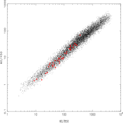
Colour plots: the ratio $S_{450}/S_{850}$

Figure 6 shows the colour-colour plot for $S_{60}/S_{450}$ versus $S_{60}/S_{850}$ for the objects in this sample which have 450$\mu$m fluxes (stars and circles) plus some objects from the literature (which are not in our sample) with fluxes at these wavelengths (IC 1623, NGC 891, Mrk 231, Mrk 273, UGC 5101 – open triangles) plus some of the optically selected galaxies from our as yet incomplete sample (diamonds). The stars refer to objects which we observed and reduced, and the circles are 450$\mu$m fluxes from the literature for this sample.

Figure 6: Colour-colour plot for the objects in the IRAS sample with 450$\mu$m fluxes (stars and circles), other objects from the literature including Mrk 231 (triangles) and some of the optically selected sample (diamonds). The conservative uncertainty in the ratios is shown based on flux error of 10% for 60$\mu$m, 20% for 850$\mu$m and 30% for 450$\mu$m. The best fit line is shown, which has a slope of unity. Data for the stars and open circles is from this paper, triangles from Rigopoulou et al. (1996); Alton et al. (1998); Frayer et al. (1999), and the diamonds are from Dunne (2000)

There are a few points to note here:

1. The relationship is very tight (correlation coefficient $r_{s}=0.96$, significance=$5.8\sigma$) and the scatter is consistent with the uncertainties in the flux ratios (denoted on the figure).

2. This relationship holds across 2–3 orders of magnitude in $L_{\rm{fir}}$, even though there are many different types of galaxies, ranging from optically selected galaxies with low $L_{\rm{fir}}$ to very active ULIRGS and AGN such as Arp 220 and Mrk 231.

3. The best fitting line (least squares) is:

   $$\log(S_{60}/S_{450})=(1.01\pm 0.03)\,\log(S_{60}/S_{850})-(0.909\pm 0.045)$$ (6)

   This can be re-written as $S_{60}/S_{450}=0.123\,(S_{60}/S_{850})^{1.01}$ which implies that, within the uncertainties, the ratio $S_{450}/S_{850}$ is constant. From the fluxes, the mean $S_{450}/S_{850}=7.9$ with $\sigma=1.6$ which is a remarkably tight distribution, consistent with the errors on the fluxes.

What does a constant value of $S_{450}/S_{850}$ mean? The flux ratio can be expressed as a function of $T$ and $\beta$ as follows:

$$\frac{S_{450}}{S_{850}}=\left(\frac{\nu_{450}}{\nu_{850}}\right)^{\beta}\times\frac{{\rm{B}}(\nu_{450},T)}{{\rm{B}}(\nu_{850},T)}$$ (7)

Since the submm fluxes are on the Rayleigh-Jeans side of the Planck function the temperature dependence is not very steep, roughly $\propto T$. A constant value for the ratio therefore implies a small range of real $\beta$ and $T_{c}$ in the ISM of galaxies. We further investigated the implications of the relationship in Fig. 6 in the following way: Hypothetical SEDs were created using the parameters $T_{w}$, $T_{c}$, $N_{c}/N_{w}$ and $\beta$, the values for these being either specified, drawn from a uniform random distribution between two given limits, or drawn from a Gaussian distribution with a designated mean and dispersion. The various models are listed in Table 8. Each SED was used to produce fluxes at 60, 450 and 850$\mu$m. These fluxes were then subjected to ‘observational uncertainties’ by drawing a new flux from the Gaussian distribution with the original flux as the mean and 1$\sigma$ uncertainties derived from the observations as 7, 25 and 14 percent at 60, 450 and 850$\mu$m respectively. Next, only those new fluxes which were found to be $\geq 3$ times the error were selected, to mimic detection limits. The required flux ratios $S_{60}/S_{450}$, $S_{60}/S_{850}$ and $S_{450}/S_{850}$ were then calculated from these final fluxes. In order to be able to compare such things as the linear fitting parameters to those derived from the actual data, we needed to use the same number of data points (37). Therefore fluxes were created in sets of 37, and each set was fitted in exactly the same way as the real data (simple least squares analysis) and the standard deviation on the ratio $S_{450}/S_{850}$ calculated. 10,000 versions of Fig. 6 were created for each SED model, and used to produce an estimate of the mean slope and intercept of the best fitting line and also $\sigma_{450/850}$ (the dispersion on the ratio $S_{450}/S_{850}$). Additionally, one point from each set of 37 was taken and placed into a separate group. These 10,000 flux ratios were then compared with the distribution of the real flux ratios via Kolmogorov-Smirnoff two-sample tests. These points are plotted against the real data for the different models in Fig. 7. We tried different models to see what combination of parameters best reproduced the statistical properties of the data, in particular:

1. the mean values and distributions of the three flux ratios.

2. the best fitting slope and intercept.

3. the dispersion of the flux ratio $S_{450}/S_{850}$.

The models represent a range of ‘realistic’ isothermal and two-component SEDs of the form fitted to the fluxes earlier. One additional model was included to account for the possible contribution of the ¹²CO(3–2) line to the 850$\mu$m filter. This line is excited in warm ($T_{k}>33$ K), dense gas and may comprise a non-negligible fraction of the bolometer flux. Observations of this line are still relatively rare as they are hampered by the same difficult observing conditions which have held continuum observers in the dark for so long. The only accurate way to ascertain the contribution of the line to the 850$\mu$m flux is to map the same galaxies in CO(3–2) and compare the total flux in the line to that in the continuum. Failing this, rough estimates of the CO(3–2) contribution may be made in a variety of ways (see Dunne 2000 for details, also Papadopoulos & Allen 2000; Israel et al. 1999; Bianchi et al. 1998; Mauersberger et al. 1999), all consistent with approximately 4–30 percent of the total continuum flux being due to CO(3–2) line emission. This large range reflects the strong dependence of CO(3–2) on the physical conditions in the gas. CO(3–2) observations of 50 galaxies from the SLUGS IRAS sample are in progress which should allow us to make a better estimate of the contamination in the future (Seaquist, private communication). The effects of possible line contamination are not very large (as the suspected line contribution is comparable to the uncertainty in the submm fluxes) but would lead to us overestimating the dust masses by up to 30 percent and underestimating $\beta$ by $\sim 0.1$ in both the isothermal and two-component temperature cases. To mimick a CO(3–2) contribution Model 7 simply adds 10 percent to the predicted 850$\mu$m flux from the SED template, which has the effect of reducing the flux ratios for a given $\beta$. The tightness of the correlation in Fig. 6 suggests that the contribution by this line adds little to the scatter and is therefore either relatively small or a remarkably constant fraction of the continuum flux. The results of the comparisons of simulations and data are in Table 9.

Table 8: Parameters for SED templates.

Model	$T_{w}$ (K)	$T_{c}$ (K)	$\beta$	$N_{c}/N_{w}$
1	Uni 25 – 65	–	Uni 1–2	–
2	Gau $\mu=35.7$, $\sigma=5.3$	–	Gau $\mu=1.3$, $\sigma=0.2$	–
3	Uni 30–55	Gau $\mu=20$, $\sigma=2.5$	2	Uni 1–100
4	Uni 30–55	18	2	Uni 1–100
5	Uni 30–55	Uni 15–25	1.5	Uni 1–100
6	Uni 30–55	Gau $\mu=20$, $\sigma=2.5$	Uni 1.5–2.0	Uni 1–100
7∗CO	Uni 30–55	Gau $\mu=20$, $\sigma=2.5$	2	Uni 1–100

Table 9: Results of simulations.

(1)	(2)	(3)	(4)	(5)	(6)	(7)	(8)	(9)	(10)
Model	Slope	Int.	$\sigma_{450/850}$	$\langle S_{60}/S_{450}\rangle$	KS	$\langle S_{60}/S_{850}\rangle$	KS	$\langle S_{450}/S_{850}\rangle$	KS
Data	$1.01\pm 0.03$	$-0.909\pm 0.045$	$1.6^{+0.42}_{-0.24}$	$13.9\pm 2.1$		$104\pm 14$		$7.90\pm 0.26$
1	0.915	$-0.684$	$2.67$	64.6	0.52	574	0.49	8.13	0.15
	$3.2\sigma$	$5\sigma$	2.5e-4		2.4e-9		1.9e-8		0.33
2	0.924	$-0.680$	$2.01$	12.9	0.1	89.9	0.13	6.80	0.32
	$2.9\sigma$	$5.1\sigma$	0.079		0.83		0.51		5e-4
3	0.993	$-0.910$	$2.36$	14.6	0.16	124.4	0.09	8.72	0.23
	$0.6\sigma$	$0.02\sigma$	4.1e-3		0.26		0.89		0.03
4	0.987	$-0.881$	$2.22$	15.9	0.18	133.2	0.14	8.34	0.17
	$0.8\sigma$	$0.6\sigma$	0.0137		$0.18$		0.46		0.23
5	0.992	$-0.774$	$1.73$	5.5	0.5	34.2	0.55	6.32	0.42
	$0.6\sigma$	$3.0\sigma$	0.521		8.7e-9		2e-10		2e-6
6	0.970	$-0.808$	$2.14$	9.0	0.33	68.3	0.33	7.47	0.20
	$1.3\sigma$	$2.2\sigma$	0.026		4.3e-4		5.7e-4		0.089
7∗CO	0.992	$-0.869$	$2.15$	14.5	0.16	113.3	0.13	7.92	0.12
	$0.6\sigma$	$0.9\sigma$	0.022		0.26		0.56		0.69

(a) Model 1

(b) Model 2

(c) Model 3

(d) Model 4

(e) Model 5

(f) Model 6

(g) Model 7

Figure 7: Comparison of the 10,000 simulated flux ratios and the actual data points for the 37 galaxies (red stars) for models 1–7.

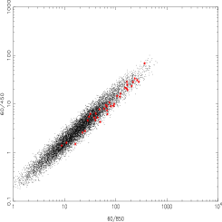
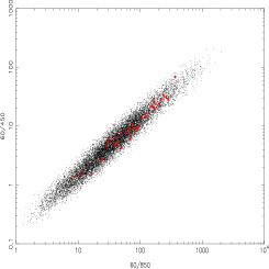
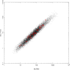
The two isothermal SED models (1 & 2) are not compatible with the data as firstly, the ratio of $S_{450}/S_{850}$ is not predicted to be constant (slope not unity), and secondly the means and distributions of the flux ratios are not compatible with the data and are ruled out by the KS tests at a high level of significance. Not all two-component models can reproduce the observed Fig. 6 either. Models 5 & 6 which have lower $\beta$ values (either $\beta=1.5$ or $\beta$ has a range of values between 1.5–2.0) are also not compatible because their flux ratio predictions are too low (i.e. too much submm flux compared to that at 60$\mu$m), however they do produce the correct slope. The three models which had $\beta=2$ (3, 4 & 7) all produced acceptable matches to the data (the only marginal point being the ratio of $S_{450}/S_{850}$ in Model 3 which had a KS significance of 0.03). Lowering the cold temperature slightly as in Model 4, solved this discrepancy. Also, Model 7, which includes the effect of a CO(3–2) contribution can produce the correct flux ratio with the same cold temperature as Model 3 (i.e. 20 K). While there is an element of $T_{c}$, $\beta$ degeneracy in fitting the ratio $S_{450}/S_{850}$ (we could raise the cold temperature and lower $\beta$ to produce the same ratio), this does not solve the problem with the IRAS/submm ratios which were all significantly different from the data in the lower $\beta$ models. For this reason, we believe that Fig. 6 is evidence in favour of a steep and universal $\beta$ value close to 2. Any CO(3–2) contribution will only strengthen this conclusion and further reject lower $\beta$ values. The warm temperatures used in the models were based on the values which came out of the two-component fits, and were kept constant for all models. We did experiment with altering them but for all realistic scenarios the warm temperature values did not have a significant effect on the models. The same is true for the ratio of cold/warm dust, which was allowed to vary between 1–100 as per the two component fits. The tightness of the ratio $S_{450}/S_{850}$ was very difficult to reproduce with the simulations, and indeed it was not obvious which factors directly affected this. In all cases the models could not reproduce as tight a distribution as the actual data. This may be because we have been too conservative with our estimates of the observational uncertainties, or more likely, because there are intrinsic relationships between such parameters as $T_{w},\,T_{c}$ and $N_{c}/N_{w}$ which were not accounted for in our models.

A cold component temperature between 15–25 K and $\beta\sim 2$ is in good agreement with the measurements of the diffuse ISM in the Galaxy ($T\sim 17$ K, $\beta=2.0$) by COBE/FIRAS (which had enough spectral resolution to do it properly), and with calculations of the predicted equilibrium temperature for grains in the Galactic ISRF which is 25–15 K, depending on Galactocentric distance (Cox, Krügel & Mezger 1986).

The Verdict

From SED fitting alone, it is often not possible to simultaneously determine $\beta$ and to show conclusively that there is a cold dust component, even when as for Arp220 (Fig. 3), there are measurements at many FIR/submm wavelengths. The results of the simulations of the 450/850$\mu$m ratio strongly favour $\beta=2$, and for the 7 galaxies where a cold component is essential (Section 3.3), this is also the $\beta$ value from the fit. We will therefore assume that $\beta=2$ is the true value and that it holds for all galaxies. Since there is abundant evidence in the literature for both cold components and $\beta\sim 2$ we accept it as the best physical model for the SED. Acceptable two-component fits using $\beta=2$ were possible for all of the sources.

4 Discussion

The galaxies were re-fitted using Eqn. 5 but now assuming a fixed $\beta=2$. The results are given in Table 10 and some examples of the fits are shown in Fig. 8.

(a) ugc903: $T$(45,21), n=91

(b) ngc958: $T$(44,20), n=186

(c) ugc2369: $T$(36,21), n=6

(d) ugc2403:$T$(50,22), n=100

(e) ir1211: $T$(49,24), n=27

(f) ngc1667: $T$(28,17), n=3

(g) ugc2982: $T$(31,17), n=6

(h) ir1525: $T$(45,19), n=15

(i) ugc5376: $T$(44,21), n=87

(j) ngc2623: $T$(50,27), n=18

(k) arp220: $T$(48,18), n=42

(l) ngc7592: $T$(39,19), n=20

Figure 8: Two-component SEDs assuming $\beta=2$ for IRAS sample. The solid lines represent the composite 2-component SED while the dot-dash lines show the warm and cold components. The caption to each figure gives the two temperatures plus the ratio of cold:warm dust (n).

Table 10: Temperatures and dust masses for two-component SEDs assuming $\beta=2$.

(1)	(2)	(3)	(4)	(5)	(6)	(7)	(8)	(9)	(10)	(11)
Name	$T_{w}$	$T_{c}$	$\frac{N_{c}}{N_{w}}$	$M_{\rm{d2}}$	$R_{M}$	$L_{\rm{fir}}$	$R_{L}$	$G_{\rm{d(HI)}}$	$G_{\rm{d(H2)}}$	$G_{\rm{d}}$
	(K)	(K)		(log $\rm{M_{\odot}}$)		(log $\rm{L_{\odot}}$)
UGC 903	45	21	91	7.37	1.95	10.34	1.17	141	…	…
NGC 520	50	24	61	7.46	1.74	10.78	1.12	204	234	438
NGC 958	44	20	186	8.28	1.86	11.04	1.17	204	85	289
UGC 2369	36	21	6	8.08	2.04	11.34	1.02	…	269	…
UGC 2403	50	22	100	7.57	2.04	10.71	1.17	…	…	…
UGC 2982	31	17	6	8.11	2.34	10.99	1.00	91	132	223
NGC 1614	38	20	3	7.78	2.14	11.32	1.00	58	174	232
NGC 1667	28	17	3	7.91	1.82	10.81	1.00	69	117	186
NGC 2623	50	27	18	7.59	1.58	11.36	1.07	46	240	286
NGC 2856	45	22	58	7.08	1.91	10.23	1.12	117	…	…
NGC 2990	42	21	58	7.33	1.91	10.35	1.12	229	…	…
UGC 5376	44	21	87	7.11	1.91	10.05	1.12	200	…	…
NGC 3110	42	23	44	7.93	1.58	11.10	1.10	…	257	…
IR 1017+08	40	19	8	8.20	2.95	11.52	1.10	…	151	…
IR 1056+24	40	26	6	8.14	1.51	11.79	1.02	…	166	…
Arp 148	37	21	12	8.28	2.09	11.41	1.05	…	85	…
MCG+00-29-023	36	20	13	7.99	2.14	11.04	1.05	…	…	…
IR 1211+03	49	24	27	8.55	2.29	12.05	1.12	…	123	…
NGC 4418	58	21	62	7.40	3.47	10.77	1.15	22	52	74
UGC 8387	33	24	2	7.92	1.29	11.39	1.00	…	148	…
Zw 247.020	39	25	6	7.50	1.51	11.04	1.02	…	…	…
Zw 049.057	44	23	28	7.74	1.82	11.05	1.07	…	65	…
1 Zw 107	39	20	7	8.23	2.63	11.56	1.02	…	93	…
IR 1525+36	45	19	15	8.29	3.98	11.69	1.00	…	…	…
Arp 220	48	18	42	8.80	3.24	11.95	1.02	48	41	89
NGC 5962	31	18	11	7.49	2.19	10.26	1.17	98	120	218
NGC 6052	37	20	16	7.65	2.14	10.72	1.07	170	85	255
NGC 6181	31	19	7	7.47	1.86	10.39	1.05	191	195	386
NGC 7541	31	17	6	7.90	2.40	10.77	1.02	195	112	307
NGC 7592	39	19	20	8.13	2.75	11.14	1.05	87	129	216
NGC 7679	37	19	14	7.75	2.51	10.81	1.05	112	…	…
NGC 7714	42	21	13	7.05	2.34	10.39	1.05	151	191	342
							mean	128	142	253

Gas and dust masses

The dust mass has to be re-calculated if a colder component is present, and will always be higher than if only one temperature is assumed. The two-component dust mass is calculated as follows:

$$M_{d2}=\frac{S_{850}\,D^{2}}{\kappa_{d(850)}}\times\left[\frac{N_{c}}{{\rm{B}}(850\mu m,\,T_{c})}+\frac{N_{w}}{{\rm{B}}(850\mu m,\,T_{w})}\right]$$ (8)

where $\kappa_{d(850)}$ is assumed to have the same value as in Paper I (0.077 m² kg^-1). It is the temperature of the colder component which is critical for an accurate determination of the dust mass as it is this dust component which produces most of the emission at 850$\mu$m. If $T_{c}$ has been overestimated then the dust mass will be underestimated, in much the same way as if only a single temperature had been assumed. The FIR luminosity can easily be integrated under the new two-component SED and this and the dust masses are given in Table 10, along with the revised gas-to-dust ratios. On average, the dust masses increase by a factor $\sim 2$ compared to the single temperature estimates from Paper I. In contrast, the values of $L_{\rm{fir}}$ do not increase by much at all and this is simply because the long wavelength region, where the cold component has modified the SED, does not contribute much to the integrated energy. The gas-to-dust ratios are also lower than in our earlier paper by a factor $\sim 2$, bringing them more into line with the Galactic value of 226 (Sodroski et al. 1997). There is a slight tendency for the galaxies with the largest angular sizes to have higher gas-to-dust ratios (NGC 520, NGC 958, NGC 6181, NGC 7541) which could be due to us missing some extended dust emission outside the region mapped by SCUBA.

Figure 9: Dust mass functions. Solid line:– ‘cold dust mass’ function, dust masses are from Table 10 and from Paper I using a second cold component with $T_{\rm{c}}=20\,\rm{K}$ and $\beta=2$. Dashed line – dust masses calculated from the 850$\mu$m fluxes using a single temperature as in Paper I. Schechter parameters shown are $\alpha=-1.85$, $M_{\rm{d2}}^{\ast}=9.3\times 10^{7}$ M_⊙ and $\phi^{\ast}=4.9\times 10^{-4}$ Mpc^-3 dex${-1}$ (solid); $\alpha=-1.23$, $M_{\rm{d}}^{\ast}=2.5\times 10^{7}$ M_⊙ and $\phi^{\ast}=1.6\times 10^{-3}$ Mpc^-3 dex^-1 (dashed).

For the galaxies without useful 450$\mu$m data, one can obtain reasonable estimates of dust mass by fitting a two-component model with $T_{c}$ and $\beta$ fixed at 20 K and 2. This is actually the procedure used in Paper I to investigate the possibility of cold dust. The dust mass function for the whole sample using the dust masses derived in this paper and those ‘cold dust masses’ ($M_{\rm{d2}}$) given in Table 4 of Paper I is shown in Fig. 9. This function could still be an underestimate if there are large numbers of cold, dusty galaxies which are not present in the IRAS sample.

4.1 Dust heating

Figure 10: Distribution of cold temperatures using $\beta=2$.

The new distribution of $T_{c}$ is shown in Fig. 10 and is now much tighter than when $\beta$ was not fixed; it is also more Gaussian with a single peak at 21 K. The mean is 20.9 K with $\sigma=2.5$, and both the mean value and the small spread agrees with the range of values for $T_{c}$ found in the literature (15 – 25 K:- Haas et al. 1998,2000; Frayer et al. 1999; Braine et al. 1997; Dumke et al. 1997; Calzetti et al. 2000; Guélin et al. 1995; Sievers et al. 1994; Neininger et al. 1996; Alton et al. 1998). It is also interesting to note that alternative approaches to the SED inversion problem presented by Pérez Garcia et al. (1998) and Hobson et al. (1993) also require two or more temperature components and produce similar temperatures. When observations are made with enough spatial resolution, the SEDs of the central and outer regions of a galaxy can be fitted separately. This often shows that the central regions contain most of the warm dust at $T>30$ K while the outer disk regions are dominated by the colder ($15-20$ K) dust, the total SED being the sum of the inner and outer (Papadopoulos & Seaquist 1999; Haas et al. 1998; Dumke et al 1997; Braine et al. 1997; Trewhella et al. 2000). This suggests that $N_{c}/N_{w}$ (or the prominence of the cold component) is really telling us about the relative importance of the disk/bulge dust components in these galaxies (similar to the cirrus/starburst components in the models of Rowan-Robinson & Crawford 1989). The more active starburst galaxies in the sample display conditions like the centres of normal galaxies over a much larger region, so that the central warmer component dominates the SED. The fact that the warm dust always out-shines the cooler dust (per unit mass) is what makes it so difficult to disentangle the cold component from the SED in cases where there is a relatively large amount of warm dust.

The equilibrium temperature of a dust grain immersed in a radiation field can be expressed as a function of the interstellar radiation field (ISRF) as (van der Hulst 1946; Disney et al. 1989)

$$T_{\rm{eq}}\propto\rm{ISRF}^{1/5}$$

This would lead one to expect variations in $T_{c}$ if some galaxies (e.g. the more active starbursting ones) have higher ISRFs – leading to slightly warmer grain temperatures in their diffuse, cold component. The range of $T_{c}$ found in these galaxies (17–27 K) corresponds to a factor of $\sim 10$ in ISRF intensity, although it may have been expected that the more active star forming galaxies in the sample would have ISRFs many orders of magnitude greater than that in the Milky Way. However, these active environments are also localised and dusty, therefore a lot of the extra short wavelength stellar radiation (UV) may be absorbed near to the source, producing enhanced FIR radiation which is in fact the warm component. It is generally believed that older stars contribute significantly to the heating of the diffuse ‘cirrus’ dust component as well as some radiation from OB stars which leaks from the star forming molecular clouds, although the relative importance of OB stars as a source of heating is still not well determined (Bothun, Lonsdale & Rice 1989; Cox, Krügel & Mezger 1986; Walterbos & Greenawalt 1996; Boulanger & Perault 1988). If OB radiation leaked from sites of star formation is not an important heating source for the colder component then the distribution of older stars and diffuse dust must be responsible for any changes in $T_{c}$. We will leave an investigation of the details of the dust heating to a future paper.

Figure 11: 60$\mu$m luminosity correlated with dust temperature (from isothermal models) in Paper I.

(a) Warm temperature vs. $L_{60}$.

(b) Warm ‘energy’ vs. $L_{60}$.

Figure 12: a) Using the warm component temperature $T_{w}$, there is no longer a relationship with $L_{60}$. b) Creating a warm ‘energy’ by combining $T_{w}$ with the ratio of cold/warm grains, there is now a correlation with $L_{60}$.

(a) Dust mass vs. $L_{60}$.

(b) Warm ‘luminosity’ vs. $L_{60}$.

Figure 13: a) Dust mass (using the two-component parameters) does correlate with $L_{60}$, but the slope is less than unity meaning there must be some other contribution to $L_{60}$ than mere size. b) Combining dust mass with the warm ‘energy’ to produce a distant dependent quantity (termed warm ‘luminosity’) gives a remarkably tight relationship with $L_{60}$ which does have a slope of unity.

(a) Cold ‘energy’ vs. $L_{60}$

(b) Cold ‘luminosity’ vs. $L_{60}$.

Figure 14: a) Creating an analogous cold ‘energy’ using $T_{c}$ and $N_{c}/N_{w}$ does not correlate at all with $L_{60}$ in contrast to Fig. 12b. b) Multiplying the cold ‘energy’ by dust mass to create the cold luminosity is only barely dependent on $L_{60}$ via the relationship between dust mass and luminosity. This highlights the significance of the strong relationship in Fig. 13b.

Table 11: Parameters for fits and correlations

$y$	$x$	$r_{s}$	Prob	$\sigma$	linear fit: $y=mx+c$
					$m$	$c$
$T_{\rm{d}}$	log $L_{60}$	0.44	$2.5e-6$	4.7	$4.57\pm 0.82$	$-71.9\pm 19.4$
$T_{\rm{w}}$	log $L_{60}$	$0.08$	0.42	0.8	..	..
log [$N_{w}/N_{c}\times T_{\rm{w}}^{6}$]	log $L_{60}$	$0.62$	2.1e-12	6.3	$0.735\pm 0.068$	$-9.04\pm 1.25$
log $M_{\rm{d2}}$	log $L_{60}$	0.83	$2.7e-27$	8.4	$0.727\pm 0.036$	$-9.31\pm 0.70$
log [$M_{\rm{d2}}\times(N_{w}/N_{c})T_{w}^{6}$]	log $L_{60}$	0.98	0.0	9.9	$1.018\pm 0.014$	$-7.95\pm 0.29$
log [$N_{c}/N_{w}\times T_{\rm{c}}^{6}$]	log $L_{60}$	0.16	0.40	0.8	..	..
log [$M_{\rm{d2}}\times(N_{c}/N_{w})T_{c}^{6}$]	log $L_{60}$	0.35	0.053	1.9	..	..

In Paper I we presented a relationship between dust temperature (as fitted by an isothermal model) and 60$\mu$m luminosity (Fig. 11). Our explanation for this was that the position of the 60$\mu$m flux on the Wien side of the Planck function makes it very sensitive to dust temperature. For a given mass of dust, hotter galaxies would be easier to detect in a 60$\mu$m flux limited sample and therefore a dependence of 60$\mu$m luminosity on dust temperature is observed. We can now investigate this further using the extra information we have about how the dust is split into warm and cool components. The correlation coefficients and fits to the following relationships are detailed in Table 11. We will now use the whole data set of 104 galaxies. Those galaxies without useful 450$\mu$m data were fitted with a two-component model using fixed $\beta=2$ and $T_{c}=20$ K (as described in Paper I). Fig. 12a shows that there is no correlation between the fitted warm temperature and 60$\mu$m luminosity. The quantity which is important now is the proportion of energy in the warm component, which can be described roughly as $(N_{c}/N_{w})^{-1}\times T_{w}^{6}$. This has a quite a strong relationship with $L_{60}$ as displayed in Fig. 12b, although there is a lot of scatter. This relationship is not linear, having a slope less than unity. It must be remembered here that luminosity is a distant dependent quantity but the relative amount of ‘warm energy’ is not as it has not been normalised in any way to the galaxy size. Is there a strong connection between galaxy size (or dust content) and $L_{60}$? In Paper I we argued that the link between dust temperature and $L_{60}$ was not a function of galaxy size (i.e. dust temperature and dust mass were unrelated, which is still the case here). However, dust mass and $L_{60}$ are clearly related as shown in Fig. 13a although the relationship is not linear either (slope is less than unity) and therefore 60$\mu$m luminosity would seem to depend on both the quantity of dust in the galaxy and the relative amount of energy in the warm component. If the ‘warm energy’ quantity from Fig. 12b is multiplied by $M_{\rm{d2}}$ to produce a distant dependent variable similar to $L_{60}$ we find a remarkably tight correlation between this product, the ‘warm luminosity’, and the 60$\mu$m luminosity (Fig. 13b) and the slope of this correlation is unity. Thus the typical FIR luminous objects detected by IRAS do not necessarily have to have vastly more dust than lower luminosity ones, but they do have to have a greater fraction of it heated to warmer temperatures. We can repeat this comparison using the ‘cold energy’ $(N_{c}/N_{w})\times T_{c}^{6}$ and ‘cold luminosity’ $(N_{c}/N_{w})\times T_{c}^{6}\times M_{\rm{d2}}$. Neither of these quantities correlate with $L_{60}$ as shown in Fig. 14. This is an interesting point because if there are galaxies which possess very dominant cold components, even though they may have large quantities of dust, they will not necessarily have large 60$\mu$m luminosities. This means they may not be part of 60$\mu$m flux limited samples and hence represent a population so far absent from our luminosity and dust mass functions. This issue must await the completion of data analysis from our optically selected sample, which should not be biased against galaxies with large fractions of colder rather than warmer dust.

5 Conclusions

We have used our own SCUBA 450$\mu$m data and fluxes from the literature to produce better constraints on the FIR/submm SEDs of the SLUGS IRAS sample. It was often not possible to find unique decompositions of the SEDs using a series of modified Planck functions, either cold temperatures and steep $\beta$ or higher temperatures and lower $\beta$ being equally acceptable. However, by the fact that the 450/850$\mu$m flux ratio is remarkably constant from extreme objects like Arp220 to lower luminosity galaxies we concluded the dust emissivity index $\beta$ could be constrained to be $\sim 2$. Using this value for $\beta$, a colder component is required in most of the sample, but with a very large variation in its contribution. The cold component has a similar temperature in all of the galaxies ($T_{\rm{av}}=21$ K), in agreement with those determined by many other authors in the literature. The dust masses derived using the new temperatures are higher the previous estimates (which used a single-temperature SED) by a factor $\sim 2$, and this brings the gas-to-dust ratios into agreement with that of the Milky Way, and other evolved spiral galaxies. The 60$\mu$m luminosity was found to depend on both dust mass and the relative amount of energy in the warm component, but it has no relationship with the cold component. Galaxies where the cold component is very dominant may not be well represented in 60$\mu$m flux limited samples.

The support of PPARC is gratefully aknowledged by L. Dunne, S. Eales. We also thank the JCMT staff especially Wayne Holland and Iain Coulson for advice on 450$\mu$m calibration. We appreciate useful discussions with Paul Alton.

References

- [1] Agladze N. I., Sievers A. J., Jones S. A., Burlitch J. M., Beckwith S. W., 1996, ApJ, 462, 1026
- [2] Alton P. B., Bianchi S., Rand R. J., Xilouris E., Davies J. I., Trewhella M., 1998, ApJL, 507, L125
- [3] Alton P. B., Lequeux J., Bianchi S., Churches D., Davies, J. Combes F., 2001, A&A, 366, 451
- [4] Archibald E. N, Wagg J. W., Jenness T., 2000, SCD system note 1.1
- [5] Avni Y., Bahcall J. N., 1980, ApJ, 235, 694
- [6] Benford D. J., Cox P., Omont A., Phillips T. G., McMahon R. G., 1999, ApJ, 518, L65
- [7] Bianchi S., Alton P. B., Davies J. I., Trewhella M., 1998, MNRAS, 298, L49
- [8] Bothun G. D., Lonsdale C. J., Rice W., 1989, ApJ, 341, 129
- [9] Boulanger F., Perault M., 1988, ApJ, 330, 964
- [10] Braine J., Guélin M., Dumke M., Brouillet N., Herpin F., Wielebinski R., 1997, A&A, 326, 963
- [11] Braine J., Dumke M., 1998, A&A, 333, 38
- [12] Calzetti D., Armus L., Koorneef J., Storchi-Bergmann T., 2000, ApJ, 533, 682
- [13] Carico D. P., Keene J., Soifer B. T., Neugebauer G., 1992, PASP, 104, 1086
- [14] Chini R., Kreysa E., Krügel E., Mezger P. G., 1986, A&A, 166, L8
- [15] Chini R., Krügel E., Kreysa E., Gemuend H.-P., 1989, A&A, 216, L5
- [16] Chini R., Krügel E., 1993, A&A, 279, 385
- [17] Chini R., Krügel E., 1994, A&A, 288, L33
- [18] Cox P., Krügel E., Mezger P. G., 1986, A&A, 155, 380
- [19] Davies J. I., Alton P., Trewhella M., Evans R., Bianchi S., 1999, MNRAS, 304, 495
- [20] de Jong T., Brink K., 1987, in Persson C. J., ed, Star Formation in Galaxies, NASA, Washington, p. 323
- [21] Devereux N. A., Young J. S., 1990, ApJ, 359, 42
- [22] Disney M. J., Davies J. I., Phillipps S., 1989, MNRAS, 239, 939
- [23] Downes D., Radford S. J. E., Greve A., Thum C., Solomon P. M., Wink J. E., 1992, ApJ, 398, L25
- [24] Downes C., Solomon P. M., 1998, ApJ, 507, 615
- [25] Draine B. T., Lee H. M., 1984, ApJ, 285, 89
- [26] Dumke M., Braine J., Krause M., Zylka R., Wielebinski R., Guélin M., 1997, A&A, 325, 124
- [27] Dunne L., 2000, PhD. thesis, Cardiff College, University of Wales.
- [28] Dunne L., Eales S. A., Edmunds M. G., Ivison R. J., Alexander P., Clements D. L., 2000, MNRAS, 315, 115. (Paper I).
- [29] Dunne L., 2001, in prep
- [30] Dupac X. et al., 2001, ApJ in press (astro-ph/0102407)
- [31] Eales S. A., Wynn-Williams C. G., Duncan W. D., 1989, ApJ, 339, 859
- [32] Fox M., 2000, PhD. thesis, Imperial College, University of London.
- [33] Frayer D. T., Ivison R. J., Smail I., Yun M. S., Armus L., 1999, AJ, 118, 139
- [34] Gordon M. A., 1988, ApJ, 331, 509
- [35] Gordon M. A., 1995, A&A, 301, 853
- [36] Guélin M., Zylka R., Mezger P. G., Haslam C. T., Kreysa E., 1995, A&A, 298, L29
- [37] Jenness T., Lightfoot J. F., 1998, Starlink User Note (SUN) 216.4
- [38] Haas M., 1998, A&A, 337, L1
- [39] Haas M., Klaas U., Coulson I., Thommes E., Xu C., 2000, A&A, 356, L83
- [40] Hobson M. P., Padman R., Scott P. F., Prestage R. M., Ward-Thomson D., 1993, MNRAS, 264, 1025
- [41] Huchra J., Davis M., Latham D., Tonry J., 1983, ApJS, 52, 89
- [42] Hughes D. H., Dunlop J. S., Rawlings S., 1997, MNRAS, 289, 766
- [43] Israel F. P., van der Werf P. P., Tilanus R. P. J., 1999, A&A, 344, L83
- [44] Ivison R. J. et al., 1998, ApJ, 494, 211
- [45] Klaas U., Haas M., Heinrichsen I., Schulz B., 1997, A&A, 325, L21
- [46] Knapp G. R., Sandell G., Robson E. I., 1993, ApJS, 88, 173
- [47] Krügel E., Siebenmorgen R., 1994, A&A, 288, 929
- [48] Lonsdale Persson C. J., Helou G., 1987, ApJ, 314, 513
- [49] Masi S. et al., 1995, ApJ, 452, 253
- [50] Mathis J., Whiffen G., 1989, ApJ, 341, 808
- [51] Mauersberger R., Henkel C., Walsh W., Schulz A., 1999, A&A, 341, 256
- [52] Mennella V., Colangeli L., Bussoletti E., 1995, A&A, 295, 165
- [53] Mennella V., Brucato J. R., Colangeli L., Paulmbo P., Rotundi A., Bussoletti E., 1998, ApJ, 496, 1058
- [54] Neininger N., Guélin M., García-Burillo S., Zylka R., Wielebinski R., 1996, A&A, 310, 725
- [55] Papadopoulos P. P., Seaquist E. R., 1999, ApJ, 514, L95
- [56] Papadopoulos P. P., Allen M. L., 2000, ApJ, 537, 631
- [57] Pérez García A. M., Rodríguez Espinosa J. M., Santolaya Rey A. E., 1998, ApJ, 500, 685
- [58] Reach W. T. et al., 1995, ApJ, 451, 188
- [59] Rigopoulou D., Lawrence A., Rowan-Robinson M., 1996, MNRAS, 278, 1049
- [60] Ristorcelli I. et al., 1998, ApJ, 496, 267
- [61] Roche P. F., Chandler C. J., 1993, MNRAS, 265, 486
- [62] Rowan-Robinson M., Crawford J., 1989, MNRAS, 238, 523
- [63] Sandell G., 1997, Starlink Cookbook 11.1
- [64] Sanders D. B., Scoville N. Z., Soifer B. T., 1991, ApJ, 370 158
- [65] Siebenmorgen R., Krügel E., Chini R., 1999, A&A, 351, 495
- [66] Sievers A. W., Reuter H.-P., Haslam C. T., Kreysa E., Lemke R., 1994, A&A, 281, 681
- [67] Sodroski T. J., Odegard N., Arendt R. G., Dwek E., Weiland J. L., Hauser M. G., Kelsall T., 1997, ApJ, 480, 173
- [68] Soifer B. T., Boehmer L., Neugebauer G., Sanders D. B., 1989, AJ, 98, 766
- [69] Trewhella M., Davies J. I., Alton P. B., Bianchi S., Madore B. F., 2000, ApJ, 543, 153
- [70] van der Hulst H. C., 1946, Rech. Astron. Obs. Utrecht, 11, 1
- [71] Walterbos R. M., Greenawalt B., 1996, ApJ, 460, 696
- [72] Weintraub D. A., Sandell G., Duncan W. D., 1989, ApJ, 340, L69
- [73] Woody D. P. et al., 1989, ApJ, 337, L41
- [74] Wright E. L., 1987, ApJ, 320, 818