MEASUREMENTS OF THE GRAVITY WAVES VELOCITY

Abstract

Some results are presented of the Earth s microseismic background. It is assumed that background peaks should correspond to the resonance gravity-wave exchange in the system of two gravity-connected bodies. The microseismic spectrum is compared with the distribution of gravity potential of the nearest stars. A close peak-to-peak correspondence is found. This correspondence and resonance condition lead to an evaluation of the gravity-wave velocity. The resulting value is nine orders of magnitude more than the velocity of light. Some consequences of such result are discussed.

Introduction

The observational data presented of the Earth s microseismic background associated with gravitational waves shows an influence of the nearest cosmic objects on the Earth. I will use the simplest theoretical model to avoid complexities that might arise in a more sophisticated approach. Let us focus on two gravity-connected objects such as Earth-Moon, Earth-Jupiter, Earth-Saturn, Earth-Sun, Earth-nearest stars. These coupled pairs will be considered as antenna and the whole earth as receiver or sensor. Now if the gravity wave length is comparable with the antenna dimension (the distance $L$ between the gravity-connected objects), resonance phenomena may appear in the antenna, producing a peak in the microseismic background spectrum.

The source of the gravity waves with different frequencies in Univers may be the gravity waves exchange between gravity-connected objects and gravity instability of the cosmic clouds that leads to the stars formation. It is possible to show as an example mechanism of the gravity waves generation with broad frequency spectrum. There is a theorem: if some system can have the position of the unstable equilibrium between stable state and unstable one then this system can oscilate in stable area with low frequencies and this frequencies decreases when the system approaches to the equilibrium (threshold of the instability) with wavenumber being finite at zero frequency [1, 2]. This theorem is aplicable exactly to the case of the gravity instability clouds in Universe. This well known Jeans’s instability lead usually to the process of the stars formation [3]. Presented process must be preceded by the intensive gravity waves creation and spectrum of this waves will continuosly shifts in low frequancy range when clouds will aproach to the instability threshold. Consequently we can state that the gravity waves with different frequencies are existing in Univers allways as the stars creation process is existing allways.

It is possible to evaluate the gravity wave velocity $C$ using the simplest relation between frequency $\nu$ and wavelength $\lambda$, i. e., $\nu=C/\lambda$ (assuming $\lambda/2\sim L$) if such peaks are observed. Consequently, the goal of this study of the microseismic background is to search for such peaks.

Observations

Our observations were made in the seismic station at Simpheropol University at Sevastopol using laser interferometery [4]. Six peaks were found at $2.3Hz$, $1Hz$, $0.9Hz$, $0.6Hz$, $0.4Hz$, $0.2Hz$ (see Fig.1 $a$, $b$). These figures were taken directly from the spectranalyser SK4-72 using recording equipment. The SK4-72 accumulates the output interferometer signals and enhances the periodic components of the signal relative to chaotic components. One thousand twenty four records of length 40 seconds were averaged.

There exist massive gravity objects at distances of 1.3, 2.7, 3.5, 5, 8, and around 11 parsecs. All the distances $L$ between earth and these objects correspond to all the observed peaks only if the value of the gravity-wave velocity $C$ is nearly nine orders of magnitude greater than the velocity of light, if we ascribe

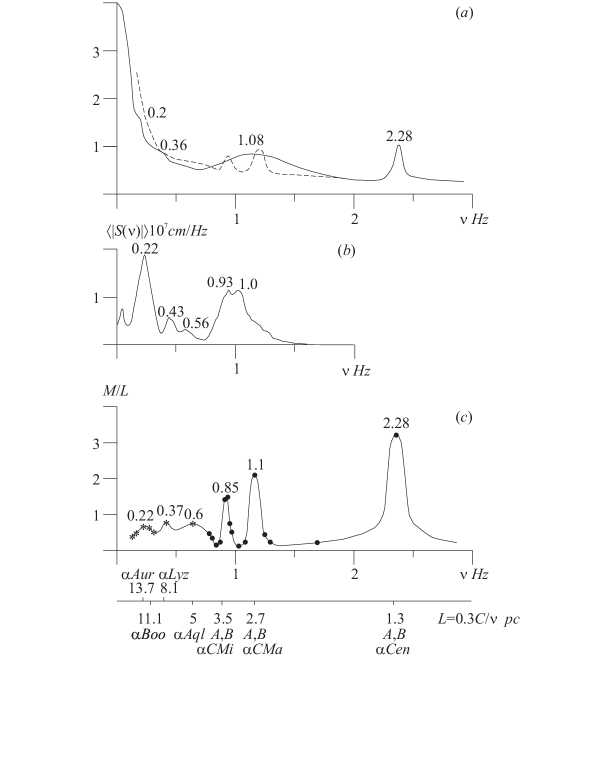
Figure 1: Observed microseismic background (solid curve) after accumulation of the background signals from the interferometer output: $a$) - the $0.1-5Hz$ range; $b$) the $0.1-2Hz$ range. The dotted curve on a) shows the calculated distribution of the stars gravity potential plus the uniform part of the microseismic background. This dotted curve is normalized so as to equalize the value of the dotted and solid curves at $2.28Hz$. $c$) - the calculated distribution of the stars gravity potential. The solid points correspond to all nearest stars with distances $L<4$ parsecs, and the stars to all brightest stars for which $L>4$ parsecs. Mass $M$ is in sun masses. $\alpha Aur-\alpha Cen$ means $\alpha$ stars of the constellation in standard astronomical notation [5, 6]. $A$, $B$ signifies star doublets. The numbers at the extremal curve points are frequencies.

them to resonances in the earth-object system in accord with the simple formula $\nu=C/\lambda$ ($\lambda/2\sim L$ due to resonance). This conclusion permits the calculation of the gravity-potential distribution of the nearest stars. This distribution is shown in Fig.1 $c$. Comparison of Fig.1 $a$, $b$ with Fig.1 $c$ reveal a close similarity of corresponding curves: each peak of Fig.1 $a$, $b$ corresponds to a peak on Fig.1 $c$ and vice versa. However, there are non-important differences that should be pointed out for clarity. For distances $L>4$ parsecs, data were taken only for the brightest star, and the curve of gravity potential corresponding to this distance is lower than for the $L<4$ level on the theoretical Fig.1 $c$. Another difference consists of the presence of uniform growth for the low-frequency background component on experimental Fig.1 $a$, $b$ which does not appear on Fig.1 $c$. Usually this uniform component of the microseismic background is described by the law $A_{\omega}\sim 1/\omega^{2}$ [7, 8].

Besides the quantitative correlation of frequency peaks with the distribution of the nearest stars, there is qualitative correspondence as well. Namely, the sharpest peak at $2.28Hz$ corresponds mainly to the distance between earth and the nearest stars doublet $A$ and $B$ ($\alpha$ Centaurus [5, 6]). The broader peak at $1Hz$ on Fig.1 $a$, $b$ corresponds to the distances to stars distributed over the range from 2.4 to 3.8 parsecs [5, 6]. The spectranalyzer SK4-72 averages all resonance peaks for this $2.4-3.8$ range into one broad peak around $1Hz$ (Fig.1 $a$). But the broad peak on Fig.1 $a$, under more careful study, splits into two peaks (Fig.1 $b$) if spectranalyzer SK4-72 is processing in the frequency range from $0.1$ to $2Hz$ (the exaggeration of the frequency scale). This subdivision of the frequency range corresponds to the divisions of the group of stars from 2.4 to 3.8 parsecs into two subgroups situated around 2.7 and 3.5 parsecs (Fig.1 $c$).

The gravity potential distribution of these subgroups plus the uniform background spectrum is shown on Fig.1 $a$ by the dotted curve. Thus we see both quantitative and qualitative correlation of the frequency spectra of the microseismic background that can be associated with resonance gravity-wave exchange. It is these correlations that provide the possibility of evaluating the gravity-wave velocity which turns out to be nine orders of magnitude greater than the velocity of light.

If the experimental results are considered to be meaningful then it is possible to propose further more decisive observations. Namely, it is reasonable to look for resonance peaks corresponding to the gravitational wave exchange of the Earth with the Moon ($\sim 240MHz$), the Sun ($\sim 0.6MHz$), Venus ($\sim 0.3-2.2MHz$), Jupiter ($\sim 100-150kHz$), and Saturn ($\sim 58-72kHz$). Moreover, the peaks corresponding to Venus, Jupiter and Saturn should change their frequency in accordance with the changing distance between Earth and these planets during their orbital motion around the Sun. Establishing such a correlation will be a crucial experiment, decisively supporting the results presented above concerning the enormous gravity-wave velocity and the elastic model of the physical vacuum [9].

Discussion

Such enormous velocity gravity waves were discussed before from a different physical perspective [10, 11, 12] and [9]. Laplace gave a lower-limit evaluation of the gravity propagation velocity using observational data on the stability of the Earth-Moon system. This lower limit was found to be $5\cdot 10^{8}$ times greater than the velocity of light $c$ [12]. If we normalize the gravity velocity in Laplace s formula to that of the light velocity, then we get the unacceptable conclusion that the Earth-Moon system could exist only about 3000 years. The gravity-wave velocity evaluation was given independently using theoretical assumptions about the elastic model of the physical vacuum in [9] also. This evaluation of the velocities ratio is close to that of Laplace and is approximately equal to $(e/mf^{1/2})^{1/2}$ where $f$, $e$, and $m$ are the gravitational constant, the electron charge and the proton mass [9]. I did not know of Laplace s result when [9] was written, and therefore a citation to Laplace s result is absent from that paper.

Some problems appearing in connection with the huge gravity-wave velocity are discussed in [9] on the basis of the elastic model of the physical vacuum. The very large difference of the gravity and electromagnetic velocities means, first of all, that many electromagnetic and gravitational phenomena are practically independent and their mutual influence appears only through their appearance in some physical constants. This huge gravity-wave velocity also means that we are living in a practically static gravitational field. Retardation effects become substantial only for distances comparable with the dimensions of the Universe, or for very large cosmic objects at least. This point of view lends a better understanding to the problems of Universe structure and its evolution, as the interaction time between the components of the Universe is considerably less than its lifetime, i. e., components of the Universe are causally connected and we do not need to violate any thermodynamic laws. The existence of a velocity that is larger than the light velocity violates, of course, the relativistic invariance of special relativity theory. But this violation causes only small changes in values of the physical constants (for example, $e$) only in the eighteenth decimal, as in the relativistic root $(1-(v/C)^{2})^{1/2}$ appearing in the elastic model of the physical vacuum [9], the ratio $v/C$ does not exceed $c/C\sim 10^{-9}$ in the approach discussed. In the elastic model, shear waves compare with electromagnetic waves, longitudinal waves with gravitational waves, and the particles are considered as singularities of the elastic body. From the point of view of the singularity, the elastic body is emptiness. Consequently the problem of their capture does not appear. Every singularity has an eigenfrequency spectrum with complex frequencies [13, 9, 14]. The real part of the frequency is connected with the self energy (mass) and the imaginary part determines the lifetime. Consequently, each spectrum mode has eigenfrequency and eigenattenuation, i.e., self energy and lifetime are interconnected. So, we could in principle set up the mathematical problem of the elementary particle mass spectrum as a problem of the inhomogeneity self oscillations the elastic body with the above-mentioned difference of shear and longitudinal velocities having eigenfrequencies $10^{9}$ times more than eigenattenuation [13]. Consequently, our model of the physical vacuum can explain the slow decay of elementary particles [9] if this decay process includes radial self-oscillation of the cavity (model of vacancy). This is one more consequence of the large longitudinal wave velocity of elastic ether and consequently the large gravity wave velocity. The elastic model of the physical vacuum also predicts conversion of gravity waves into electromagnetic waves and vice-versa. Again, the very large ratio of gravity to electromagnetic velocity prevents intensive energy transfer between gravitational and electromagnetic phenomena, as the coefficient of transformation is proportional to $\sim 10^{-9}$. Only for very large-scale phenomena can transformation effects become important: for example, only between gravity-connected large-scale objects can there be intensive gravity-electromagnetic wave exchange that would lead to creation of a photon background. And this electromagnetic background could have footprints of the resonance gravity-wave exchange similar to the microseismic background peaks discussed above. There are, of course, other effects associated with the large difference between the gravity and electromagnetic wave velocities. But these are subjects of further study. At the end, it should be noted that the existence of a gravitational-wave velocity nine orders of magnitude greater than the electromagnetic wave velocity may lead to vast theoretical and experimental consequences and to a better understanding of nature.

References

- [1] Dubrovskiy, V. A., Tectonic waves, Izvestiya, Physics of the Solid Earth, 21, N1, 1985.
- [2] Dubrovskiy, V. A., and Sergeev, V. N., Physics of tectonic waves. Izvestiya, Physics of the Solid Earth, 33, N10, 1997.
- [3] Jeans, J., Astronomy and cosmology, Cambridge Univ. Press, 1928.
- [4] Nesterov, V. V., Longbase laser interferometers in Geophysical study, Simpheropol, Tavriya, 1996 (in Russian).
- [5] Allen, C. W., Astrophysical Quantities, Univ. of London, Athlone Press, 1955.
- [6] Kulikovskiy, P. G., Handbook of astronomy amateur, Moscow, 1961 (in Russian).
- [7] Fix, J. E., Ambient Earth motion in the period range from 0.1 to 2560 sec, Bull. of the Seismological Soc. of Amer. 62, 1753-1760, 1972.
- [8] Gusev, G. A. and Manukin, A. B., Detectivity limit of inertial gravity devices for measuring quasistatic processes, Physics of the Solid Earth, 21, N9, 1985.
- [9] Dubrovskiy, V. A., Elastic model of the physical vacuum, Sov. Phys. Dokl. 30, N5, 1985.
- [10] Laplace, P. S., Traite de mecanique celeste, 4, Paris, 1805 (in French).
- [11] Laplace, P. S., Treatise of celestial mechanics, Boston, 1829-1839.
- [12] Voronzov-Velyaminov, B. A., Laplace, Moscow, Nauka, 1985 (in Russian).
- [13] Dubrovskiy, V. A., and Morochnik, V. S., Natural vibrations of a spherical inhomogeneity in an elastic medium, Physics of the Solid Earth, 17, N7, 1981.
- [14] Dubrovskiy, V. A., and Morochnik, V. S., Nonstationary scattering of elastic waves by spherical inclusion, Physics of the Solid Earth, 25, N8, 1989.