GALAXY HALO OCCUPATION AT HIGH REDSHIFT

Abstract

We discuss how current and future data on the clustering and number density of $z\sim 3$ Lyman-break galaxies (LBGs) can be used to constrain their relationship to dark matter haloes. We explore a three-parameter model in which the number of LBGs per dark halo scales like a power-law in the halo mass: $N(M)=(M/{M}_{1})^{S}$ for $M>{M}_{\rm min}$. Here, ${M}_{\rm min}$ is the minimum mass halo that can host an LBG, ${M}_{1}$ is a normalization parameter, associated with the mass above which haloes host more than one observed LBG, and $S$ determines the strength of the mass dependence. We show how these three parameters are constrained by three observable properties of LBGs: the number density, the large-scale bias, and the fraction of objects in close pairs. Given these three quantities, the three unknown model parameters may be estimated analytically, allowing a full exploration of parameter space. As an example, we assume a $\Lambda$CDM cosmology and consider the observed properties of a recent sample of spectroscopically confirmed LBGs. We find that the favored range for our model parameters is ${M}_{\rm min}\simeq(0.4-8)\times 10^{10}{h^{-1}}{\rm M}_{{}_{\mathord{\odot}}\;}$, $M_{1}\simeq(6-10)\times 10^{12}{h^{-1}}{\rm M}_{{}_{\mathord{\odot}}\;}$, and $0.9\la S\la 1.1$. The preferred region in ${M}_{\rm min}$ expands by an order of magnitude and slightly shallower slopes are acceptable if the allowed range of $b_{g}$ is permitted to span all recent observational estimates. We also discuss how the observed clustering of LBGs as a function of luminosity can be used to constrain halo occupation, although due to current observational uncertainties we are unable to reach any strong conclusions. Our methods and results can be used to constrain more realistic models that aim to derive the occupation function $N(M)$ from first principles, and offer insight into how basic physical properties affect the observed properties of LBGs.

1 Introduction

The Lyman-break color selection technique has made possible the compilation of a large, fairly complete sample of $z\sim 3$ galaxies (Steidel et al. 1998; Adelberger et al. 1998, hereafter A98; Adelberger 2001). This sample provides robust estimates of the number densities and clustering properties of bright, high-redshift galaxies, which can lead to invaluable constraints on models for the evolution of structure in the Universe and high-z galaxy formation (A98; Giavalisco et al., 1998; Steidel et al., 1999; Adelberger, 2000; Giavalisco & Dickinson, 2001; Porciani & Giavalisco, 2001).

In the CDM framework, given a power spectrum and a cosmology, the number densities and clustering properties of dark matter haloes can be readily estimated at any redshift, either by analytic methods or N-body simulations. Relating galaxies to these dark haloes is significantly more challenging, since the way in which galaxies populate haloes, both in number and in luminosity, depends on aspects of galaxy formation that are as of yet poorly understood, such as the efficiency of star formation and feedback processes (see, e.g., Somerville & Primack 1999; Somerville, Primack & Faber 2001a; Wechsler et al. 2001, hereafter W01). However, once the cosmological model is specified, the observed clustering properties of galaxies can potentially be used to constrain the nature of galaxy assembly.

The current observational estimates of the number density and large-scale clustering amplitude, or bias, for these $z\sim 3$ Lyman-break galaxies (LBGs) are reasonably consistent with a model in which there is one galaxy in each halo more massive than some threshold (Mo & Fukugita 1996; A98; Wechsler et al. 1998; Jing & Suto 1998; Bagla 1998; Coles et al. 1998; Moscardini et al. 1998; Arnouts et al. 1999; W01). In more detailed models of galaxy formation, however, the association between haloes and galaxies is not expected to be this simple. For example, even if the most luminous high-redshift galaxies are quiescently star forming objects that reside in massive haloes at $z\sim 3$, we expect that these haloes will contain substructure comprised of haloes that formed at earlier epochs and have merged to become subhaloes of more massive hosts (e.g., Klypin et al. 1999; Moore et al. 1999; Springel 1999; Bullock et al. 2001; W01). If the high-redshift galaxies are merger-triggered starbursts, again we expect to find multiple galaxies per halo, perhaps with different occupation statistics than would be predicted in a scenario dominated by quiescent star formation (Kolatt et al. 1999; Bullock et al. 1999; Somerville et al. 2001a; W01). It is therefore useful to examine a more general scenario for populating haloes with galaxies, and to explore ways of constraining the halo-galaxy relation directly.

In this paper, we will focus on how the number densities and clustering properties of LBGs can be used to constrain the $z\sim 3$ galaxy halo occupation function, ${N}_{g}(M)$, which describes the typical number of observed galaxies within a halo of mass $M$. In addition to using the number density and large scale clustering amplitude of high-$z$ galaxies to constrain the model, we make use of a statistic which reflects the small-scale clustering, the fraction of galaxies in close pairs over narrow redshift bins (the close pair fraction). As an example of how this can be applied, we use the number density, bias, and close pair statistics derived from 802 LBGs from the spectroscopically-confirmed sample of Adelberger (2001) to derive constraints on the general nature of the halo occupation function. Our framework is also applied to predict clustering trends as a function of luminosity, and should prove useful for interpreting future observations of high-$z$ galaxies.

In some respects, this work extends that of Wechsler et al. (2000) and W01, in which we used semi-analytic models of galaxy formation to predict ${N}_{g}(M)$ and then calculated the clustering properties of LBGs using N-body simulations. Here, we seek to constrain the halo occupation function directly, using analytic approximations. We adopt a simple functional form for the number of galaxies per halo as a function of halo mass:

$${N}_{g}(M;{M}_{1},{M}_{\rm min},S)=\left(\frac{M}{{M}_{1}}\right)^{S};\quad M\geq{M}_{\rm min}.$$ (1)

This relation, which is motivated by the more detailed semi-analytic modelling mentioned above, has three free parameters: ${M}_{\rm min}$, the minimum mass halo capable of hosting an observable LBG; ${M}_{1}$, a normalization parameter, which may be interpreted as the critical mass above which haloes typically host more than one observed galaxy; and $S$, the slope of the relation. In principle, any model of galaxy formation that aims to explain LBG properties can predict the value of each of these parameters (as long as the observations can be reasonably well described as a power law over some mass range; if not, the approach discussed here can easily be extended to more complicated functional descriptions). Derived constraints on ${M}_{\rm min},{M}_{1}$ and $S$ can serve as constraints on more sophisticated models and ultimately as a probe of the underlying physics of galaxy formation.

Similar approaches, focusing mainly on the clustering properties of local galaxies, have been performed to explore the $z=0$ halo occupation function (e.g. Jing et al., 1998; Benson et al., 2000; Seljak, 2000; Peacock & Smith, 2000; Scoccimarro et al., 2001; Benson, 2001; Berlind & Weinberg, 2001; Cooray, 2001). Our focus on halo occupation at high redshift is complementary to these local explorations, since together they provide a potential probe for the evolution of star formation and galaxy assembly. The expected clustering properties of galaxies (and dark matter) in this type of model can, in principle, be determined continuously over all relevant length scales using analytic methods similar to those presented by e.g., Scoccimarro et al. (2001). However, the existing observational samples at $z\sim 3$ are currently too small to obtain accurate estimates of the full correlation function and its moments. For this reason, we focus on two measures of the clustering amplitude, one at scales larger than the size (virial radius) of typical dark matter haloes, reflecting the clustering properties of individual haloes, and one at small scales, reflecting mainly the statistics of multiple galaxies within common dark matter haloes.

In the next section (§2) we summarize the current observational determinations at high redshift ($z\sim 3$) of the three main quantities used in our investigation: the comoving number density, $n_{g}$, the large scale bias $b_{g}$ (which may be related to the correlation length $r_{0}$), and the number density of close pairs, $n_{cp}$, which may also be expressed as the close pair fraction, $f_{cp}=n_{cp}/n_{g}$. In the following section (§3), we outline our approach for predicting these three quantities using our halo occupation model and analytic approximations for the clustering properties of dark matter haloes. In §4 we use the observed estimates for the three numbers $n_{g}$, $b_{g}$, and $f_{cp}$ to place constraints on the three model parameters ${M}_{1}$, ${M}_{\rm min}$, and $S$. In §5 we use our model to make predictions for clustering segregation with luminosity, and discuss how current and future observations help place further constraints on halo occupation models. We reserve §6 for discussion and conclusions. In all calculations, we adopt a flat CDM model with a non-zero vacuum energy and the following parameters: $\Omega_{m}=0.3,\Omega_{\Lambda}=0.7,h=0.7,\sigma_{8}=0.9$, where $\sigma_{8}$ is the rms fluctuation on the scale of $8h^{-1}$ Mpc, $h$ is the Hubble constant in units of $100$ km s${}^{-1}{\rm Mpc}^{-1}$, and $\Omega_{m}$ and $\Omega_{\Lambda}$ are the density contributions of matter and the vacuum respectively in units of the critical density.

2 Observational Quantities and Associated Uncertainties

We focus this investigation on a relatively large sample of Lyman-break galaxies, selected from a ground-based catalog of $U_{n}$, ${\mathcal{G}}$ and ${\mathcal{R}}$ photometry, which is complete to ${\mathcal{R}}=25.5$ (Steidel et al. 1998; A98; Adelberger 2001). Spectroscopic followup has been performed for a subset of the photometric candidates, leading to successful redshift identifications for about 45 percent of the total sample of photometrically selected LBGs. All of the galaxies with spectroscopic identifications have redshifts in the range $2.2\leq z\leq 3.8$ (median redshift $\bar{z}\sim 3$). K. Adelberger has kindly provided us with the data for 802 spectroscopically confirmed LBGs, which consist of the 500 galaxies in the sample described in A98, plus 302 additional galaxies. At the time of writing it comprises the largest and most complete sample of this kind. We shall refer to this as the A01 sample. Recent analyses of the clustering properties of subsets of this data have been presented by A98, Giavalisco et al. (1998), Adelberger (2000), Giavalisco & Dickinson (2001, hereafter GD01), and Porciani & Giavalisco (2001), and we shall also make use of these results.

We choose statistics that can be calculated reasonably robustly from this sample, and which produce constraints on the three free parameters of our model. The statistics that we shall consider are:

1. the comoving galaxy number density, $n_{g}$

2. the large-scale galaxy bias, $b_{g}$

3. the close pair fraction, $f_{cp}$

Each of these statistics can be derived directly from the data with a small number of additional assumptions. We discuss the definitions of each of these quantities in more detail below.

2.1 Number Density

Consider a population of galaxies with a given magnitude limit and at a given redshift, with a (comoving) volume density $n_{\rm true}$. Of course, no observed sample of galaxies is perfectly complete, and so the observed density $n_{\rm obs}$ differs from the underlying, true density by a factor $p\equiv n_{\rm obs}/n_{\rm true}$. Here, the observed number density is just the number of galaxies actually observed per unit redshift and solid angle, ${N}_{\rm obs}$, divided by $dV\equiv\frac{\rm{d}V}{\rm{d}A\rm{d}z}(z)$, the comoving volume element per unit redshift and solid angle. In the case of the Lyman-break galaxies, which are pre-selected by color, the observed population may differ from the underlying one at a given magnitude limit for several reasons. Galaxies may be missing from the sample because of confusion blending with nearby sources, or because their observed colors lie outside the selection window, either intrinsically or due to scattering because of photometric errors. In addition, spectroscopic follow-up is only attempted for some fraction of the color-selected candidates, and not all of these are successfully assigned redshifts, usually because of insufficient signal-to-noise. At a given redshift, we can write the relationship between the number of galaxies in the true and observed population as:

$${N}_{\rm obs}=f_{\rm spec}f_{\rm phot}{N}_{\rm true}\,,$$ (2)

where $f_{\rm spec}\equiv N_{\rm spec}/N_{\rm phot}$ is the fraction of photometric candidates with successful redshift identifications, and $f_{\rm phot}\equiv N_{\rm phot}/N_{\rm true}$ is the fraction of the underlying population selected by the color-color criteria. In principle, both of these terms may depend on redshift. We can write the incompleteness of the photometric sample as $f_{\rm phot}=f_{\rm peak}\phi(z)$, where $\phi(z)={N}_{\rm obs}(z)/{N}_{\rm peak}$ is the peak-normalized selection function, which is just the observed redshift distribution normalized by the value at the peak.

If we make the simplifying assumption that the probability of obtaining a successful redshift $f_{\rm spec}$ does not depend on the redshift itself over the relevant range, then we can write the overall selection probability $p$ as the product of three parts:

$$p=f_{\rm spec}f_{\rm peak}\frac{V_{\rm eff}}{V_{\rm top}}.$$ (3)

Here, $V_{\rm top}$ is the volume per unit area integrated over the redshift range, and $V_{\rm eff}$ is the selection function weighted volume per unit area:

$$V_{\rm eff}=\int_{0}^{\infty}\phi(z)dV(z)dz$$ (4)

The selection function $\phi(z)$ may be constructed from the measured redshift distribution averaged over many fields. This function is roughly Gaussian, with a mean of $\bar{z}\sim 3$ and a width of $\sigma_{z}\sim 0.24$ (see A98; Giavalisco et al. 1998). Thus two of the components of $p$ are well constrained observationally: the fraction $f_{\rm spec}$ is trivially determined by relating the number of galaxies in the spectroscopic sample with the original number of photometric candidates — our sample of 802 galaxies was selected from a population of 1781 photometric candidates, so in this case $f_{\rm spec}=0.45$. What is uncertain is to what degree the spectroscopic sample is biased towards objects of brighter magnitudes (GD01); Eqn. 3 assumed that $f_{\rm spec}$ was independent of the magnitude of the candidate. If there is a strong bias toward brighter galaxies affecting the completeness as a function of magnitude, then the effective $f_{\rm spec}$ and $p$ values would be increased to get a lower value of $n_{\rm true}$ for this brighter sample. The contribution to $p$ due to the selection function is also well-constrained observationally: integrating over the selection function gives $V_{\rm eff}/V_{\rm top}=0.52$. The factor $f_{\rm peak}$ is the most uncertain, but is probably in the range 0.5 to 1.0. Taken together, favored values are in the range $p=0.1$–0.3. In W01, we assumed a value of $p=0.14$.

We calculate the observed number density $n_{g}$ directly by dividing the number of galaxies in the A01 sample by the volume of the region subtended by the total angular size of the survey (nine 9 arcmin² fields, one 6.5 arcmin² field, and three $7\times 14$ arcmin fields) over the redshift range $2.5\leq z\leq 3.5$. The implied observed number density is then $n_{g}=6.6\times 10^{-4}h^{3}$Mpc^-3. The error on this number from cosmic variance should be small ($\sim 3$ per cent, based on resampling a large volume N-body simulation), so we neglect it for the purposes of normalizing our models. Because of the remaining uncertainty in the value of the selection probability $p$, we will work only with the observed number density. The constraints that we obtain can then be translated back to the values relevant to the underlying, intrinsic population if and when the value of $p$ is determined.

2.2 Bias

We define the bias as the square root of the ratio between the galaxy correlation function and dark matter correlation function: $b_{g}\equiv[\xi_{g}/\xi_{DM}]^{1/2}$. It should be noted that several different definitions of bias are used in the literature, and are not equivalent (see, e.g., Dekel & Lahav, 1999; Somerville et al., 2001). Therefore, caution should be used when comparing bias values given by different authors. An additional complication is that the bias may be a function of the spatial scale on which it is measured. If we adopt a cosmology and power spectrum, a definition of bias, and a spatial scale, and if the correlation function of galaxies is well-represented as a power law, $\xi=(r/r_{0})^{-\gamma}$, then for any galaxy population where $r_{0}$ and $\gamma$ are determined, we can translate this to a bias value.

We wish to define the ‘large-scale’ bias on a scale that is larger than the size of individual haloes, so that it is mainly affected by the clustering properties of distinct haloes themselves, and is not significantly affected by halo exclusion effects or the occupation function within haloes. This scale is approximately $\ga 1$–2 ${h^{-1}}$Mpc  for the relevant halo masses at $z=3$. However, we encounter a problem in defining a sensible value of the large scale bias for the case of LBGs at $z=3$. The correlation function of the dark matter at $z=3$ in our chosen cosmological model cannot be well fit by a single power law, rather it resembles a broken power-law with the break occurring at about 1 ${h^{-1}}$Mpc . The slope at scales smaller than 1 ${h^{-1}}$Mpc  is roughly $\gamma_{DM}=1.5$, and at larger scales the slope changes to a shallower slope of about $\gamma_{DM}=1.2$. If the correlation function of LBGs is really a power-law with a slope of $1.5-1.6$, as indicated by observations (Adelberger 2000; Porciani & Giavalisco 2001), then this implies that the bias on scales $\ga 1$ ${h^{-1}}$Mpc  is strongly scale-dependent, and does not assymtote to a stable value on any reasonable scale. The implied bias values range from $b\sim 1.8$ at a scale of 8 ${h^{-1}}$Mpc , which is the largest radius where the correlation function of LBGs is observationally determined, to $b\sim 2.6$ at 1 ${h^{-1}}$Mpc . At no point is the bias really constant over any significant range of scales. However, we do not wish to deal explicitly with the scale dependence of the bias and the detailed shape of the correlation function here, as the current observational constraints do not warrant such a detailed investigation. We thus assume that both the halos and dark matter have $\gamma=1.5$ on all scales, and can thus define the bias as $b=(r_{0,DM}/r_{0,g})^{-1.5/2}$, with $r_{0,DM}=1.2$ ${h^{-1}}$Mpc . This approximation works best at scales of about 2 ${h^{-1}}$Mpc , but we find that the approximation for halo bias (Sheth et al., 2001) that we discuss in the following section, in combination with this assumption about the dark matter correlation function, agrees with the halo correlation function measured in simulations within about 10 per cent over all relevant scales. This is basically equivalent to defining the bias at a scale of $\simeq 2$ ${h^{-1}}$Mpc .

The observational estimates of $r_{0}$ and $\gamma$ for LBGs vary somewhat depending on the sample and the technique used to obtain the three-dimensional, real-space correlation function from the projected or redshift space data. A summary of the observationally derived correlation function parameters and implied bias values is given in Table 1. We do not have a measured bias value for the full A01 sample, but this sample is quite close to that of the Adelberger (2000) sample and we use those values to constrain our model.

Table 1: Observational correlation function parameters, for several different samples and methods, assuming the same $\Lambda$CDM cosmology used throughout our analysis. SPEC indicates a sample with spectroscopic redshifts, PHOT to the ground-based samples of photometric LBG candidates, and HDF to the deeper sample of $U_{300}$ drop-outs from the HDF North and South. HDF-N photo-z is the sample of HDF North galaxies with photometric redshifts in the range $2.5<z<3.5$. All magnitude limits are given in the AB system, and are the authors’ stated completeness limits (note that the SPEC sample of A98 and GD01 are just subsamples of the Adelberger 2000 sample). CIC refers to the counts-in-cells method and $w(\theta)$ to the inversion of the angular correlation function; ang CIC refers to a counts-in-cells method of measuring $w(\theta)$. Where $\gamma$ is given in square brackets, this indicates that the value was assumed rather than derived. The bias values are calculated under the assumption that $\gamma=1.5$ for both galaxies and dark matter, and that $r_{\rm 0,DM}=1.2$. While many of the samples have considerable overlap, they do not necessarily consist of the same galaxies.

Sample	Method	magnitude limit	$r_{0}$ [comoving ${h^{-1}}$Mpc ]	$\gamma$	reference	bias
SPEC	CIC	${\cal R}=25.5$	$6\pm 1$	[1.8]	A98	$3.3$
SPEC	$w(\theta)$	${\cal R}=25.5$	$3.8\pm 0.3$	$1.61\pm 0.15$	Adelberger 2000	$2.4$
SPEC	CIC	${\cal R}=25.0$	$5.0\pm 0.7$	$2.0\pm 0.2$	GD01	2.9
PHOT	$w(\theta)$	${\cal R}=25.5$	$3.2\pm 0.7$	$2.0\pm 0.2$	GD01	2.1
PHOT	ang CIC	${\cal R}=25.5$	$4.1^{+1.0}_{-1.5}$	$1.50^{+0.25}_{-0.5}$	PG01	2.5
HDF	$w(\theta)$	$V_{606}=27$	$1.4\pm 1.0$	$2.2^{+0.3}_{-0.2}$	GD01	1.1
HDF-N photo-z	$w(\theta)$	$I_{814}=28.5$	$2.78\pm 0.68$	[1.8]	Arnouts et al. 1999	1.9

2.3 Close Pairs

The close pair count ${n}_{\rm cp}$ describes the number of pairs of galaxies within a fixed angular separation on the sky and within a fixed separation in redshift $\pm\Delta z$. The value of ${n}_{\rm cp}$ provides a useful probe of small-scale clustering and is especially sensitive to halo occupation statistics. If the angular separation is chosen to be slightly larger than the typical angular size of a halo ($\sim 0.4$ ${h^{-1}}$Mpc  comoving, or $\sim 20$ arcsec for our cosmology), then the close pair fraction can probe the number of objects within haloes without being sensitive to the details of how galaxies are distributed spatially within them. Here, we focus on this single angular scale, which we find to be most useful in constraining our chosen model parameters, although in principle of course a range of angular separations could be investigated (as we did in W01). In order to best separate the effects of projection, it is useful to limit the pair counts to those galaxies that are within a small redshift range of each other; however, the resolution of the data is not sufficient to completely remove projection effects. Looking on different scales may also help to distinguish which pairs are in the same halo. We thus calculate the close pair counts for several choices of the redshift bin size for the A01 sample. Defining the close pair fraction as just the number of close pairs divided by the total number of galaxies, $f_{cp}=n_{cp}/n_{g}$, we find $f_{cp}(20^{\prime\prime})=0.010\pm 0.004$, $0.015\pm 0.004$, and $0.022\pm 0.005$ for redshift bins of size $\Delta z=0.005$, $0.010$, and $0.040$ respectively. The errors reflect $1-\sigma$ statistical uncertainties. Note that there does not seem to be a strong bias against selecting close pairs; the small-scale spectroscopic pair counts with no redshift selection are almost identical to those of the photometric sample (after taking number density into account; see also W01).

3 A General Model for Galaxy Clustering

In this section we present the analytic expressions used to predict the three observables introduced above in Section 2: the number density of observed galaxies, $n_{g}$, the large-scale galaxy bias, $b_{g}$, and the close pair fraction, $f_{cp}$. In the expressions for derived quantities that follow, we will suppress the $S,{M}_{1},$ and ${M}_{\rm min}$, dependence — such a dependence should be assumed unless otherwise noted.

The comoving number density of galaxies is the integral over $dn/dM$, the differential number density of dark matter haloes as a function of halo mass $M$, weighted by the appropriate galaxy occupation function:

$$n_{g}=\int_{{M}_{\rm min}}^{\infty}\frac{dn}{dM}(M){N}_{g}(M)dM.$$ (5)

For the halo mass function, we use the analytic expression developed by Sheth & Tormen (1999), which agrees fairly well with the results of N-body simulations (see e.g. Jenkins et al. 2001; Sigad et al. 2000; Wechsler 2001):

$$\frac{dn}{dM}=-\frac{\bar{\rho}}{M}\frac{d\sigma}{dM}\sqrt{\frac{a\nu^{2}}{w}}\left[1+(a\nu^{2})^{-q}\right]\exp[\frac{-a\nu^{2}}{2}].$$ (6)

Here, $\sigma$ is the linear rms variance of the power spectrum on the mass scale $M$ at redshift $z=3$ and $\nu\equiv\delta_{c}/\sigma$, where $\delta_{c}\simeq 1.686$ is the critical overdensity value for collapse. The other parameters are $a=0.707,q=0.3,$ and $w=0.163$, which were chosen to match N-body simulations with the same cosmology and power spectrum as the one we have assumed.

We determine the large-scale bias for galaxies by integrating the expected bias of haloes as a function of mass $b_{h}(M)$, weighted by the galaxy occupation function ${N}_{g}$:

$$b_{g}=\frac{1}{n_{g}}\int_{{M}_{\rm min}}^{\infty}\frac{dn}{dM}(M)b_{h}(M){N}_{g}(M)dM.$$ (7)

For the halo bias $b_{h}$, we use the expression of Sheth et al. (2001) based on ellipsoidal collapse:

$$b_{h}(M)=1+\frac{1}{\sqrt{a}\delta_{c}}\left[\sqrt{a}(a\nu^{2})+\sqrt{a}b(a\nu^{2})^{1-c}-\right.$$ (8)

$$\left.\frac{(a\nu^{2})^{c}}{(a\nu^{2})^{c}+b(1-c)(1-c/2)}\right],$$

where $b=0.5$ and $c=0.6$. Note that because the bias is unaffected by random sampling or the overall normalization, $b_{g}$ is independent of ${M}_{1}$ (and also any uniform selection probability $p$).

The number density of galaxies in close pairs ${n}_{\rm cp}$ can be written as the contribution of two pieces:

$${n}_{\rm cp}={n}_{\rm cp}^{h}+{n}_{\rm cp}^{d}.$$ (9)

The first piece, ${n}_{\rm cp}^{h}$, is the number density of close pairs of galaxies within the same halo, and the ‘distinct halo’ piece, ${n}_{\rm cp}^{d}$, represents galaxy pairs coming from objects that do not lie within the same halo, and are counted as close pairs because of projection effects.

In order to calculate ${n}_{\rm cp}^{d}$, we need the correlation function of galaxies inhabiting distinct host haloes $\xi_{d}(r)$. On scales larger than the typical halo size, $\xi_{g}$ will mirror the halo correlation function: $\xi_{g}(r)=\xi_{d}(r)=b_{h}^{2}\xi_{DM}$ (with $b_{h}$ the halo bias calculated from Eqn. 8). We expect this assumption to break down on small scales, near the scale where the virial radii of the haloes begin to overlap, $d_{h}=2R_{\rm v}$, where $d_{h}$ is the diameter (twice the virial radius) of the average-mass halo under consideration (which implicitly depends on ${M}_{\rm min}$). The fact that haloes are mutually exclusive in space demands that the correlation function go to zero (and to $-1$) at some scale below $d_{h}$. A simple assumption is $\xi_{d}(r)=0$ for $r<d_{h}$, and remarkably, when we make this assumption, we reproduce the projected close pair counts derived from the N-body simulations discussed in W01 to an accuracy of 5-20 per cent. Although the true nature of $\xi_{d}$ is certainly more complicated, a calculation of this accuracy is sufficient for the level of observational precision relevant to this work, so we adopt this simple break-radius form for $\xi_{d}$ for the rest of our analysis.

Given $\xi_{g}$ and the volume $V$ defined by the bin geometry, the number of expected pairs is now straightforward to determine. The average number of pairs within $V$ is:

$$\left<{\rm N}_{\rm pairs}\right>_{V}=0.5\left<N(N-1)\right>_{V}.$$ (10)

Making use of

$$\sigma^{2}(N)=\left<N^{2}\right>-\left<N\right>^{2}=n_{g}^{2}\int_{V}\xi_{d}(r_{12})dV_{1}dV_{2}+\left<N\right>,$$ (11)

we obtain $2<{\rm N}_{\rm pairs}>=\sigma^{2}(N)-\left<N\right>+\left<N\right>^{2}$. The number density of pairs for galaxies in distinct host haloes is therefore

$$n_{\rm cp}^{d}=0.5n_{g}^{2}\left(\frac{1}{V}\int_{V}\xi_{d}(r_{12})dV_{1}dV_{2}+V\right).$$ (12)

Here, $r_{12}$ is the distance between the volume elements $dV_{1}$ and $dV_{2}$.

The second piece of the close-pair expression, ${n}_{\rm cp}^{h}$, is obtained by integrating the expected pair counts, $\left<{N}_{g}({N}_{g}-1)\right>$, in haloes of a given mass over the halo mass function. Later, we will explore how scatter in the halo occupation function affects the close pair counts, but for now, we make the limiting assumption of zero variance. This implies $\left<{N}_{g}({N}_{g}-1)\right>={N}_{g}(M)[{N}_{g}(M)-1]$, and gives

$${n}_{\rm cp}^{h}=0.5\int_{M_{*}}^{\infty}\frac{dn}{dM}{N}_{g}(M)[{N}_{g}(M)-1]dM.$$ (13)

The lower limit of the integral is $M_{*}=$max(${M}_{\rm min},{M}_{1}$).

This two-piece approximation for calculating the expected close pair counts provides a clear and intuitive picture for what the close pairs represent physically. The projected piece, ${n}_{\rm cp}^{d}$, depends mainly on $\xi_{g}$ and $n_{g}$, so that at a fixed bias, it is nearly independent of how the halo occupation function varies with mass. The ${n}_{\rm cp}^{h}$ piece, however, depends strongly on the occupation function, and in particular on the slope $S$. Note that the close pair calculation neglects redshift space distortions.

We stress again that as we are dealing with a sample which has an uncertain relationship to the intrinsic underlying population, all of the above definitions refer to the numbers of objects that would be included in our observational sample. For example, we explicitly define the occupation function, ${N}_{g}$, to be the number of observed LBGs per halo, rather than the actual number of galaxies per halo. In this language, the number of galaxies that actually exist per halo will be $p^{-1}{N}_{g}$. This uncertainty in normalization translates to an uncertainty in the ‘intrinsic’ value of ${M}_{1}$ via ${M}_{1}^{i}=p^{1/S}{{M}_{1}}$, but does not affect the other estimates. The special case of one-galaxy-per-halo ($S=0.0$) is a bit different. For models of this kind, ${M}_{1}$ is undefined, and $p$ must be defined explicitly. However, in this case, the model will still contain the same number of parameters, with ${M}_{1}$ replaced by $p$.

The model outlined above is general in the sense that it could be applied to any population of galaxies whose halo occupation function is well approximated by a power law, over scales where the assumption of linear, scale-free) bias is sensible. Here, we proceed to apply it to the single example of Lyman-break galaxies in the $\Lambda$CDM cosmology specified above.

                                                                

Figure 1: The critical mass ${M}_{1}$ for hosting more than one observed galaxy as a function of the minimum mass for hosting any observed galaxy, for different values of the halo occupation slope and galaxy bias. The observed number density is fixed to the observed value for the A01 sample of $z\sim 3$ Lyman-break galaxies (see text). Thin solid lines correspond to fixed values of S; dashed lines correspond to constant bias values. The shaded band indicates the allowed region for $b_{g}=2.2-2.5$, the range of bias values favored by the Adelberger (2000) analysis.

4 Constraints From Lyman-Break Galaxies

In this section we will use the observational data derived from the $z\sim 3$ sample of Lyman-break galaxies summarized in Section 2 to constrain the halo occupation function for these objects. Fig. 1 shows the relation between the model ${M}_{1}$ and ${M}_{\rm min}$ values obtained by inverting equations 5 and 7 for given values of the number density $n_{g}$, bias $b_{g}$, and occupation function slope $S$. In all cases, we fix the number density to the observed value of $n_{g}$ given in Section 2. The thin solid lines show the relation for different values of the occupation function slope $S$. As ${M}_{\rm min}$ decreases, galaxies may inhabit smaller mass haloes, which are more numerous. In order to maintain the observed number density, the mass ${M}_{1}$ at which a host halo contains one galaxy must increase correspondingly. The change in ${M}_{1}$ as a function of ${M}_{\rm min}$ is steeper for smaller values of $S$.

If instead of fixing $S$, we fix the bias $b_{g}$ (as well as the number density), we obtain the dashed lines in Fig. 1. By comparing the dashed and solid lines, it is evident that for fixed values of ${M}_{\rm min}$, the bias is an increasing function of the slope $S$. This is because, for fixed ${M}_{\rm min}$, and for larger values of $S$, more galaxies reside in larger mass hosts. It is also evident that the galaxy bias is a stronger function of ${M}_{\rm min}$ for high-$S$ models.

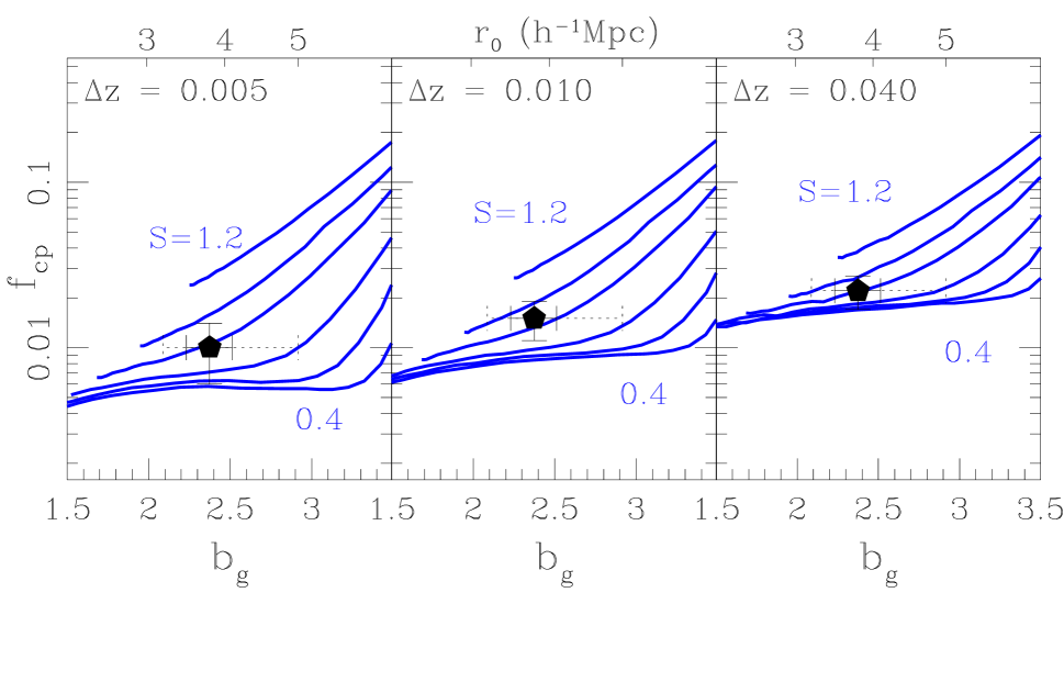
Figure 2: The fraction of pairs within an angular separation of $20^{\prime\prime}$ for three different $z$ binnings: $\Delta z=0.005,0.010,$ and $0.040$, shown as a function of the galaxy bias. The four lines in each panel correspond to halo occupation slopes of $S=1.1,1.0,0.8,0.6$ and $0.4$. The number density of galaxies is fixed to the observed value for spectroscopically-confirmed LBGs. The sharp upturn in the $S=0.4$ line occurs at a bias of $\sim 3.2$, which is the maximum bias for an $S=0.0$ model ($p=1.0$). In order to obtain a bias greater than this for the $S=0.4$ case, ${M}_{\rm min}$ must be larger than ${M}_{1}$, which forces all haloes to host more than one galaxy on average, and thus increases the close pair fraction drastically. The data points and solid-line error bars show determinations of $f_{cp}$ and $b_{g}$ from the A01 and Adelberger (2000) samples respectively. The dotted-line error bars reflect the range in $b_{g}$ determinations from a number of recent estimates (see text), providing a reasonable estimate of the systematic uncertainty in determining $b_{g}$.

The thin vertical line corresponds to an $S=0.0$ model with $p=1.0$. This corresponds to the simple ‘one-galaxy-per-massive-halo’ type model that has often been considered in previous works. As we discussed in Section 2, for the special case $S=0$, ${M}_{1}$ is irrelevant and we must assign a value for the selection probability $p$ in order to obtain a value for ${M}_{\rm min}$ that provides the desired (observed) density $n_{g}$. Since $p$ cannot exceed $1.0$, this vertical line represents an upper limit on the value of ${M}_{\rm min}$ for a given value of $n_{g}$. Note that for this reason, it is possible to find combinations of $n_{g}$ and $b_{g}$ that cannot be reproduced simultaneously in this sort of model (ie. if $n_{g}$ is ‘too high’ for the given bias value). Similarly, as $p$ is lowered in an $S=0.0$ model, subject to the constraint that the observed value of $n_{g}$ is fixed, the implied ‘true’ number density increases, and ${M}_{\rm min}$ must be reduced accordingly. Since low-mass haloes are less strongly clustered, the corresponding predicted bias will also decrease. The (dashed) lines of constant bias in Fig. 1 approach vertical asymptotes at the value of ${M}_{\rm min}$ that produces this bias in the $S=0.0$ case. For example, if $S=0.0$ and $p=0.1$, then the observed number density requires ${M}_{\rm min}\simeq 1.2\times 10^{11}{h^{-1}}{\rm M}_{{}_{\mathord{\odot}}\;}$ and gives $b_{g}\simeq 2.2$. Note that the $b_{g}=2.2$ dashed line approaches its vertical asymptote at the same value of ${M}_{\rm min}$.

Even if only the number density and large-scale bias are known, Fig. 1 already places strong limits on the halo occupation function for $z\sim 3$ galaxies. For example if the observed LBG bias is constrained at $b_{g}<3$, then the critical mass above which halos host more than one observed galaxy at $z\sim 3$ must be rather large, ${M}_{1}\ga 4\times 10^{12}{h^{-1}}{\rm M}_{{}_{\mathord{\odot}}\;}$, regardless of the values of $S$ and ${M}_{\rm min}$. If $b_{g}$ is estimated to lie within some well-defined range, then, independent of the the occupation function slope $S$, the model parameters ${M}_{1}$ and ${M}_{\rm min}$ must lie in a region defined by the two (dashed) bias lines corresponding to that range. For example, the bias estimate from Adelberger (2000) is $b_{g}\simeq 2.2-2.5$. The allowed region implied by this measurement is indicated by the shaded band in Fig. 1. Specifically, for ${M}_{1}\ga 5\times 10^{13}{h^{-1}}{\rm M}_{{}_{\mathord{\odot}}\;}$ this implies ${M}_{\rm min}\simeq(1-2)\times 10^{11}{h^{-1}}{\rm M}_{{}_{\mathord{\odot}}\;}$, and for ${M}_{\rm min}\la 10^{11}{h^{-1}}{\rm M}_{{}_{\mathord{\odot}}\;}$ (and $S>0$), it implies ${M}_{1}\simeq(5-50)\times 10^{12}{h^{-1}}{\rm M}_{{}_{\mathord{\odot}}\;}$.

In Fig. 2, we have again fixed the number density to match the observed value, but now we plot the model predictions in the plane of close pair fraction versus the large-scale bias (note that both quantities are directly observable). Recall that in estimating $f_{cp}$, we use angular bins of radius $20^{\prime\prime}$ ($0.4$ comoving ${h^{-1}}$Mpc  at $z=3$ in our adopted cosmology). The pairs are defined in redshift bins of $\Delta z=0.005,0.010,$ and $0.040$, as indicated separately in each panel. The solid lines show model predictions for fixed values of the slope, $S=1.1,1.0,0.8,0.6,$ and $0.4$. The high-$S$ lines lie above those of lower $S$. The lines are truncated at a bias corresponding to ${M}_{\rm min}=10^{8}{h^{-1}}{\rm M}_{{}_{\mathord{\odot}}\;}$. This is an extremely conservative lower limit on the expected mass of halos that can host LBGs — two orders of magnitudes smaller than lower limit on the LBG host mass derived by Pettini et al. (2001) using equivalent widths of nebular emission lines.

The curves tend to be flatter at low bias and to rise more steeply at large bias. This corresponds to a transition between a close pair density that is dominated by projection ($n_{\rm cp}^{\rm d}$) at low bias, and is dominated by objects within the same halo ($n_{\rm cp}^{\rm h}$) at high bias (see Eq. 9). As the close pair fraction is calculated for larger and larger bins in redshift $\Delta z$, the contribution due to galaxies in projection becomes larger, while that coming from objects within the same halo remains the same. This is why, for low-$b_{g}$, the values of $f_{cp}$ generally change from one panel to the next, while for high-$b_{g}$ there is very little change. This tendency also provides an additional constraint. In principle the model can be constrained with one choice of $\Delta z$, but by looking at data with various choices of the redshift bin, we can get an additional handle on the fraction of the close pairs coming from same-halo galaxies and from projection effects. For example, a strong change in close pair fraction with $z$ binning would indicate that the close pairs are dominated by projection effects.

The behavior at high bias, corresponding to the single-halo dominated regime, can be understood by examining Fig. 1. For a fixed slope, the typical number of objects within the same halo depends primarily on the value of ${M}_{1}$ relative to ${M}_{\rm min}$. Since ${M}_{1}$ is the mass above which haloes typically host more than one galaxy, if ${M}_{1}$ is much larger than ${M}_{\rm min}$, then most haloes will have fewer than one object, and the close pair fraction will be small. Similarly, if ${M}_{1}\simeq{M}_{\rm min}$ then a large fraction of haloes will host multiple galaxies, and the close pair fraction is high. The slopes of the $f_{\rm cp}-b_{g}$ relation are steeper for low-$S$ models because the ${M}_{1}-{M}_{\rm min}$ relation is also steeper for these models. The transition from projection-dominated to same-halo-dominated occurs at larger bias for lower $S$ models for the same reason. In contrast to the single-halo piece, the projection-dominated (low-bias) regime tends to be steeper for high-$S$ models. The reason again is associated with the slopes of the ${M}_{1}-{M}_{\rm min}$ curves shown in Fig. 1. The projected close pair density, $n_{\rm cp}^{\rm d}$, (Eq. 12) is proportional to the amplitude of the distinct halo correlation function. Therefore one might expect that $n_{\rm cp}^{\rm d}$ simply would grow as a function of bias, and indeed it does for high-$S$ models. The reason why the low-$S$ models show very little change as a function of bias is that this tendency is compensated by the rapid change in ${M}_{\rm min}$ as a function of bias in these models. As ${M}_{\rm min}$ increases, so does the typical halo size, and therefore the region over which the halo-exclusion drives the separate halo correlation function to zero becomes larger. For $S=0.4$, the typical halo exclusion size grows so rapidly with the bias that it cancels out the effect of increasing the correlation function amplitude at large scales. (The $S=0$ case looks nearly identical to the $S=0.4$ out to a bias of about $3.2$, which is why we do not plot any smaller values of $S$).

The data points on Fig. 2 show the estimates of close pair fraction and $1-\sigma$ uncertainties derived from the A01 data set, as discussed in Section 2, along with the bias value and its statistical $1-\sigma$ uncertainty from Adelberger (2000). We use the bias and error from Adelberger (2000) because this sample is very similar to that of A01. However, the formal uncertainty quoted for this value likely underestimates the precision to which we know the value of $b_{g}$, since best estimates tend to vary for different samples and methods (see Table 1). In order to allow for this, we show a dotted error bar, which spans the range of recent determinations ($b_{g}=2.1-2.9$). From now on, we refer to the Adelberger (2000) uncertainty (solid line error bar) as our fiducial bias range and the larger uncertainty (dotted line error bar) as our our expanded range.

The data seem to favor a model with $S\simeq 1.0$. The fact that this slope seems to reproduce the observed $f_{cp}$ counts (within fiducial errors) for all three $\Delta z$ binnings is encouraging, and is also an indication that our simplified halo occupation model provides a reasonable description of the galaxy-to-halo relation for this sample. The $\Delta z=0.01$ panel provides the strongest constraint, and within the fiducial $1-\sigma$ uncertainties shown, the compatible range of model slopes is $S\simeq 0.9-1.1$, with larger values of bias preferring shallower slopes. The expanded bias range is consistent with a slightly larger slope range $S\simeq 0.8-1.1$.

Fig.  3 maps the constraints shown in Fig. 2 to the allowed regions in ${M}_{1}$ and ${M}_{\rm min}$ parameter space. Allowed regions are filled with closely spaced slanted lines. For each observationally-consistent value of $b_{g}$, there is a range of $S$ values that are allowed by the close pair constraint. Correspondingly, there are well-defined regions in ${M}_{1}$ and ${M}_{\rm min}$ space consistent with each $S$ and $b_{g}$ combination, as indicated by the slanted line-filled bands. It is important to realize that each point in a filled region represents a unique model combination of $S$, ${M}_{1}$, and ${M}_{\rm min}$. The solid lines, representing models of constant $S$ in this space, are shown to help guide this understanding.

The left panel shows the region consistent with our fiducial bias range and the right panel corresponds to the expanded bias range. No strong statistical significance should be attached to the filled bands — they simply represent areas in parameter space that provide overlap between the theoretical predictions and the data shown in Fig. 2. We have neglected any error in the analytic estimates, which is likely of the order of $\sim 10$ per cent in $f_{cp}$ and $b_{g}$. The main point to take away is that the allowed parameter space has been significantly reduced compared to that shown in Fig. 1. For our fiducial bias uncertainty we find that ${M}_{\rm min}$ should lie roughly in the range $(0.4-8)\times 10^{10}{h^{-1}}{\rm M}_{{}_{\mathord{\odot}}\;}$ and ${M}_{1}\simeq(6-10)\times 10^{12}{h^{-1}}{\rm M}_{{}_{\mathord{\odot}}\;}$. For the expanded uncertainty range, the allowed space for ${M}_{\rm min}$ expands as well, ${M}_{\rm min}\simeq(0.1-20)\times 10^{10}{h^{-1}}{\rm M}_{{}_{\mathord{\odot}}\;}$, but the ${M}_{1}$ range remains roughly the same. Note that larger allowed values for ${M}_{\rm min}$ correspond to lower values of $S$ (at fixed $f_{cp}$).

Figure 3: Allowed region of halo occupation function parameter space implied by all three observational constraints ($n_{g}$, $f_{cp}$ and $b_{g}$), with and without scatter in the halo occupation statistics. Solid lines show models of constant slope $S$. (Left) Filled regions indicate the parameter space consistent with $1-\sigma$ bias errors from Adelberger (2000). (Right) Filled regions show how the allowed model space expands when a larger range for the bias is allowed (see text).

It is useful at this point to explore how an intrinsic scatter in halo occupation would affect these estimates of the allowed model parameter space. Until this point, we have assumed a deterministic relation between a halo’s mass and the number of galaxies it hosts, but any realistic model of galaxy formation will surely predict at least some scatter in this quantity. In principle, this distribution about the mass-occupation relation could be treated as an additional input of the model, however, here we will work out a simple case motivated by semi-analytic galaxy formation scenarios in order to illustrate how scatter affects our results.

Scatter in the halo occupation function will have no effect on the predictions of number density and large-scale bias, and will alter only the close pair fraction associated with same-halo pairs. In order to account for these, we must alter Eq. 13 by replacing ${N}_{g}({N}_{g}-1)$ with the appropriate expression for $\left<{N}_{g}({N}_{g}-1)\right>$. Although one might suppose that a Poisson distribution would be a reasonable assumption, $\left<{N}_{g}({N}_{g}-1)\right>={N}_{g}^{2}(M)$, such an assumption is physically unrealistic for $N_{g}\la 1$, or $M\la{M}_{1}$. As the host mass falls below that typical for containing an object, the likelihood for it to host any additional objects becomes suppressed simply by mass counting arguments. This kind of sub-Poisson scatter is seen for low-mass hosts in semi-analytic models of galaxy formation (e.g. Scoccimarro et al., 2001). For our illustrative example, we will use the same halo pair counting observed in the semi-analytic models presented in W01 and Somerville et al. (2001a), which becomes sub-Poisson below ${N}_{g}\sim 1$:

$$\left<N_{g}(N_{g}-1)\right>=\left\{\begin{array}[]{cc}N_{g}^{2}&\mbox{ ${N}_{g}\geq 1$}\\ N_{g}^{2}\ln(4N_{g})/\ln(4)&\mbox{$0.25<{N}_{g}<1$}\\ 0&\mbox{ ${N}_{g}\leq 0.25$}\end{array}\right.$$ (17)

We have suppressed the implicit mass dependence in ${N}_{g}\equiv{N}_{g}(M)$. Although the Somerville et al. (2001a) models are best described by an occupation function with $S\sim 0.7-0.8$, we assume here that the above formula holds for all values of $S$.

The results of this calculation are shown in Fig. 4. When the average number of objects is small, including scatter increases the probability of having multiple objects in the same halo, and consequently increases the expected close pair count. For this reason, the steeply rising portions of the $f_{cp}-b_{g}$ curves begin to become important at lower values of $b_{g}$ relative to those in Fig. 2. It is encouraging that even with the inclusion of this substantial amount of scatter, the data appear to favor a slope similar to that suggested by the zero-scatter models shown in Fig. 2, although slightly lower, $S\simeq 0.9$. The fiducial $1-\sigma$ errors overlap with the model curves for $0.7\la S\la 1.0$, and the expanded bias uncertainty extends the allowed range to somewhat shallower slopes, $0.4\la S\la 1.0$. The corresponding allowed regions in ${M}_{1}$-${M}_{\rm min}$ space for the fiducial (left panel) and expanded (right panel) bias ranges are indicated by the vertically-shaded bands in Fig. 3. The ranges of preferred ${M}_{\rm min}$ values have significant overlap with those in the zero-scatter case: ${M}_{\rm min}\simeq(1-13)\times 10^{10}{h^{-1}}{\rm M}_{{}_{\mathord{\odot}}\;}$ for fiducial bias uncertainty, and ${M}_{\rm min}\simeq(0.6-40)\times 10^{10}{h^{-1}}{\rm M}_{{}_{\mathord{\odot}}\;}$ for the expanded case. However, the preferred regions are offset towards higher ${M}_{1}$ by roughly a factor of two; this is due to the fact that increasing the scatter increases the close pair fraction and thus the number of objects per halo must be decreased by increasing ${M}_{1}$. Note, however, that the constraint on the minimum halo mass ${M}_{\rm min}$ is more robust to the inclusion of scatter.

Figure 4: Close pair fraction as a function of bias for different values of the halo occupation slope, as in Fig. 2, but including a non-zero scatter about the halo occupation relation, as described in the text. The number density is fixed to the observed value for the A01 sample of Lyman-break galaxies, as usual. The fraction of pairs within an angular separation of 20 arcsec is shown for three different $z$ binnings: $\Delta z=0.005,0.010,$ and $0.040$, as a function of large-scale bias. The four lines in each panel correspond to halo occupation slopes of $S=1.0,0.8,0.6,0.4,$ and $0.2$.

5 Luminosity/Number Density Dependence

So far, we have considered observational constraints for a population of galaxies with a given magnitude limit. However, it is interesting to consider how the predicted properties would change for samples with different magnitude limits. Because the observed number density is a function of the magnitude limit of the sample (for a sample of known completeness), this can also be thought of as considering different values for the observed number density.

Such a prediction is particularly relevant in light of the work by Giavalisco & Dickinson (2001, GD01), which suggests a correlation between the LBG clustering amplitude and intrinsic galaxy luminosity. GD01 compared correlation lengths obtained from ground-based spectroscopic and photometric samples, and a deeper sample of LBGs identified in the Hubble Deep Field. They found that the correlation length strongly decreased as the magnitude limit of the sample grew fainter, or, similarly, as the observed number density of the population increased. If correct, this result has interesting implications for the relationship between observed galaxies and dark haloes. Unfortunately, a prediction for the expected clustering as a function of observed number density is rather unconstrained in our model. This is because, in principle, all three of our model parameters could vary as a function of galaxy luminosity.

We can overcome this problem by making some plausible simplifying assumptions. For example, perhaps the simplest possibility is that the value of $S$ stays fixed when the number density/luminosity cutoff of a sample changes (which is roughly true in the semi-analytic models of Somerville et al. 2001b), and that ${M}_{\rm min}$ and ${M}_{1}$ vary together in the natural way ${M}_{\rm min}\propto{M}_{1}$. This assumption may be motivated qualitatively by assuming that ${M}_{\rm min}$ is proportional to the minimum observable galaxy luminosity, and that the host haloes themselves are self-similar as smaller and smaller haloes become important. For $S=0$, the ${M}_{1}$ assumption cannot apply, and is replaced by the assumption that selection probability $p$ remains fixed.

The resulting model predictions are shown in Fig. 5, for four values of the halo occupation slope $S$. We have normalized each model so that it has $b_{g}=2.4$ at the number density of the spectroscopically confirmed sample of Adelberger (2000), and predict how the bias should vary as function of $n_{g}$. The $S=0$ model shows the steepest dependence because the number density can be increased only by adding galaxies to increasingly lower mass (and less clustered) haloes.

The data points correspond to the observational estimates. The triangles show the results of GD01. The square reflects the Adelberger (2000) estimate. The angular correlation function result from recent work by Porciani & Giavalisco (2001) is shown by the pentagon. The filled circle shows the results of Arnouts et al. (1999) based on a sample from the HDF with a similar magnitude limit as the GD01 HDF data, but selected via photometric redshifts rather than the Lyman-break technique. We have not included the Adelberger et al. (1998) determination of the bias because it has been superseded by the Adelberger (2000) sample, which uses a larger sample of galaxies and the same counts-in-cells method. In light of the disagreement between the various estimates at fixed density, the strength of the trend must be regarded as rather uncertain. If the GD01 points are neglected, then all four models are consistent with the data, but taken together, the data seem to favor a model closer to the $S=0.0$ line, unlike the close-pair and bias constraints discussed in the previous sections, which favored $S\sim 0.9-1.0$.

However, it is important to note that the GD01 points cannot be reproduced by any of these minimum-assumption models, as even the $S=0.0$ model trend is too shallow. The only way to obtain such a trend would be to assume that LBGs tend to avoid the most massive haloes, corresponding to a negative slope $S$. Otherwise a trend between clustering and number density as steep that indicated by GD01 can only be accounted for by breaking one of our simplifying assumptions. For example, if the selection probability, $p$, varies systematically with the observed number density, then the low bias of the higher density sample might indicate that the true number density is simply much larger than that observed. We find that only if the selection probability varies inversely with the observed number density: $p\propto n_{g}^{-1}$ (with $p\leq 1$), can we reproduce a trend this steep with $S=0$. Although one might expect the selection probability to be higher for brighter objects, such a strong trend seems problematic for other reasons. Recall that the value of $p$ can only effect the estimate of the number density, not the bias, so this would imply that there is almost no difference in the number density of LBGs at ${\mathcal{R}}=25$ and ${\mathcal{R}\sim 27}$, which is at odds with observational determination of the luminosity function of LBGs over this range (Steidel et al., 1999).

6 Conclusions

                                                                

Figure 5: Bias (left axis), and correlation length (right axis) as a function of comoving number density, for various values of the slope. The data points are described in the text. Note that the points at high and low number density have been offset slightly in the horizontal direction in order to allow their error bars to remain distinct.

We have presented a simple and intuitive method for constraining the relationship between observed galaxies and their dark matter haloes, and used it to constrain the galaxy-halo occupation relation at $z\sim 3$. Using a three-parameter model of the form $N_{g}(M)=(M/{M}_{1})^{S}$, $M>{M}_{\rm min}$ to describe the number of observed galaxies as a function the host halo mass, we derived predictions for three observables: the galaxy number density, $n_{g}$, large-scale bias, $b_{g}$, and the fraction of galaxies in close pairs, $f_{cp}$. Given these three observed galaxy properties, the three unknown model parameters can be constrained.

We presented estimates of the allowed range for these three parameters based on the properties of galaxies in a sample of spectroscopically confirmed LBGs (Adelberger, 2000, 2001). The results are summarized in Fig. 3. For a model with no scatter about the halo occupation relation, the favored values of the slope lie in the range $0.9\la S\la 1.1$, with preferred characteristic halo masses ${M}_{\rm min}\simeq(0.4-8)\times 10^{10}{h^{-1}}{\rm M}_{{}_{\mathord{\odot}}\;}$ and ${M}_{1}\simeq(6-10)\times 10^{12}{h^{-1}}{\rm M}_{{}_{\mathord{\odot}}\;}$. For a model where the halo occupation function scatter is estimated based on semi-analytic models, the range of preferred model parameters shifts to $0.7\la S\la 1.0$, ${M}_{\rm min}\simeq(1-13)\times 10^{10}{h^{-1}}{\rm M}_{{}_{\mathord{\odot}}\;}$ and ${M}_{1}\simeq(8-15)\times 10^{12}{h^{-1}}{\rm M}_{{}_{\mathord{\odot}}\;}$. Since the observational uncertainty in $b_{g}$ is likely significantly larger than the formal error derived for the sample of LBGs we consider, we have also explored a range of biases consistent with all of the recent estimates for LBG clustering. Using this expanded range of uncertainties, we obtain $0.8\la S\la 1.1$ and ${M}_{\rm min}\simeq(0.01-20)\times 10^{10}{h^{-1}}{\rm M}_{{}_{\mathord{\odot}}\;}$ for the case of no scatter, and $0.4\la S\la 1.0$, ${M}_{\rm min}\simeq(0.6-40)\times 10^{10}{h^{-1}}{\rm M}_{{}_{\mathord{\odot}}\;}$ if scatter is included. Preferred values of ${M}_{1}$ are relatively insensitive to increasing the uncertainty in $b_{g}$, and preferred values of ${M}_{\rm min}$ are relatively insensitive to the inclusion of scatter in the occupation function.

It is interesting that the data favor a model in which the minimum halo mass for hosting an observable object, ${M}_{\rm min}$, is significantly smaller (by roughly two orders of magnitude) than the mass range above which haloes typically host more than one observed object, ${M}_{1}$. However, recall that the average mass halo hosting an observable object is typically lower: ${M}_{1}^{i}=p^{1/S}{{M}_{1}}$, so the difference between ${M}_{\rm min}$ and ${M}_{1}^{i}$ ranges from about two orders of magnitude for high $S$ values to no difference for $S=0$. In any case, this implies that most haloes hosting LBGs do not contain more than one observable object. However, as we have seen, because the most massive haloes are also the most clustered, the clustering predictions are quite sensitive to the treatment of occupation statistics in these haloes even though they constitute a small fraction by number. In addition, it is interesting that the range of allowed values for ${M}_{\rm min}$ have considerable overlap with mass estimates based on the widths of nebular emission lines, $\sim 10^{10}{h^{-1}}{\rm M}_{{}_{\mathord{\odot}}\;}$ (Pettini et al., 2001), bearing in mind that these line-widths may yield underestimates of the true virial masses. Line-width analyses such as this may provide useful additional constraints for the type of model presented here. For example, one might be inclined to eliminate models with ${M}_{\rm min}\la 10^{10}{h^{-1}}{\rm M}_{{}_{\mathord{\odot}}\;}$ based on the Pettini et al. (2001) analysis, and thus significantly reduce the allowed model parameter space. However, these line widths estimates are based on a relatively small sample of very bright objects, so placing strict limits on ${M}_{\rm min}$, which is generally much smaller than than a ‘typical’ LBG host, ${M}_{1}$, may not be justified.

Although the current level of observational uncertainty prevents us from precisely defining a favored model, the identification of an allowed range of parameter space already provides useful constraints on more sophisticated modelling aimed at understanding halo occupation at a more basic level. For example, as mentioned in the introduction, the first, and, for some, still the favored model for LBG occupation is one in which there is one galaxy per halo, $S=0.0$ (e.g. Wechsler et al., 1998). Our results disfavor such a model because it under-predicts the close pair counts (see also W01). Similarly, naive models for collision-driven LBGs (Kolatt et al., 1999) predicted a steep halo occupation function, $S\simeq 1.1$, which is the steepest slope consistent with our results and requires that LBGs populate a fraction of very low-mass halos (although in W01 we explain why the more sophisticated treatment of collisional bursts presented in Somerville et al. (2001b) yields a shallower relation, $S\sim 0.7$). The preferred range of slopes from our analysis including scatter is in agreement with the range of slopes from semi-analytic estimates for the occupation function for a range of star formation models (W01), including those in which the primary mode of star formation is merger-driven starbursts, and also those in which quiescent star formation dominates. However, it seems unlikely that the slope will be constrained well enough in the near future to distinguish between the different semi-analytic models compared in W01. Work by Porciani & Giavalisco (2001) using a counts-in-cells analysis of the angular correlation function of LBGs (using an overlapping but different sample of galaxies than considered here) favors a model with a shallower slope; their analysis is consistent with S=0. Some of the discrepancy may result from the more highly biased sample they consider. (The full A01 sample includes new fields that are less clustered than the first few fields studied). As illustrated in Fig. 2, for a fixed $f_{cp}$, a higher bias favors a shallower slope. Nonetheless, neither our constraints or theirs are very strong, and we emphasize as they do that current samples may not yet be a fair representation of the high-redshift galaxy population. When the sample becomes larger, these complementary types of analyses should be applied in parallel to constrain the halo occupation function.

We then applied this simple model to investigate how the clustering of a population of galaxies might change as a function of their observed number density, or, implicitly, as a function of their intrinsic luminosity. Under the simplest assumptions for how model parameters should vary as a function of luminosity cut, the low-$S$ models vary more strongly with number density than do high-$S$ models. None of the models are steep enough to match the trend found by GD01, but models with $S=0.0-1.0$ are consistent with the change in bias between the sample of Adelberger (2000) and Arnouts et al. (1999) — so this data cannot yet provide significant constraints. More data which can provide smaller error bars on observational parameters, especially the bias, could prove a valuable constraint for the halo occupation relation. We have shown how combinations of our three model parameters are currently constrained by the data, but with the current data sample individual parameters (such as the slope S or the minimum mass for hosting a halo ${M}_{\rm min}$) are not well determined. This will probably await a significantly larger survey, such as one that could be completed using, e.g., the Very Large Telescope (VLT) or the Large Binocular Telescope (LBT).

We have discussed here how the formalism presented in §3 can be applied to determine the halo occupation of a specific population of LBGs at $z\sim 3$, but in fact it is quite general, and could be applied to constrain the halo occupation models for a variety of galaxy populations, and used to understand the relation between various galaxy populations. The limitation of this method is that, as we have shown, it requires a large sample to be able to put strong constraints on model parameters. Moreover, the method relies on the simplifying assumption of scale-independent bias, and in cases where the slope of the galaxy correlation function is significantly different from that of the dark matter, it becomes ill-defined. However, with new generations of telescopes, large samples will become available for an increasing number of types of high redshift galaxies. Once statistics become available from the LALA survey (Rhoads et al., 2000), a similar approach to the one we have presented could be used to understand whether Lyman-$\alpha$ emitters and LBGs populate the same dark haloes, or to relate the LBG population to that of SCUBA sources — such an analysis would be complementary to the analysis of Shu, Mao & Mo (2001) which uses star formation rates and the observed size distribution to constrain halo occupation models. Similar methods can also be used to relate the LBG population at $z=3$ with galaxy populations at different redshifts (Moustakas & Somerville, in preparation). This basic formalism could also easily be applied to quasars identified in the Sloan Digital Sky Survey, as a tool for understanding the halo occupation of quasars as a function of redshift and luminosity.

References

- Adelberger (2000) Adelberger K. L., 2000, in Mazure A., Le Fevre O., Le Brun V., eds, Clustering at High Redshift Vol. 200 of ASP Conference Series, Star formation and structure formation at . Kluwer Academic Publishers, p. 13
- Adelberger (2001) Adelberger K. L., 2001, PhD thesis, California Institute of Technology
- Adelberger et al. (1998) Adelberger K. L., Steidel C. C., Giavalisco M., Dickinson M., Pettini M., Kellogg M., 1998, ApJ, 505, 18
- Arnouts et al. (1999) Arnouts S., Cristiani S., Moscardini L., Matarrese S., Lucchin F., Fontana A., Giallongo E., 1999, MNRAS, 310, 540
- Bagla (1998) Bagla J. S., 1998, MNRAS, 297, 251
- Benson (2001) Benson A. J., 2001, preprint, astro-ph/0101278
- Benson et al. (2000) Benson A. J., Cole S., Frenk C. S., Baugh C. M., Lacey C. G., 2000, MNRAS, 311, 793
- Berlind & Weinberg (2001) Berlind A., Weinberg D. H., 2001, in preparation
- Bullock et al. (2001) Bullock J. S., Kolatt T. S., Sigad Y., Somerville R. S., Kravtsov A. V., Klypin A. A., Primack J. R., Dekel A., 2001, MNRAS, 321, 559
- Bullock et al. (1999) Bullock J. S., Kolatt T. S., Somerville R. S., Sigad Y., Kravtsov A. V., Klypin A. A., Primack J. R., Dekel A., 1999, in Holt S., Smith. E., eds, After the Dark Ages: When Galaxies were Young. 9th Annual October Astrophysics Conference in Maryland held 12-14 October, 1998. College Park, Maryland. Lyman break galaxies as collision-driven starbursts. American Institute of Physics Press, p. 216
- Coles et al. (1998) Coles P., Lucchin F., Matarrese S., Moscardini L., 1998, MNRAS, 300, 183
- Cooray (2001) Cooray A., 2001, PhD thesis, University of Chicago
- Dekel & Lahav (1999) Dekel A., Lahav O., 1999, ApJ, 520, 24
- Giavalisco & Dickinson (2001) Giavalisco M., Dickinson M. E., 2001, ApJ, 550, 177
- Giavalisco et al. (1998) Giavalisco M., Steidel C. C., Adelberger K. L., Dickinson M. E., Pettini M., Kellogg M., 1998, ApJ, 503, 543
- Jenkins et al. (2001) Jenkins A., Frenk C. S., White S. D. M., Colberg J. M., Cole S., Evrard A. E., Couchman H. M. P., Yoshida N., 2001, MNRAS, 321, 372
- Jing et al. (1998) Jing Y. P., Mo H. J., Boerner G., 1998, ApJ, 494, 1
- Jing & Suto (1998) Jing Y. P., Suto Y., 1998, ApJ, 494, L5
- Klypin et al. (1999) Klypin A., Gottlöber S., Kravtsov A. V., Khokhlov A. M., 1999, ApJ, 516, 530
- Kolatt et al. (1999) Kolatt T. S., Bullock J. S., Somerville R. S., Sigad Y., Jonsson P., Kravtsov A. V., Klypin A. A., Primack J. R., Faber S. M., Dekel A., 1999, ApJ, 523, L109
- Mo & Fukugita (1996) Mo H. J., Fukugita M., 1996, ApJ, 467, L9
- Moore et al. (1999) Moore B., Ghigna S., Governato F., Lake G., Quinn T., Stadel J., Tozzi P., 1999, ApJ, 524, L19
- Moscardini et al. (1998) Moscardini L., Coles P., Lucchin F., Matarrese S., 1998, MNRAS, 299, 95
- Peacock & Smith (2000) Peacock J. A., Smith R. E., 2000, MNRAS, 318, 1144
- Pettini et al. (2001) Pettini M., Shapley A. E., Steidel C. C., Cuby J.-C., Dickinson M., Moorwood A. M. F., Adelberger K. L., Giavalisco M., 2001, ApJ, in press
- Porciani & Giavalisco (2001) Porciani C., Giavalisco M., 2001, ApJ, submitted
- Rhoads et al. (2000) Rhoads J. E., Malhotra S., Dey A., Stern D., Spinrad H., Jannuzi B. T., 2000, ApJ, 545, L85
- Scoccimarro et al. (2001) Scoccimarro R., Sheth R. K., Hui L., Jain B., 2001, ApJ, 546, 20
- Seljak (2000) Seljak U., 2000, MNRAS, 318, 203
- Sheth et al. (2001) Sheth R. K., Mo H. J., Tormen G., 2001, MNRAS, 323, 1
- Sheth & Tormen (1999) Sheth R. K., Tormen G., 1999, MNRAS, 308, 119
- Shu et al. (2001) Shu C., Mao S., Mo H. J., 2001, preprint, astro-ph/0102456
- Sigad et al. (2000) Sigad Y., Kolatt T., Bullock J., Kravtsov A. V., Klypin A. A., Primack J. R., Dekel A., 2000, preprint, astro-ph/0005323
- Somerville et al. (2001) Somerville R. S., Lemson G., Sigad Y., Dekel A., Kauffmann G., White S., 2001, MNRAS, 320, 289
- Somerville & Primack (1999) Somerville R. S., Primack J. R., 1999, MNRAS, 310, 1087
- Somerville et al. (2001a) Somerville R. S., Primack J. R., Faber S. M., 2001a, MNRAS, 320, 504
- Somerville et al. (2001b) Somerville R. S., Primack J. R., Faber S. M., 2001b, MNRAS, 320, 504
- Springel (1999) Springel V., 1999, PhD thesis, , Ludwig-Maximilians-Univ., (1999)
- Steidel et al. (1998) Steidel C. C., Adelberger K. L., Dickinson M., Giavalisco M., Pettini M., Kellogg M., 1998, ApJ, 492, 428
- Steidel et al. (1999) Steidel C. C., Adelberger K. L., Giavalisco M., Dickinson M., Pettini M., 1999, ApJ, 519, 1
- Wechsler (2001) Wechsler R. H., 2001, PhD thesis, University of California, Santa Cruz
- Wechsler et al. (2000) Wechsler R. H., Bullock J. S., Somerville R. S., Kolatt T. S., Primack J. R., Blumenthal G. R., Dekel A., 2000, in Mazure A., Le Févre O., Le Brun V., eds, ASP Conference Series 200: Clustering at High Redshift Clustering of high-redshift galaxies: Relating lbgs to dark matter halos. p. 29
- Wechsler et al. (1998) Wechsler R. H., Gross M. A. K., Primack J. R., Blumenthal G. R., Dekel A., 1998, ApJ, 506, 19
- Wechsler et al. (2001) Wechsler R. H., Somerville R. S., Bullock J. S., Kolatt T. S., Primack J. R., Blumenthal G. R., Dekel A., 2001, ApJ, 554, 1