The effects of relativistic bulk motion of X-ray flares in the corona on the iron K$\alpha$ line in Seyfert 1 galaxies

Abstract

It is likely that dramatic magnetic flares in a corona above a black hole accretion disk dominate the X-ray emission in Seyfert 1 galaxies. Such flares are likely to move with mildly relativistic bulk velocity. We study the effects of the bulk motion of X-ray flares on the shape and equivalent width of the iron K$\alpha$ line from an untruncated cold disk around a Kerr black hole using fully relativistic calculations. The flares are located above a cold accretion disk$-$either on or off the rotation axis. The upward/outward bulk motion of flares causes a reduction of the iron K$\alpha$ line width, while the downward/inward bulk motion of flares causes an increase of the iron K$\alpha$ line width. To a distant observer with a low inclination angle ($\theta_{\rm o}\lower 1.93747pt\hbox{$\;\buildrel<\over{\sim}\;$}30\arcdeg$), larger upward/outward bulk velocities decrease the extension of the red wing, with little change in the location of the blue ‘edge’. In contrast, an observer at a large inclination angle (e.g. $\theta_{\rm o}=60\arcdeg$) sees both the red wing and the blue ‘edge’ change with the bulk velocity. The equivalent width of the iron K$\alpha$ line decreases rapidly with increasing bulk velocity of flares. However, the ‘narrower’ line profiles observed in some objects (e.g. IC4329A and NGC4593) are difficult to produce using the out-flowing magnetic flare model with an appropriate equivalent width unless the X-ray emission is concentrated in an outer region with a radius of several tens of $r_{\rm g}=GM/c^{2}$ or more. This suggests that other parameters, such as the ‘truncation radius’ due to disruption or ionization of the inner disk may still be needed. An important result is that the iron K$\alpha$ line intensity is found to be constant even though the continuum flux varies significantly, which is true for out-flowing magnetic flares with different bulk velocities but similar intrinsic luminosities when located close to the central black hole. This is caused by the combination of the effects of relativistic beaming and gravitational lensing. We find that fluctuations in the bulk velocities of out-flowing low-height flares located at the inner region ($r\lower 1.93747pt\hbox{$\;\buildrel<\over{\sim}\;$}15r_{\rm g}$) can account for a constant iron K$\alpha$ line and significant continuum variation as observered in MCG-6-30-15 and NGC5548. This is especially interesting for MCG-6-30-15 whose behavior is difficult to explain using the ionization model.

1 Introduction

Two prominent X-ray features, the iron K$\alpha$ line at 6.4 keV and the broad Compton reflection hump, have been found in Active Galactic Nuclei (AGNs) and in galactic black hole candidates (GBHCs) using observations made with the Ginga, ASCA, RXTE, and BeppoSAX satellites. These features have been explained as the Compton re-processing imprints of the hard X-ray power-law continuum impinging on the surface layer of a thin accretion disk (George & Fabian, 1991; Matt, Perola & Piro, 1991, and references therein). The iron K$\alpha$ line is thought to be produced by the fluorescence of the cold disk material and is accompanied by the Compton-scattered continuum.

The iron K$\alpha$ line was first observed by Ginga (e.g. Pounds et al. 1990; Nandra & Pounds 1994). The observations from ASCA have since confirmed that the line profile is both very broad and skewed (Tanaka et al., 1995; Nandra et al., 1997); these properties are generally believed to be caused by both special relativistic (i.e. transverse-Doppler and special relativistic boosting) and general relativistic (i.e. gravitational redshifts and light bending) effects. (Fabian et al., 1989; Laor, 1991; Kojima, 1991). In MCG-6-30-15, the line profiles provide evidence of line emission from the region very close to the central black hole, at a radius less than $5r_{\rm g}$ (where $r_{\rm g}=GM/c^{2}$ is the gravitational radius, $G$ is the gravitational constant; and $c$ is the speed of light; hereafter $G=c=1$ and thus $r_{\rm g}=M$) (Iwasawa et al., 1996, 1999). So far, alternative models have failed to consistently interpret the broad iron K$\alpha$ line profile and the continuum spectrum (Fabian et al., 1995, 2000).

There are two main aspects of the theoretical work on the broad iron K$\alpha$ line. One aspect is to study the detailed properties of the “reflector”, i.e. the accretion disk. Considering the geometry, size and ionization state of the accretion disk, reflection spectra have been computed by performing simulations of Compton reflection from neutral or ionized matter, including fluorescent iron emission (George & Fabian, 1991; Matt, Perola & Piro, 1991; Matt et al., 1992; Życki & Czerny, 1994; Matt, Fabian & Ross, 1993, 1996; Ross, Fabian & Brandt, 1996; Ross, Fabian & Young, 1999; Nayakshin, Kazanas & Kallman, 2000). The finite thickness, radial accretion flow, turbulence (Pariev & Bromley, 1998) and warp of the disk (Hartnoll & Blackman, 2000) have also been considered and shown to significantly affect the line emission. The second aspect is the study of the effects of primary X-ray emission sources (which provide energetic X-ray photons to illuminate the accretion disk) on the line properties. Dramatic magnetic flares probably dominate the X-ray emission in AGNs, and the general axisymmetric emissivity law is therefore not realistic for a time-dependent study due to the arbitrary location of X-ray flares (though it may be appropriate for some time-averaged studies). Some simple models have shown that the line profile and equivalent width (EW) change significantly with the location of the flares (Reynolds et al., 1999; Yu & Lu, 2000; Ruszkowski, 2000; Dabrowski & Lasenby, 2001). In this paper, we follow the second aspect and study the effects of the bulk motion of X-ray emitting flares on the iron K$\alpha$ line properties.

The reflection fraction $R=\Omega/2\pi$, where $\Omega$ is the solid angle subtended by the reflecting material, was found to be in the range $0-1$ or even $>1$ in some objects observed by Ginga and BeppoSAX (Pounds et al., 1990; Nandra & Pounds, 1994; Matt, 2000). The average reflection fraction is around $0.5$. An interesting correlation between the reflection fraction $R$ and the photon index $\Gamma$ for both AGNs and GBHCs has been claimed by Zdziarski, Lubi$\acute{\rm n}$ski & Smith (2000). On average, sources with flat (i.e. smaller photon index) continuum spectra tend to have a low reflection fraction. This relation is interpreted as follows: The cold (neutral or weakly ionized) thin disk extends down to only several tens of $M$, and within this radius is either disrupted (Esin, McClintock & Narayan, 1997; Poutanen, Krolik & Ryde, 1997) or totally ionized (Ross, Fabian & Young, 1999; Nayakshin, Kazanas & Kallman, 2000); this leads to a reflection fraction in the range $0-1$. An alternative model is that the reduction (or enhancement) of the reflection fraction is caused by mildly relativistic outflow (or inflow) in the corona above an untruncated accretion disk (Beloborodov, 1999b). In this model, the reflection fraction can be either $>1$ or $<1$, and a good fit of the $R-\Gamma$ relation can be obtained (Beloborodov, 1999b; Malzac, Beloborodov & Poutanen, 2001). However, one should be cautious about the $R-\Gamma$ relation since recent investigations have shown that this correlation is at least partly caused by systematic errors in data fitting (Nandra et al., 2000; Vaughan & Edelson, 2000). The extensive simulations of Vaughan & Edelson (2000) show that the correlation can result from measuring the two quantities from the same spectra. Further investigations are needed to determine whether a real correlation between $R$ and $\Gamma$ exists.

The Monte-Carlo simulations of George & Fabian (1991) have shown a relation between the reflection fraction $R$ and the EW of iron K$\alpha$ lines [EW(K$\alpha$) $\sim 130R$ eV for a typical photon index of Seyfert 1 galaxies with $\Gamma=1.90$ and for solar metallicity]. For a fixed disk/corona geometry and ionization, i.e. where $R$ is a constant, the iron K$\alpha$ line EW is expected to remain constant and the line flux increases with increasing continuum flux if the probing timescale is longer than the light crossing time of the emission-line region, which is generally true for ASCA observations of AGNs. If there is a change in the geometry of the system, the line EW is expected to vary in step with the reflection fraction $R$. From observations using ASCA, the average EW of iron K$\alpha$ lines for Seyfert 1 galaxies is about $200-300$ eV (Nandra et al., 1997), which is considerably larger than expected from the $R-$EW relation and the observed $R$ value ($R$ typically $<1$). It is difficult to understand this difference since the fluorescence must be accompanied by the Compton-scattered continuum. Recently, Lubi$\acute{\rm n}$ski & Zdziarski (2001) re-analyzed the average spectra and obtained average line profiles for three sets of Seyfert 1 galaxies grouped according to the spectral index of the X-ray continuum. Modeling the profile with a disk line plus a narrow line component, they found that the EW is consistent with $R$ following the expected relation above. However, it is still puzzling that in some bright objects the line flux appears constant (or the EW is inversely proportional to the continuum flux) and the EW is anti-correlated with $R$ while the continuum flux varies strongly. For example, the relationship between the EW and the continuum flux ($F$) in NGC5548 can be well fit by a power-law EW(K$\alpha$)$\propto F^{\alpha}$ with a slope of $\alpha=-0.9\pm 0.4$; this is consistent with a constant line flux (see Fig. 4 in Chiang et al. 2000). Similar results are observed in MCG-6-30-15 (see Table 4 and Fig. 13b in Lee et al. 2000). The reason that $R$ fails to trace the variation in the EW is still unknown. Two possible mechanisms, the thermal instability of photon-ionized plasma leading to a highly ionized skin on the surface of the thin accretion disk (Nayakshin, Kazanas & Kallman, 2000) and resonant trapping followed by Auger destruction (Ross & Fabian, 1993) may suppress the iron K$\alpha$ line emission relative to the reflection continuum (Reynolds, 2000b; Ballantyne, Ross & Fabian, 2001; Życki & R$\acute{\rm o}$ża$\acute{\rm n}$ska, 2001).

The rapid X-ray variability in many Seyfert 1 galaxies suggests that the X-ray is likely to be emitted during dramatic flare-like events (e.g. the light curve of MCG-6-30-15 in Iwasawa et al. 1999). Magnetic flares have long been considered as the source of rapid variability for accreting black holes (Galeev, Rosner & Vaiana, 1979). The variability of the X-ray source can induce the corresponding variation in the iron K$\alpha$ line. Fabian et al. (1989) suggested that any variation of the primary X-ray source would be ‘echoed’ by the evolution of the iron K$\alpha$ line profile, which was then considered in detail by Stella (1990), Matt & Perola (1992) and Campana & Stella (1993); cs95, the latter for different source geometries. Recently, Reynolds et al. (1999) generalized this work, assuming an instantaneous static X-ray flash (on- or off-axis) atop a thin disk. Their calculations of iron K$\alpha$ line reverberation show that it is possible to probe both the mass and spin of black holes in AGNs from the reverberation mapping signatures using the planned X-ray satellite Constellation X-ray Mission (Young & Reynolds, 2000).

It is likely that the dramatic magnetic flares in the inner region (e.g. $r\lower 1.93747pt\hbox{$\;\buildrel<\over{\sim}\;$}15M$) dominate the X-ray emission (Merloni & Fabian, 2001) and move with mildly relativistic bulk velocity (Reynolds & Fabian, 1997; Beloborodov, 1999a); this may play an important role in producing the reflection and the fluorescent iron line. Reynolds & Fabian (1997) estimated the special relativistic effects of the bulk motion of the X-ray emitting material (relative to the disk) on the line EW. They found that the line EW is significantly enhanced (or reduced) if the bulk motion of the X-ray source is moving directly towards (or away from) the disk, as intuitively expected. The line EW is also found to be enhanced (but to a lesser degree) if the X-ray emitting material moves along the surface of the disk. The X-ray reflection from the disk is also reduced (or enhanced) due to bulk motion of the X-ray source away from (towards) the reflector, i.e., disk, by the special relativistic beaming effect (Beloborodov, 1999b). For flares with bulk motion, the corresponding reverberation mapping properties are also expected to differ from those derived for static flares by Reynolds et al. (1999). In the present paper, we perform a complete relativistic calculation (combining both special relativistic and general relativistic effects simultaneously) to investigate the impact of the bulk motion of flares in the corona on the profile and EW of the iron K$\alpha$ line (the ionization of the reflecting material is not considered). We describe the model in §2. Calculation results are presented in §3, The discussion and applications are presented in § 4 and conclusions are given in §5.

2 Model assumptions and calculations

2.1 The X-ray flare and the disk illumination

We shall assume that the primary X-ray flares are located above the inner region of an accretion disk. In the following calculation, we assume the flare is not instantaneous flash but a constant source of illumination (i.e. not time dependent). Assuming that the flare is point-like, the X-ray photons emitted by the flare can freely propagate to the observer, the accretion disk and the black hole without absorption or attenuation. If the flaring plasma in the corona is composed of electron-positron ($e^{\pm}$) pairs, it should be accelerated away from the disk by the pressure of soft radiation which dominates the bolometric luminosity of the disk (Beloborodov, 1999a). The bulk velocity is expected to be in the range 0.1—0.7 (Beloborodov, 1999b). Field & Rogers (1993) argued that magnetic instabilities and reconnection events in a disk/corona could produce shock waves and/or streaming of relativistic particles along the magnetic field lines, similar to the ejection in solar flares; the corresponding X-ray emitting plasma may therefore be in bulk motion relative to the disk. The plasma can be ejected away or towards the disk, with the preferential direction being away from the disk (Beloborodov, 1999c). It is then reasonable to assume that the flare moves with mildly relativistic bulk velocity upward (or downward) relative to the accretion disk or outward (or inward) along the radius due to the radiative acceleration (Beloborodov, 1999a) or ejection (Field & Rogers, 1993). In order to trace the photon trajectories, we first derive the formulae that express the constants of motion for photons originating from a flare with arbitrary bulk motion in the vicinity of a black hole (using Boyer-Lindquist coordinates). These are listed in Appendix A. The Monte-Carlo simulations of Janiuk Czerny & Życki (2000) show that the anisotropy effect in the hard X-ray emission from corona with bulk motion, which is dominated by multiple-Compton-scattering photons, is weak. Thus it is reasonable to adopt the X-ray emission from a flare with bulk motion as an isotropic distribution in the rest frame of the flare. We model the isotropic distribution of radiation in the rest frame of the X-ray flare by a Monte-Carlo method, keeping track of the Boyer-Lindquist coordinates of each photon from the given source position ($r_{\rm s}$, $\theta_{\rm s}$, $\varphi_{\rm s}$) to position on the disk ($r_{\rm d}$, $\pi/2$, $\varphi_{\rm d}$) using a ray tracing technique and elliptic integrals (e.g. Rauch & Blandford 1994), and thus we can easily obtain the illumination flux grid as a function of time and energy in the rest frame of the co-rotating disk material; we account for both special relativistic (Doppler shift and boosting) and general relativistic (gravitational redshift and gravitational lensing) effects (see Appendix B and § 2.2). We also adopt the velocity field of the accretion disk given by Cunningham (1975). The formulae for calculating the illumination flux are listed in Appendix B. The associated redshift factor and the travel time from the source to the accretion disk have also been calculated.

The X-ray photons impinging onto the disk plane will be reprocessed and reflected. The reflected spectrum and associated iron fluorescent line depend on the disk structure and the ionization state of the disk material. We assume the disk is geometrically thin and optically thick. The observed iron K$\alpha$ line profiles in some Seyfert 1 galaxies (e.g. MCG-6-30-15) suggest the existence of cold material in the region within a radius of several $M$. We assume the disk material is relatively cold and sufficiently dense so that the ionization can be neglected in the region outside the marginal stable orbit $r_{\rm ms}$. However, the detailed nature of the accretion flow within $r_{\rm ms}$ is very complicated. Reynolds & Begelman (1997) pointed out that the fluorescent line photons can be emitted from the region within $r_{\rm ms}=6M$ for a Schwarzschild black hole since the accretion flow does not immediately become optically thin. However, the continuum spectrum expected from this model will have a large absorption edge associated with it, which may be absent in the ASCA data (Young, Ross & Fabian, 1998). There are different views about the dynamics at the inner edge of the accretion disk: the presence of magnetic fields may exert a torque on the inner edge of the disk in contrast to the usual assumption of a zero-torque boundary condition (Agol & Krolik 2000; but Armitage, Reynolds & Chiang 2001). It is therefore difficult to calculate with this region. In fact, this region is only relevant to the iron line emission in the case of a Schwarzschild black hole since the marginal stable orbit of maximum Kerr black hole ($a/M=0.998$) approaches the event horizon. The observations suggest the existence of Kerr black holes in objects like MCG-6-30-15 and MRK766 (Dabrowski et al., 1997; Branduardi-Raymont et al., 2001). Thus we consider the case of a maximum Kerr black hole ($a/M=0.998$) in the present paper; a Schwarzschild black hole will be considered in a future study.

2.2 The iron K$\alpha$ line profile and equivalent width

To calculate both the time-average or time-varying iron line profiles and corresponding EW, we use the following prescription:

1) We use a ray-tracing technique and elliptic integrals (Rauch & Blandford, 1994) to follow the trajectories of photons from the observer, keeping track of all Boyer-Lindquist coordinates $t$, $r$, $\theta$ and $\varphi$ until the photons either intersect the accretion disk plane, disappear below the event horizon or escape to ‘infinity’ (operationally defined to be $r=1000M$). (Note here that the spin parameter should be changed from $a$ to $-a$ since we use time-reversed photons to trace the tracks of out-coming photons.) We then calculate the redshift factor for a photon (to the observer) emitted from a particular position on the disk (see Appendix B). The solid angle subtended at the observer by each disk grid element is also calculated. We set the inner radius to be at the marginally stable orbit (only few iron K$\alpha$ photons come from the region within the $r_{\rm ms}$ for Kerr black hole with spin $a/M=0.998$), and the outer radius at $160M$ (setting a larger outer radius will not significantly affect the line properties since most of the iron K$\alpha$ line photons are emitted in the inner disk region).

2) The illumination law of a flare can be derived by Monte-Carlo simulation (see Appendix B and § 2.1). The fluorescent process was described in detail by George & Fabian (1991). Following them, we define $N_{E_{\rm d}}^{\rm in}(E_{\rm d},\theta_{\rm in};r,\varphi)$ to be the number flux of photons impinging onto the disk grid element ($r$, $\varphi$) with energy $E_{\rm d}$ and incident angle $\theta_{\rm in}$ per unit frequency and per unit time, as measured by an observer co-rotating with the disk (see the formula in Appendix B). The incident angle $\theta_{\rm in}$ is determined by $\theta_{\rm in}=\cos^{-1}(-{\bf p}\cdot{\bf n}/{\bf p}\cdot{\bf u}_{\rm d})$, where ${\bf p}$ is the photon’s momentum, ${\bf n}$ is the surface normal of the disk and ${\bf u}_{\rm d}$ is the 4-velocity of the accretion disk material (see also Appendix B). Thus the number flux of fluorescent photons per unit frequency and per unit time which are able to escape the disk is

$$N^{\rm out}_{E_{\rm d}}=N^{\rm in}_{E_{\rm d}}(E_{\rm d,}\theta_{\rm in};r,\varphi)Y(\theta_{\rm in},E_{\rm d}),$$ (1)

where the yield $Y(\theta_{\rm in},E_{d})$ can be expressed as:

$$Y(\theta_{\rm in},E_{\rm d})=\eta(\theta_{\rm in})f(E_{\rm d}),$$ (2)

and

$$\eta(\theta_{\rm in})=(6.5-5.6\cos\theta_{\rm in}+2.2\cos^{2}\theta_{\rm in})\times 10^{-2},$$ (3)

$$f(E_{\rm d})=7.4\times 10^{-2}+2.5{\rm exp}(-\frac{E_{d}-1.8}{5.7}).$$ (4)

This analytical approximation is valid for $E_{\rm t}<E_{\rm d}<E_{\rm m}$, where $E_{\rm t}=7.1$ keV is the energy threshold for triggering the 6.4 keV fluorescent line, and $E_{\rm m}=30$ keV. We also include the anisotropic effect of the emerging fluorescent emission through the simple assumption that the line emission is proportional to $\eta^{\prime}(\theta_{\rm out})=2\cos\theta_{\rm out}\ln(1+1/\cos\theta_{\rm out})$ (Basko, 1978; Haardt, 1993; Ghisellini, Haardt & Matt, 1994), where $\theta_{\rm out}$ is the outgoing inclination angle measured in the co-rotating frame, which is determined by the same formula as $\theta_{\rm in}$.

The contribution of each grid element on the accretion disk surface to the iron line is given by the transfer function corresponding to a given position of the flare,

$$\Psi(E)=\frac{1}{\Delta E}\sum_{E\rightarrow E+\Delta E}g_{\rm do}^{4}\eta^{\prime}(\theta_{\rm out})\frac{\delta\Omega_{\rm do}}{4\pi}$$

$$\cdot\delta(E-E_{\rm Fe}/g_{\rm do})E_{\rm Fe}\int^{E_{\rm m}}_{E_{t}}N^{\rm out}_{E_{\rm d}}dE_{\rm d},$$ (5)

where $\delta\Omega_{\rm do}$ is the solid angle subtended by the disk grid element area to the observer, $g_{\rm do}$ is the redshift factor of a photon propagating from the disk to the observer and is given by $g_{\rm do}=({\bf p}_{\rm d}\cdot{\bf u}_{\rm d}/{\bf p}_{\rm o}\cdot{\bf u}_{\rm o}$), and $E_{\rm Fe}$ is the fluorescent line energy in the rest frame. The ${\bf p}_{\rm d}$ is the photon’s momentum when it is emitted from the disk element with 4-velocity ${\bf u}_{\rm d}$ and ${\bf p}_{\rm o}$ is the photon’s momentum when it is received by the observer with 4-velocity ${\bf u}_{\rm o}$ (see also similar definitions in Appendix B). Note here that the illumination is not time varying since the flare is assumed to be not an instantaneous flash but a constant source of illumination (i.e. not time dependent).

If there are a number of flares located at different locations at a given time, we can use equation (5) to calculate the observed iron K$\alpha$ line flux variations by summing over these flares:

$$F_{\rm Fe}(E)=\sum_{n}\Psi^{(n)}(E),$$ (6)

where the superscript $n$ denotes the $n$th flare. We use equation (6) to approximate the emission from a ring by summing over a large number (say, 400) of discrete point sources at different azimuthal angles (in § 3.2). In doing so, the illumination patterns for these discrete points evenly distributed at different azimuthal angles can be derived by rotating the illumination pattern of the one with azimuthal angle of $0\arcdeg$.

3) We use the formulae in Appendix B to calculate the direct flux component through propagation of photons from the X-ray source to the observer, and hence the EW of the iron K$\alpha$ line. Generally, the reflected component around the iron K$\alpha$ line energy band is very small ($\sim 0.1$, see Fig. 11 in George & Fabian 1991), and is ignored for simplicity. Thus the EW is given by

$$EW({\rm Fe}~{}K\alpha)\simeq\frac{\sum_{E}F_{\rm Fe}(E)\Delta E}{F^{\rm obs}_{\rm dir}(E_{\rm Fe})},$$ (7)

where $F^{\rm obs}_{\rm dir}(E_{\rm Fe})$ is the observed direct continuum flux at energy $E_{\rm Fe}$.

3 Calculation results

We focus on the effects of the bulk motion of X-ray flares in the corona on the profile and EW of the iron K$\alpha$ line. This differs from previous studies which considered only static sources above a disk. However, bulk motion in a flare does not necessarily mean that the flare itself is moving (Beloborodov, 1999a, b). Comparing with the time-scale of a flare (see below), the cooling time of the escaping particles (pairs or protons), which can be immediately cooled down to Compton temperature $T_{\rm C}\sim 10$ keV, could be very short, and they are replaced by newly created particles (Beloborodov, 1999a, b). Therefore, the dissipation region can be stationery. The overall evolution time-scale of the magnetic configuration or a single flare or neighboring flares may be comparable to the Keplerian time-scale (Romanova et al., 1998). For a maximum Kerr black hole with mass $M$ and spin $a/M=0.998$, the Keplerian time-scale is about $1\times 10^{4}M_{7}(r/10M)^{3/2}[1+0.998(M/r)^{3/2}]$ sec, where $r$ is the distance to the central black hole and $M_{7}$ is the black hole mass in unit of $10^{7}M_{\odot}$. It is likely that the bulk velocity and location of magnetic flares (radiatively accelerated or ejected) also vary on this time-scale. So far, most iron K$\alpha$ line variability studies have been performed on time intervals ranging from $10^{4}$ sec to days, which is comparable to the flare evolution time scale for a system with typical black hole mass $\sim 10^{7}-10^{8}M_{\odot}$. Observational investigation of the iron K$\alpha$ line reverberation mapping on shorter time-scales is beyond the the capabilities of current satellites (Reynolds, 2000a). The light crossing time of the adopted line emission region within radius of $160M$ is about $8\times 10^{3}M_{7}$ sec which is shorter than the overall time-scale of magnetic configuration. Therefore, we neglect the time delay due to the propagation of photons from the flare to the disk, and consider only the effects of the bulk motion of flares on the time-averaged iron K$\alpha$ line properties. At the reverberation mapping time-scale, the X-ray spectrum of a flare tends to vary in a complicated way because the flare detaches from the underlying accretion disk (Poutanen & Fabian, 1999). This is in contrast to the instantaneous flare with fixed spectral slope adopted in previous work (Reynolds et al., 1999). Thus the reverberation properties will be significantly affected; however, the reverberation study of an evolving flare is beyond the scope of the present paper.

We consider three typical bulk motions for flares: 1) on-axis flares with bulk motion along the Kerr black hole axis; 2) off-axis flares with bulk motion upward or downward normal to the accretion disk plane; 3) off-axis flares with bulk motion outward or inward along the radial direction.

3.1 On-axis flares

If a primary X-ray flare moves outward with mildly relativistic bulk velocity, the relativistic beaming effect obviously competes with the gravitational lensing effect on both the profile and EW of the iron K$\alpha$ line. On the one hand, if the flare is very close to the black hole (say, $r<15M$), a significant fraction of the X-ray photons from the flare are bent into the disk plane by the strong gravitation field (Martocchia & Matt, 1996). The illumination flux onto the inner accretion disk is then enhanced whereas the direct continuum flux is reduced. Due to the strong lensing effect, the red wing of the line profile extends downward toward lower energies and the EW increases (Martocchia, Karas & Matt, 2000; Dabrowski & Lasenby, 2001). On the other hand, if the flare moves with an outward bulk velocity along the axis, direct flux will increase, and illumination flux impinging onto the disk surface will decrease as a result of relativistic beaming effect (Reynolds & Fabian, 1997). As a result, both the red wing and EW are reduced.

Figure 1: Predicted line shapes for the cases of on-axis flares with different bulk motions in a maximum Kerr black hole-accretion disk system ($a/M=0.998$) as seen by distant observers at $1000M$ with inclination angles of $\theta_{\rm o}=5$°, $15$°, $30$°  and $60$°, respectively. The on-axis flares are located at $5M$ (left column), $10M$ (middle column) and $20M$ (right column), respectively. In the figures, the bulk velocities of flares are $-0.3$ (short-dashed-dotted lines), $0.0$ (solid lines), $0.3$ (short-dashed lines), $0.5$ (dotted lines) and $0.7$ (long-dashed lines). The line profiles are normalized by their peak values regardless of their EW in order to clearly show the differences in line profiles, since the dynamic range of the various iron lines is too great to allow either the absolute units or a normalization by equivalent width to be conveniently plotted (see also in Figs. 3 and 4).

3.1.1 The line profile and the equivalent width

We calculate line profiles for various cases using Monte-Carlo simulation. The predicted line shapes and EWs are plotted in Figures 1 and 2 for a maximum Kerr black hole with spin parameter $a/M=0.998$. Both the line profile and EW are detected by an observer at a distance of $1000M$ with inclination angles $\theta_{\rm o}=5$°, $15$°, $30$°  and $60$°, respectively. As discussed by Martocchia & Matt (1996) and Dabrowski & Lasenby (2001), the extension of the red wing, which is controlled by the strength of the gravitational redshift, increases as the fluorescent emission is enhanced in the region close to the black hole. As the flare gets close to the black hole, it illuminates the inner disk more intensively and the red wing becomes larger (see Fig. 1). The inward (outward) bulk motion of the flare enhances (weakens) the illumination flux in the inner disk region and thus results in strong (weak) flux of highly redshifted iron K$\alpha$ line emission, which is clearly illustrated in Figure 1. Indeed, the extension of the red wing shrinks as the outward bulk velocity of the flare increases. Conversely, the red wing extends down to lower energies as the inward bulk velocity of the flare increases (see Fig. 1). For distant observers at low inclination angles ($\theta_{\rm o}\lower 1.93747pt\hbox{$\;\buildrel<\over{\sim}\;$}30\arcdeg$) and for flares close to the black hole ($r\lower 1.93747pt\hbox{$\;\buildrel<\over{\sim}\;$}15M$), the red wing of the iron K$\alpha$ line profiles vary substantially with bulk velocity. In contrast, the location of the line blue ‘edge’, which is determined by the inclination angle, is insensitive to the bulk motion of flares. However, one cannot obtain a very narrow iron K$\alpha$ line for an X-ray flare close to the black hole even if the flare moves outward with a large bulk velocity of $\sim 0.5-0.7$. For distant observers with high inclination angles ($\theta_{\rm o}\lower 1.93747pt\hbox{$\;\buildrel>\over{\sim}\;$}30\arcdeg$) and/or for flares further from the black hole ($r\lower 1.93747pt\hbox{$\;\buildrel>\over{\sim}\;$}15M$), the mildly relativistic bulk motion of flares causes only small changes in the red wing. At higher inclination angles ($\theta_{\rm o}\sim 60\arcdeg$) some variation of the blue ‘edge’ is seen. The line narrows as the bulk velocity of the flare increases.

The enhancement of the iron K$\alpha$ line intensity for low-height flares ($\lower 1.93747pt\hbox{$\;\buildrel<\over{\sim}\;$}15M$) is caused by the focusing of the primary X-ray emission to the disk plane (Martocchia & Matt, 1996; Dabrowski & Lasenby, 2001). The relativistic bulk motion of flares is another important factor influencing the EW (Reynolds & Fabian, 1997). As seen in Figure 2, the EW is greatly enhanced for the downward moving flares (this enhancement can be as large as a factor of $3-5$ for a flare with downwards bulk velocity of 0.3), while the EW decreases with increasing flare outward bulk velocity. There is likely a range of bulk velocities of flares (at the same location or different locations) in a black hole$-$accretion disk system, and this may result in a large range of EWs. For example, if on-axis flares are located at $5M$ with bulk velocities from $-0.1$ to $0.1$, where positive velocity means outward bulk motion and negative velocity means downward bulk motion, the EW can vary in range from 450eV to 200eV respectively (see Fig. 2). The EW drops rapidly with increasing bulk velocity, down to very small values ($\lower 1.93747pt\hbox{$\;\buildrel<\over{\sim}\;$}50$ eV) for bulk velocities $\lower 1.93747pt\hbox{$\;\buildrel>\over{\sim}\;$}0.5$, even for flares close to the black hole (radius $\sim 5M$).

Figure 2: The equivalent width of the iron K$\alpha$ line as a function of the bulk velocities of on-axis flares. From top to bottom, the flares are located at $r_{\rm s}=5M$, $10M$ and $20M$, respectively. The distant observers are located at $\theta_{\rm o}=5$°  (dotted lines), $15$°  (short-dashed lines), $30$°  (short-dashed-dotted lines) and $60$°  (solid lines). Note that the dotted-line almost overlaps the short-dashed-dotted line in all panels.

3.2 Off-axis flares

3.2.1 The iron K$\alpha$ line profiles

In this section, we focus on the effects of the inward/outward and upward/downward bulk motion of the flares. Off-axis flares with constant angular velocity have been considered by Yu & Lu (2000) and Ruszkowski (2000) for both Schwarzschild and Kerr black hole$-$accretion disk systems. We shall not consider the cases of orbiting flares or those
(co-)rotating with the disk. Since the illumination is no longer axisymmetric for off-axis flares, distant observers are located at ($r_{\rm o}=1000M$, $\varphi_{\rm o}=0\arcdeg$) for simplicity. The inclination angle is allowed to vary. The flare locations are fixed at $r_{\rm s}=6M$ and $\theta_{\rm s}=30\arcdeg$ but we allow the azimuthal angles $\varphi_{\rm s}$ to vary between $0$°, $90$°  (above the receding side of the disk), $180$°  to $270$°  (above the approaching side of the disk). Example line profiles are presented in Figure 3. We only show line shapes seen by a distant observer at an inclination of $30\arcdeg$ because the dependence of the line shapes on the inclination is similar to the case of on-axis flares. The top panels in Figure 3 show that the iron K$\alpha$ line width generally narrows and the red part of the line weakens with increasing upward bulk velocity (unless the flares are located above the approaching side of the disk). In case of flares located above the approaching side of the disk ($\varphi_{\rm s}=270\arcdeg$), the difference in the line profiles is small even when the difference in the bulk velocity of the flares is relatively large (say, $0.5$). This is because the receding side of the disk is much less illuminated and correspondingly fewer highly redshifted iron K$\alpha$ line photons are emitted from the receding side. For flares with outward/inward bulk motion (along the radius), the red wing of the line shrinks with increasing outward bulk velocities of flares except where the flares are located above the receding side of the disk (see the bottom panels in Figure 3). For flares located above the receding side of the disk ($\varphi_{\rm s}=90\arcdeg$), the illumination of the inner region of the approaching side of the disk decreases significantly, while the illumination of the receding side of the disk decreases less as the outward bulk velocity increases. Thus in comparison with the red part of the iron K$\alpha$ line, the blue part weakens with increasing outward bulk velocity and a sharp red peak emerges around 6 keV when the bulk velocity is large ($\gtrsim 0.5$, see Fig. 3). However, the maximum extension of the red wing for flares with small outward bulk velocity does exceed that for flares with large outward bulk velocities.

Figure 3: Example line profiles for a maximum Kerr black hole-accretion disk system, as seen by a distant observer with inclination of $30\arcdeg$ and azimuthal angle $\varphi_{\rm o}=0\arcdeg$. The primary flares are located at $r_{\rm s}=6M$, $\theta_{\rm s}=50\arcdeg$ and $\varphi_{\rm s}=0\arcdeg$, $90\arcdeg$, $180\arcdeg$ and $270\arcdeg$, respectively. The four top panels are for the flares with upward/downward (along $z$ direction defined in Appendix A) bulk motion, and the four bottom panels are for the flares with outward/inward bulk motion. In each panel, the bulk velocities of flares are $-0.3$ (short-dashed-dotted lines), $-0.1$ (solid lines), $0.1$ (short-dashed lines), $0.3$ (dotted lines) and $0.5$ (long-dashed lines). All lines are normalized by their peak values.

To mimic a continuous corona with bulk motion, we first consider the cases of X-ray emitting rings with bulk motion atop the accretion disk. The line spectra are presented in Figure 4 (a), (b) (upward/downward bulk motion) and in Figure 4 (c) and (d) (inward/outward bulk motion) for ring-like X-ray emitting sources located at ($r_{\rm ring}$, $\theta_{\rm ring}$); these are approximated by summing over a large number (400) of discrete point sources at different azimuthal angles using equation (6). Only line shapes observed by a distant observer with an inclination of $30\arcdeg$ are shown. As expected, for the flares with larger outward or upward bulk velocities, the red wing is less extended, ie. the iron K$\alpha$ line is narrower than that for flares with smaller velocities. The location of the blue ‘edge’, which is controlled by the inclination, does not vary with the bulk motion velocities of the ring. As seen from Figure 4 (a) and (c), it is difficult to get a very narrow iron K$\alpha$ line if the X-ray emitting ring is close to the black hole, unless the bulk motion of the ring is highly relativistic. Note also that the EW is negligible if the X-ray emitting ring has a highly relativistic bulk motion (see Fig. 2 and also Figs. 5, 6, 7 and 8).

Figure 4: Line profiles for X-ray emitting rings with bulk motions. The observers are fixed at $r_{\rm o}=1000M$, $\theta_{\rm o}=30\arcdeg$. The X-ray emitting rings are located at $r_{\rm ring}=6M$, $\theta_{\rm ring}=50\arcdeg$ (left panels) and $r_{\rm ring}=15M$, $\theta_{\rm ring}=50\arcdeg$ (right panels). The top panels are for rings with upward/downward bulk velocities $-0.3$ (short-dashed-dotted lines), $-0.1$ (solid lines), $0.1$ (short-dashed lines), $0.3$ (dotted lines) and $0.5$ (long-dashed lines). The bottom panels are for rings with inward/outward bulk motion. In all four panels, the light lines represent the best-fitted iron K$\alpha$ line profiles for ASCA observations of NGC5548 (Chiang et al., 2000, light solid line) and IC4329A (Done, Madejski & Życki, 2000, light dotted line). The lines are normalized at peak values regardless of their EWs.

If a large number of magnetic flares occur randomly above the inner disk region at a given time, the dissipation region can be considered as a continuous corona. The iron K$\alpha$ line is then the summation of those lines produced from X-ray emission rings at different locations weighted by their intrinsic luminosity. The iron K$\alpha$ line for a corona with upward/outward bulk motion is inevitably narrower than that for a corona without bulk motion if the majority of the X-ray emission comes from the inner region. If the X-ray emission is dominated by a single flare or neighboring flares induced by avalanche model at any given time (Poutanen & Fabian, 1999), non-axisymmetric illumination should be important. Thus, the iron K$\alpha$ line can be either very narrow or very broad depending on different flare locations (e.g. Fig. 3). However, the average line profile over several flare events should be similar to that for a continuous corona.

3.2.2 The intensity and equivalent width of the iron K$\alpha$ line

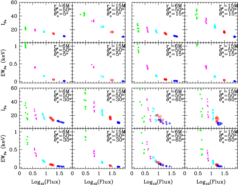
Figure 5: The intensity (I_Fe) and equivalent width (EW) of the iron K$\alpha$ line as a function of the direct flux for flares with different upward/downward (along $z$ direction defined in Appendix A) bulk velocities $\beta=-0.3$ (solid circles), $-0.1$ (solid squares), $0.1$ (open triangles), $0.3$ (open hexagons) and $0.5$ (open stars). Solid symbols represent downward (or inward in Figs. 6 and 8) bulk motion, while open symbols represent for upward (or outward in Figs. 6 and 8) bulk motion. The flare location and the observer inclination are labeled in each panel. Note that the eight points for each point style in each panel represent the flare azimuthal angles of $0\arcdeg$, $45\arcdeg$, $90\arcdeg$, $135\arcdeg$, $180\arcdeg$, $225\arcdeg$, $270\arcdeg$ and $315\arcdeg$, respectively. The intensity of the iron K$\alpha$ line and the direct flux are in arbitrary units. All the flares are assumed to have the same X-ray intrinsic luminosity and spectra.

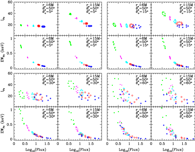
Figure 6: Legend as for Fig. 5 but for flares with inward/outward bulk motion (along $r$ direction).

We contrast the intensity and EW of the iron K$\alpha$ line with the direct flux from the flares with different location and bulk motions, but same intrinsic X-ray luminosity: Figures 5 and 7 show upward/downward bulk motion, and Figures 6 and 8 inward/outward bulk motion along the radius. In cases of flares with upward or outward bulk motions, the continuum flux increases with increasing bulk velocities of flares due to the beaming effect. It is interesting to note that a significant change in the direct flux does not necessarily mean a corresponding change in intrinsic X-ray luminosity. Instead, this change can be due to the change of the location and bulk velocity of flares. Moreover, a weak flare with a large bulk velocity towards the observer may appear as a bright flare, whereas a luminous flare closer to the central black hole with a small bulk velocity towards the observer may appear as a minimum period in the light curve. If a flare is very close to the black hole (with the radius $\lower 1.93747pt\hbox{$\;\buildrel<\over{\sim}\;$}10M$; for example, $6M$ in Figures 5 and 6), the number of photons impinging onto the disk decreases with increasing bulk velocity of the flare, but the trend is much weaker than the case of a flare located away from the black hole because of the dominance of the gravitational lensing effect over relativistic beaming. Therefore general relativistic effects cause only small difference in the total iron K$\alpha$ line flux for the most inner flares with different bulk velocities. However, the EW decreases rapidly with increasing bulk velocities of flares due to the rapid increase of the direct flux. If a flare is located above the approaching side of the disk, the total line flux is enhanced due to the Doppler effect. Conversely, the total line flux is repressed if the flare is located above the receding side of the disk. This asymmetric effect introduces a large scatter in the iron K$\alpha$ line flux and EW, especially for observers with large inclination angles and flares with large bulk velocities. For out-flowing flares, the direct flux is significantly affected by the angle between the flare bulk velocity vector and the line of sight. The direct flux is significantly enhanced for a flare moving towards the observer, i.e. located above the part of the disk facing the observer.

The most intriguing cases have flares with inward/outward bulk motions (e.g. Fig. 8) in which the total iron K$\alpha$ line fluxes are almost independent of the bulk velocity of flares (close to the black hole with the same intrinsic luminosity), and consequently the EW is inversely proportional to the continuum flux, for distant observers with inclination angles $\lower 1.93747pt\hbox{$\;\buildrel<\over{\sim}\;$}30\arcdeg$. It can be clearly seen in Figures 5 — 8 that a constant iron K$\alpha$ line flux can arise only for flares with low height above the disk and outward/inward (along the radius) bulk velocity. This requirement is possibly satisfied in realistic cases since it has been argued that the height of luminous magnetic flares cannot be much more than a few times the pressure height above a thin accretion disk (Nayakshin & Kazanas, 2001).

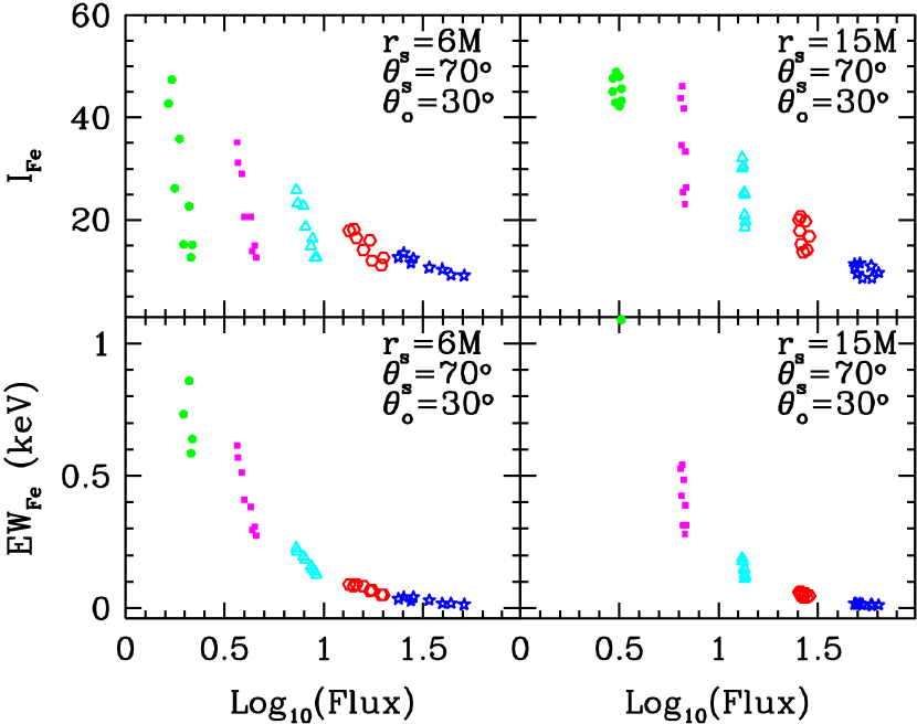
Figure 7: Legend as for Fig. 5 but for flares with $\theta_{\rm s}=70\arcdeg$ and only for a observer with inclination of $30\arcdeg$.

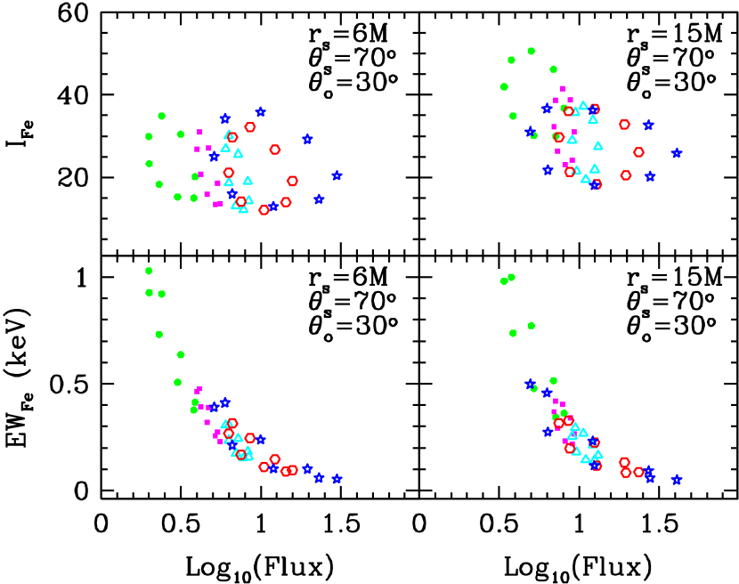
Figure 8: Legend as for Fig. 7 but for flares with inward/outward bulk motion (along $r$ direction). For each point style, generally the point with the largest I_Fe corresponds to the azimuthal angle of $\varphi_{\rm s}=270\arcdeg$  (on the approaching side of the disk), and with the symbols moving counterclockwise (or clockwise), the azimuthal angles change from 270°, 315°, 360°  (or 0°), 45°, 90°, 135°, 180°, to 225°  for downward/inward (or upward/outward) flares.

4 Applications and Discussion

4.1 Narrowness of the line profile

If only the effects of the bulk motion of flares on the profile and EW of the iron K$\alpha$ line are considered, a larger EW is found to be correlated with a more extended red wing of the iron K$\alpha$ line (see Figs. 1 and  2). This tendency is roughly consistent with observations: the larger the line EW, the more extended the red wing (e.g. Lubi$\acute{\rm n}$ski & Zdziarski, 2001, in the parameters obtained from the line modeling, a larger EW is accompanied by a smaller inner radius). Therefore, bulk motion in the corona can be introduced as a possible mechanism for producing the ‘narrowness’ of the iron K$\alpha$ line seen in some Seyfert 1 galaxies (see below); this is in addition to the generally introduced parameter of the truncation radius of the cold disk [the cold disk is truncated at a larger radius rather than the radius at the marginal stable orbit due to the transition of the inner disk to a hot geometrically thick and optically thin accretion flow or the high ionization of the disk material within this radius (Lubi$\acute{\rm n}$ski & Zdziarski, 2001, and references therein)]. It has been suggested that outflow/inflow in the corona provides a possible explanation for the $R-\Gamma$ relation (Beloborodov, 1999b). With the calculation in § 3.1.1, this out-flowing magnetic flares model is expected to consistently account for the ‘narrowness’ of the iron K$\alpha$ line profile, the variation of the EW, and the $R-\Gamma$ relation in some Seyfert 1 galaxies (Beloborodov, 1999b; Zdziarski, Lubi$\acute{\rm n}$ski & Smith, 2000; Lubi$\acute{\rm n}$ski & Zdziarski, 2001). Note that the “narrowness” of the line also depends on the location of the flare as seen in Fig. 1.

The model of a point source of X-ray emission along the rotation axis of the accretion disk is only an approximation to an accretion disk corona. Perhaps, a standard corona with upward/downward (or inward/outward) bulk motion is better approximated by a ring as shown in top (bottom) Fig. 4. Even with bulk velocity of 0.5 the line appears relatively broad with a red-wing extending down below 5 keV if the ring is located at a small radius, e.g. $6M$ (see Fig. 4 left panels). Here, one important question is: can an overall upward or outward bulk motion in the corona account for the ‘narrower’ iron K$\alpha$ line found in some Seyfert 1 galaxies? Done, Madejski & Życki (2000) found that IC4329A has a relatively narrow line which can be modeled using a disk line having an inner truncation radius of about $50M$ and EW of $210\pm 45$eV. NGC4593 was also found to have a relatively narrow iron K$\alpha$ line with an inner truncation radius of $30M$ (Lu & Wang, 2000). Even in NGC5548, the iron K$\alpha$ line emission region was found to be truncated at an inner radius of $15M$ (Chiang et al., 2000). The best-fit line profiles for NGC5548 and IC4329A are also shown (in Fig. 4) as light solid and light dotted lines, respectively. A significant fraction of the X-ray emission may come from the region within $15M$ in the thin disk$-$corona regime, which would indicate that the bulk motion in the corona is not the dominant factor making the line ‘narrower’ in some objects. As shown in Figure 4, obviously the observed ‘narrower’ line profile in IC4329A cannot be interpreted only by the corona bulk motion in this case. Other parameters (possibly the generally introduced inner truncation radius caused by the total ionization or disruption of the disk within this radius) are also still needed, or the corona in IC4329A is more extended and most of the X-ray emission comes from an outer region with radius of $\sim 50M$. For NGC5548, a narrow iron K$\alpha$ line which may be emitted from the broad line region or molecular torus, has been detected with the Chandra High-Energy Transmission Grating (Yaqoob et al., 2001). The corona bulk motion may account for the ‘narrower’ iron K$\alpha$ line in NGC5548 by removing the contribution from distant material. Here, even the X-ray emission may come mainly from the region around or within $15M$, and the ionization or disruption of the disk may not be necessary. Detailed models are beyond the scope of this paper.

4.2 The redshifted iron K$\alpha$ line from radio-loud quasars

With the observation of the Calibration and Payload Verification (Cal-PV) phase of XMM$-$Newton, a redshifted iron K$\alpha$ line at 6.15keV (quasar frame) has been found in the radio-loud quasar PKS0537-286 (redshift $z=3.104$) with an EW of 30eV, which suggests the existence of cold matter near the central black hole (Reeves et al., 2001). The overall spectral energy distribution of this object is dominated by a flat power-law X-ray emission with a spectral index of $\alpha\sim 0.27$, indicating that the dominant X-ray emission mechanism is the inverse Compton emission associated with a face-on relativistic jet (Reeves et al., 2001). The reflection fraction was constrained to be $R\simeq 0.25$ indicating the reflection material subtends a solid-angle much lower than the $2\pi$ expected from an accretion disk. Reeves et al. (2001) explained these features using two continuum emission components: a ‘Seyfert-like’ steep power-law component originating from the region near the accretion disk and associated with its reflection continuum, and a hard bright jet component with an X-ray flat slope. Generally, the radio jet is believed to be launched from the region close to the central black hole, which is possibly related to the ejecting X-ray plasma. These X-ray features in PKS0537-286 may also be explained in a unified model: the X-rays are emitted from the upward ejecting plasma near the central black hole (with radius of tens $M$) having an effective bulk velocity of $\sim 0.5-0.7$. The downward X-ray photons from the plasma are reflected by the accretion disk and thus produce the iron K$\alpha$ line with a small EW and the small reflection fraction due to the beaming effect. The redshifting of the line (from 6.4 keV to 6.15 keV) could also be explained as due to transverse-Doppler effect and gravitational redshift if this quasar is seen at a small inclination angle [radio-loud quasars are generally believed to be seen at a small inclination angle (Urry & Padovani, 1995), e.g. $\theta_{\rm o}\lesssim 15\arcdeg$, see also the upper panels of Fig. 1]. This X-ray emission region could be the base of the launching jet. Therefore, the iron K$\alpha$ line together with its reverberation could be a useful tool to probe the region of jet formation and to measure the initial velocity of the jet as well as the inclination of the disk in radio-loud quasars. This may reveal the physical connection between the jet properties and the cold accretion flow using future X-ray satellites (Constellation X-ray Mission and XEUS).

4.3 Explanation of the constant line flux in some objects

It is still a puzzle that the iron K$\alpha$ line flux appears to be constant in spite of strong continuum variation, and that the EW is anti-correlated with the continuum flux as in MCG-6-30-15 (Lee et al., 2000) and NGC5548 (Chiang et al., 2000). This was explained by the presence of a hot ionized skin of an accretion disk induced by thermal instability (Nayakshin, Kazanas & Kallman, 2000) or the resonant trapping followed by Auger destruction in an ionized disk which suppresses the emission of the iron K$\alpha$ line (Ballantyne, Ross & Fabian, 2001). However, ionization physics in the inner disk is unlikely to explain the behavior of iron K$\alpha$ line variation, at least in MCG-6-30-15 since the line profile suggests the existence of cold material within a radius of $5M$ (Iwasawa et al., 1999; Życki & R$\acute{\rm o}$ża$\acute{\rm n}$ska, 2001). The variation of the iron K$\alpha$ line profile in MCG-6-30-15 (and possibly also in NGC5548) may be explained by the out-flowing magnetic flares model in which the bulk motion and location of flares may vary [e.g. as discussed by Iwasawa et al. (1999)]. A subsequent question is: can the bulk motion and location of magnetic flares consistently explain the pattern of the variation in line intensity and EW corresponding to significant variations in continuum flux?

On occasion, the X-ray emission is dominated by a single (or a small number of) large flare(s) or neighboring flares (e.g. Poutanen & Fabian, 1999); but typically the X-ray emission may be a sum of a dozen or so overlapping flares. In the special case where the X-ray emission in an object at any given time is dominated by a single flare or neighboring flares in the inner region ($r\lower 1.93747pt\hbox{$\;\buildrel<\over{\sim}\;$}15M$), a significant non-axisymmetric illumination of the accretion disk is produced. If flares produced at different time have similar intrinsic X-ray luminosity, but move outward/inward with different bulk velocities, then the resulting iron K$\alpha$ line flux appears constant while the observed continuum flux undergoes rapid variability due to the beaming effect to a observer with a inclination $\lesssim 30\arcdeg$ (see Fig. 8). It is obvious that a constant iron K$\alpha$ line flux can also be obtained from a continuous corona (or a large number of overlapping flares) with varying bulk velocity in the region ($r\lower 1.93747pt\hbox{$\;\buildrel<\over{\sim}\;$}15M$, axisymmetric illumination) by averaging the symbols for the flares with same bulk velocity but different azimuthal angles in Fig. 8. Therefore, the model of out-flowing magnetic flares qualitatively explains the observational behavior of the iron K$\alpha$ line in MCG-6-30-15 (Lee et al., 2000) and NGC5548 (Chiang et al., 2000). These two objects are both constrained to have inclinations of $30\arcdeg$ from fits of the iron K$\alpha$ line profile with a relativistic disk line. The iron K$\alpha$ line in MCG-6-30-15 shows dramatic variability: it was narrow during a high-flux state and very broad during a deep-minimum flux, but the total line flux seems to be constant during the long ASCA observation in 1994 (Iwasawa et al., 1996); however, its blue part is shifted well below 6.4 keV during a short bright period in the long ASCA observation in 1997 (Iwasawa et al., 1999). Interestingly, the iron K$\alpha$ line profile has a huge red tail in the deep-minimum spectrum, and the line profile is without the 6.4 keV component during the bright period. These observations suggest that the X-ray source is very close to the central black hole and probably within radius of $6M$. If most of the X-ray is indeed emitted from the inner region with a typical radius of $6M$ in MCG-6-30-15, then a fluctuation of the bulk velocity of flares in the range $-0.1$ to $0.1$ (see Fig. 8), together with the non-axisymmetric illumination due to the difference in the location of flares (this non-axisymmetric illumination should be averaged in a long time interval) can account for the observational behavior of the iron K$\alpha$ line (Lee et al., 2000). Characterizing the iron K$\alpha$ line as a narrow plus a broad component, Iwasawa et al. (1996) found that the intensity of the narrow component correlates with the continuum flux, whereas the intensity of the broad component possibly anti-correlates with the continuum flux. This observational result is also qualitatively consistent with the out-flowing magnetic flare model. The X-ray emission in NGC5548 is also required — from the iron K$\alpha$ line profiles — to come from the inner egion around $15M$. However, the emission is more extended than that in MCG-6-30-15. The observed behavior of the iron K$\alpha$ line in NGC5548 (Chiang et al., 2000) may also be explained by the X-ray emission being dominated by moving magnetic flares with bulk velocity fluctuating around $0.2$ or $0.3$ at the region around or within $15M$.

It is interesting to note that if this model is correct it should apply in many different sources, including those observed at higher inclination angles. For example, in objects with high inclinations, i.e. Seyfert 2 galaxies, the iron K$\alpha$ line flux may not appear as a “constant” as in MCG-6-30-15 and NGC5548; instead, it may decrease with increasing continuum flux (see Fig. 6). The iron K$\alpha$ line flux may also not appear as a “constant” but anti-correlate with the continuum flux (see Fig. 5) in radio loud objects (e.g. quasars, which are generally believed to be observed at a small inclination angle) in which the out-flowing is upwards. The outflow/inflow mechanism can vary between sources observed at the same inclination angle (e.g. the radial outflow velocity may scale with the accretion rate unit in Eddington limit) as suggested above for MCG-6-30-15 and NGC5548. The case with a larger bulk velocities may have a smaller line EW, and also a narrower line profile due to a possible larger dissipation region.

4.3.1 Caveats and realities

Quantitatively, it is difficult to use the above model to explain the observational behavior of a constant iron K$\alpha$ line flux in MCG-6-30-15 and NGC5548 because the flare formation mechanism is not well known. (However, it is also a problem for other models, e.g. the totally ionized inner disk or the truncation of a thin disk in the inner region, since the formation of the X-ray corona or the dynamics of the truncation is not fully understood.) One major simplification in our calculation is that all flares are assumed to have the same intrinsic X-ray luminosity. However, the intrinsic X-ray luminosity of different flares may be different in realistic cases. Unfortunately, how flares are accelerated is not clear, as is the dependence of the bulk motion of flares on its intrinsic power. It is not yet known whether flares with larger bulk velocities tend to have larger intrinsic luminosity. The above model is viable only if the difference in the intrinsic power for flares with different bulk velocities is small (e.g., less than a factor of $1.5$). This may be satisfied for the avalanche-produced neighboring flares. Furthermore, the properties of flares may depend on their location. For example, the innermost flares may be more energetic or have a large bulk velocity than flares in the outer region. It is also possible that the innermost flares move with small outward bulk velocity due to the dominance of the gravitational field.

The spectral indices $\alpha$ of the X-ray continuum emitted from flares with different bulk motion and location should be different rather than the uniform value of $1.0$ adopted in our calculation. This difference will introduce some scatter in the EW and intensity of the iron K$\alpha$ line. This scatter will be less than 10 per cent for the observed variance of $0.2$ in the spectral index of MCG-6-30-15 ($\alpha\sim 0.8-1.0$, Lee et al., 2000) and NGC5548 ($\alpha\sim 0.75-0.95$, Chiang et al., 2000) (George & Fabian, 1991). It is not yet clear how the spectral index of the X-ray continuum from a flare depends on its bulk velocity and location. Without considering general relativistic effects, the photon index of the spectrum from magnetic flares with upward/downward bulk motion decreases with increasing bulk velocity (Beloborodov, 1999a, c; Malzac, Beloborodov & Poutanen, 2001). In an individual object, different low-height flares at different time may move with different outward/inward bulk velocities. The spectral variability is controlled by the parameters of temperature and optical depth of the Comptonizing medium, and the soft photons from the local disk radiation. It is possible that the temperature of the disk region where the flare is born is lower than that of the region surrounding it and less efficient at producing soft seed photons. So, in an individual object the flare with a higher outward bulk velocity may intercept more soft photons from the disk region surrounding the area where it is born since it moves away from the latter area more quickly, and will thus emit a harder continuum. Therefore, the fact that continuum spectra steepen with increasing continuum flux in MCG-6-30-15 (Lee et al., 2000) and NGC5548 (Chiang et al., 2000) may also be consistent with the out-flowing magnetic flare model used to explain the constant iron K$\alpha$ flux in these objects. Since it has been shown that systematic errors exist in the data fitting procedure of $R$ and $\Gamma$ (Vaughan & Edelson, 2000; Nandra et al., 2000), we do not try to explain the relation between $R$ and $\Gamma$ in MCG-6-30-15 and NGC5548. Other than the above complications, the difference in the bulk motion and location of magnetic flares could be the main cause of the observed constant iron K$\alpha$ line flux. Further relativistic calculations of the X-ray spectra from the flares with bulk motion near the central black hole are needed.

The behavior of a constant iron K$\alpha$ line flux in the presence of strong continuum variation can result from the combination of the effects of a strong gravitation field and relativistic beaming in the out-flowing magnetic flare model. This is only true for those objects in which the X-ray emission is concentrated in the innermost region with typical radii of $\lower 1.93747pt\hbox{$\;\buildrel<\over{\sim}\;$}15M$ and probably in objects where the iron K$\alpha$ line is also broad. The X-ray emission in some objects (e.g. IC4329A and NGC4593) must be emitted mainly in a region much larger than that in MCG-6-30-15 due to the observed ‘narrower’ iron K$\alpha$ line profile. Thus the expected variability of the iron K$\alpha$ line will not be similar to that in MCG-6-30-15 and NGC5548. If the behavior of constant iron K$\alpha$ line fluxes found in MCG-6-30-15 and NGC5548 is caused by ionization physics in the disk (Ross, Fabian & Young, 1999; Nayakshin, Kazanas & Kallman, 2000) rather than the relativistic effects described above, then similar variability would also be expected in those object with ‘narrower’ iron K$\alpha$ line. It is also possible that the model of out-flowing magnetic flares works for the objects like MCG-6-30-15 with neutral disk, but that the ionization model works for those objects with highly ionized accretion disks. We have to await future observations and detailed theoretical considerations to distinguish the out-flowing magnetic flare model from the model of highly ionized accretion disk.

5 Conclusions

We have performed fully relativistic calculations to reveal the effects of the bulk motion and location of magnetic X-ray flares above an untruncated accretion disk on the iron K$\alpha$ line properties, including the iron K$\alpha$ line profile, the EW, and the total line flux. The main conclusions are:

• The bulk motion of magnetic flares in the corona affects the iron K$\alpha$ line profiles. The red wing of iron K$\alpha$ line becomes less extended as the bulk velocity of the out-flowing magnetic flares increases. This effect is only significant for flares close to the central black hole.

• The EW of the iron K$\alpha$ line drops rapidly with increasing bulk velocity of the magnetic flares. In the out-flowing magnetic flare model, if the X-ray emission in an object is dominated by magnetic flares in the inner region ($r\lower 1.93747pt\hbox{$\;\buildrel<\over{\sim}\;$}15M$), it is difficult to get the ‘narrower’ lines observed in IC4329A, and a compatible EW. This suggests that the bulk motion cannot be the dominant factor causing the ‘narrowness’ in some AGNs.

• A fluctuation in the bulk velocity of the low-height out-flowing magnetic flares can account for the behavior of constant iron K$\alpha$ line fluxes and strong continuum variation observed in MCG-6-30-15 and NGC5548. This is especially interesting for the case of MCG-6-30-15, in which the iron K$\alpha$ line behavior is unlikely to be caused by the ionization of the accretion disk.

Appendix A Motion Constants:

The line element of the Kerr metric can be expressed in the form (Chandrasekhar, 1983)

$$ds^{2}=-{\rm e}^{2\nu}(dt)^{2}+{\rm e}^{2\psi}(d\varphi-\omega dt)^{2}+{\rm e}^{2\mu_{2}}dr^{2}+{\rm e}^{2\mu_{3}}d\theta^{2},$$ (A1)

where

$$\rm e^{2\nu} = A^{-1}\Delta\Sigma,$$

$$\rm e^{2\psi} = A\Sigma^{-1}\sin^{2}\theta,$$

$$\rm e^{2\mu_{2}} = \Delta^{-1}\Sigma,$$

$$\rm e^{2\mu_{3}} = \Sigma,$$ (A2)

$$A = (r^{2}+a^{2})^{2}-a^{2}\Delta\sin^{2}\theta,$$

$$\Delta = r^{2}+a^{2}-2r,$$

$$\Sigma = r^{2}+a^{2}\cos^{2}\theta,$$

$$\omega = \frac{2ar}{A},$$

and we have chosen the natural unit $G=c=M=1$ in Appendix A and B.

A four-velocity can be assigned at any point in this space-time:

$$u^{t} = \frac{dt}{ds}=\frac{\rm e^{-\nu}}{\sqrt{1-V^{2}}},$$

$$u^{\varphi} = \frac{d\varphi}{ds}=\varpi u^{t},$$

$$u^{r} = \frac{dr}{ds}=u^{t}v^{r},$$ (A3)

$$u^{\theta} = \frac{d\theta}{ds}=u^{t}v^{\theta},$$

where $\varpi=d\varphi/dt$, $v^{r}=dr/dt$ and $v^{\theta}=d\theta/dt$, and

$$V^{2}={\rm e}^{2\psi-2\nu}(\varpi-\omega)^{2}+{\rm e}^{2\mu_{2}-2\nu}(v^{r})^{2}+\rm e^{2\mu_{3}-2\nu}(v^{\theta})^{2}.$$ (A4)

In the locally non-rotating inertial frame, the four velocity is given by

$$u^{(t)} = \gamma=\frac{1}{\sqrt{1-V^{2}}},$$

$$u^{(\varphi)} = \gamma\beta_{\varphi}=\frac{{\rm e}^{\psi-\nu}(\varpi-\omega)}{\sqrt{1-V^{2}}},$$

$$u^{(r)} = \gamma\beta_{r}=\frac{{\rm e}^{\mu_{2}-\nu}v^{r}}{\sqrt{1-V^{2}}},$$ (A5)

$$u^{(\theta)} = \gamma\beta_{\theta}=\frac{{\rm e}^{\mu_{3}-\nu}v^{\theta}}{\sqrt{1-V^{2}}}.$$

Then the components of the comoving tetrad associated with this point are:

$${\bf e}_{(\hat{t})} = {\bf u},$$

$${\bf e}_{(\hat{\varphi})} = \gamma\beta_{\varphi}\rm e^{-\nu}\partial_{\it t}+[\gamma\omega\beta_{\varphi}\rm e^{-\nu}+(1+\beta_{\varphi}^{2}\frac{\gamma-1}{V^{2}})\rm e^{-\psi}]\partial_{\varphi}+$$

$$\beta_{\varphi}\beta_{r}\frac{\gamma-1}{V^{2}}\rm e^{-\mu_{2}}\partial_{\it r}+\beta_{\varphi}\beta_{\theta}\frac{\gamma-1}{V^{2}}\rm e^{-\mu_{3}}\partial_{\theta},$$

$${\bf e}_{(\hat{r})} = \gamma\beta_{r}\rm e^{-\nu}\partial_{\it t}+(\gamma\omega\beta_{r}\rm e^{-\nu}+\beta_{r}\beta_{\varphi}\frac{\gamma-1}{V^{2}}\rm e^{-\psi})\partial_{\varphi}+$$ (A6)

$$[1+\beta_{r}^{2}\frac{\gamma-1}{V^{2}}]\rm e^{-\mu_{2}}\partial_{\it r}+\beta_{r}\beta_{\theta}\frac{\gamma-1}{V^{2}}\rm e^{-\mu_{3}}\partial_{\theta},$$

$${\bf e}_{(\hat{\theta})} = \gamma\beta_{\theta}\rm e^{-\nu}\partial_{\it t}+(\gamma\omega\beta_{\theta}\rm e^{-\nu}+\beta_{\theta}\beta_{\varphi}\frac{\gamma-1}{V^{2}}\rm e^{-\psi})\partial_{\varphi}+$$

$$\beta_{\theta}\beta_{r}\frac{\gamma-1}{V^{2}}\rm e^{-\mu_{2}}\partial_{\it r}+[1+\beta_{\theta}^{2}\frac{\gamma-1}{V^{2}}]\rm e^{-\mu_{3}}\partial_{\theta}.$$

The trajectory of any photon emitted from a flare with bulk motion at this point can be specified by two motion constants, i.e. the component of angular momentum parallel to the symmetry axis $l$ and the Carter constant $Q$, which can be derived from the direction of the photon momentum and the comoving tetrad:

$$\cos\Psi = -\frac{{\bf p}_{\rm s}\cdot{\bf e}_{(\hat{r})}}{{\bf p}_{\rm s}\cdot{\bf u}_{\rm s}},$$

$$\sin\Psi\cos\Phi = -\frac{{\bf p}_{\rm s}\cdot{\bf e}_{(\hat{\theta})}}{{\bf p}_{\rm s}\cdot{\bf u}_{\rm s}},$$ (A7)

$$\sin\Psi\sin\Phi = -\frac{{\bf p}_{\rm s}\cdot{\bf e}_{(\hat{\varphi})}}{{\bf p}_{\rm s}\cdot{\bf u}_{\rm s}},$$

where ${\bf p}_{s}$ is the photon momentum at this location, and ${\bf u}_{s}$ is the bulk velocity of the flare at this point as expressed in ( A). Based on equations (A), (A) and (A), we can obtain

$$p_{\theta} = \frac{{\mathcal{K}}_{1}}{\mathcal{D}}l+\frac{{\mathcal{B}}_{1}}{\mathcal{D}},$$

$$p_{r} = \frac{{\mathcal{K}}_{2}}{\mathcal{D}}l+\frac{{\mathcal{B}}_{2}}{\mathcal{D}},$$ (A8)

where

$${\mathcal{K}}_{1} = \left[(1-\gamma)(f_{2}\beta_{\theta}^{2}+f_{1}f_{2}\beta_{r}\beta_{\theta}+f_{1}\beta_{\theta}\beta_{\varphi})+\gamma f_{2}V^{2}\right],$$

$$\times\frac{\Sigma}{A^{1/2}\sin\theta}+\gamma\omega V^{2}(f_{2}\beta_{\varphi}-f_{1}\beta_{\theta})\left(\frac{A}{\Delta}\right)^{1/2},$$

$${\mathcal{K}}_{2} = \left[(1-\gamma)(f_{1}f_{2}\beta_{r}^{2}+f_{1}\beta_{r}\beta_{\varphi}+f_{2}\beta_{r}\beta_{\theta})+\gamma f_{1}f_{2}V^{2}\right],$$

$$\times\frac{\Sigma}{(A\Delta)^{1/2}\sin\theta}+\gamma\omega f_{1}V^{2}(f_{2}\beta_{\varphi}-\beta_{r})\frac{A^{1/2}}{\Delta},$$

$${\mathcal{B}}_{1} = \gamma V^{2}\left(f_{1}\beta_{\theta}-f_{2}\beta_{\varphi}\right)\left(\frac{A}{\Delta}\right)^{1/2},$$

$${\mathcal{B}}_{2} = \gamma f_{1}V^{2}\left(\beta_{r}-f_{2}\beta_{\varphi}\right)\left(\frac{A^{1/2}}{\Delta}\right),$$ (A9)

$${\mathcal{D}} = \gamma f_{1}V^{2}+(1-\gamma)\left(f_{1}\beta_{\varphi}^{2}+f_{2}\beta_{\theta}\beta{\varphi}+f_{1}f_{2}\beta_{r}\beta_{\varphi}\right),$$

$$f_{1} = \frac{\cos\Psi}{\sin\Psi\cos\Phi},$$

$$f_{2} = \frac{\cos\Psi}{\sin\Psi\sin\Phi}.$$

Combining the equations (A-A) and the photon momentum equations

$$\frac{dt}{d\lambda} = \frac{A}{\Delta\Sigma}(1-\omega l),$$

$$\frac{dr}{d\lambda} = \pm\frac{1}{\Sigma}\left[(2r-al)^{2}+\Delta(r(r+2)-L)\right]^{1/2},$$

$$\frac{d\theta}{d\lambda} = \pm\frac{1}{\Sigma}\left(L-\frac{l^{2}}{\sin^{2}\theta}+a^{2}\cos^{2}\theta\right)^{1/2},$$ (A10)

$$\frac{d\varphi}{d\lambda} = \frac{A}{\Delta\Sigma}\left[\left(\frac{\Sigma-2r}{A}\right)\frac{l}{\sin^{2}\theta}+\omega\right]^{1/2},$$

we obtain the two motion constants $l$ and $Q$:

$$l = \frac{-Y+sgn(\pi-\Phi)\sqrt{Y^{2}-4XZ}}{2X},$$

$$Q = \frac{{\mathcal{B}}_{1}^{2}}{{\mathcal{D}}^{2}}+2\frac{{\mathcal{B}}_{1}{\mathcal{K}}_{1}}{{\mathcal{D}}^{2}}l+(\frac{{\mathcal{K}}_{1}^{2}}{{\mathcal{D}}^{2}}+\cot^{2}\theta)l^{2}-a^{2}\cos^{2}\theta,$$ (A11)

where

$$X = \frac{r^{2}-2r}{\Delta}+\Delta\frac{{\mathcal{K}}_{2}^{2}}{{\mathcal{D}}^{2}}+\frac{{\mathcal{K}}_{1}^{2}}{{\mathcal{D}}^{2}}+\cot^{2}\theta,$$

$$Y = \frac{4ar}{\Delta}+2\Delta\frac{{\mathcal{B}}_{2}{\mathcal{K}}_{2}}{{\mathcal{D}}^{2}}+2\frac{{\mathcal{B}}_{1}{\mathcal{K}}_{1}}{{\mathcal{D}}^{2}},$$ (A12)

$$Z = \Delta\frac{{\mathcal{B}}_{2}^{2}}{{\mathcal{D}}^{2}}+\frac{{\mathcal{B}}_{1}^{2}}{{\mathcal{D}}^{2}}-\frac{r^{4}+a^{2}r^{2}+2ra^{2}}{\Delta}-a^{2}\cos^{2}\theta.$$

The above expression (A) for the two motion constants can be applied to calculations of the photon trajectory of any point-like source with bulk motion in Kerr metric. If the source is static or has no bulk motion (i.e. $\beta_{\varphi}\rightarrow 0$, $\beta_{r}\rightarrow 0$ and $\beta_{\theta}\rightarrow 0$), this expression reduces to the simple one given by Karas, Vokrouhlick$\acute{\rm y}$ & Polnarev (1992).

For a flare above an accretion disk, where the flare bulk motion is observed in the locally non-rotating frame to be predominantly in the $z$-direction (say, upward or downward relative to the accretion disk), then the $z$-direction velocity is proportional to the $z$-direction unit vector:

$${\bf u}_{z}\propto{\bf n}_{z}={\rm e}^{-\mu_{2}}\cos\theta\partial_{\it r}-{\rm e}^{-\mu_{3}}\sin\theta\partial_{\theta}.$$ (A13)

The four velocity of the source is given by:

$${\bf u}=u^{t}({\partial_{\it t}}+\omega\partial_{\varphi}+V_{z}{\rm e}^{\nu-\mu_{2}}\cos\theta\partial_{\it r}-V_{z}{\rm e}^{\nu-\mu_{3}}\sin\theta\partial_{\theta}),$$ (A14)

where $V_{z}$ is the $z$-direction velocity relative to the locally non-rotating inertial frame. In the locally non-rotating inertial frame, the velocity components are:

$$\beta_{\varphi} = 0,$$

$$\beta_{r} = V_{z}\cos\theta,$$ (A15)

$$\beta_{\theta} = -V_{z}\sin\theta.$$

If the X-ray flare motion is dominated by motion in the $r$-direction (say, outward or inward), then the only non-zero velocity component in the locally non-rotating inertial frame is $\beta_{r}=V_{r}$. It is also possible that the flare co-rotates with the disk while other direction motion can be neglected (i.e. $\beta_{r}=\beta_{\theta}=0$). The motion constants in (A) are then equivalent to the ones given by Ruszkowski (2000).

Note that any choice of the value of $V_{z}$ or $V_{r}$ must meet the requirement of $V^{2}<1$ in order that the source follows a time-like world-line.

For the special case that the flare is on axis and has only $r$-/$z$-direction motion (i.e. $\theta\rightarrow 0$ and $\beta_{\varphi}=\beta_{\theta}=0$), the two motion constants reduce to:

$$l = 0,$$

$$Q = \frac{r^{4}+a^{2}r^{2}+2a^{2}r}{\Delta}-\frac{A}{\Delta}\left(\frac{\beta_{r}+\cos\Psi}{\beta_{r}\cos\Psi+1}\right)^{2}.$$ (A16)

Appendix B Illumination of the disk and the direct observed continuum flux

We assume the X-ray luminosity in the source comoving frame to be isotropic and in the form of a power law $L_{E_{e}}=L_{0}E^{-\alpha}_{\rm e}$, where $E_{\rm e}$ is the photon energy in the source comoving frame. The Monte-Carlo simulation shows that the anisotropic effect is very weak for multiple scattering which dominates the hard X-ray emission, although the soft X-ray emission is significantly anisotropic in the case of single scattering approximation (Janiuk, Czerny & Życki 2000). In the frame rotating with the disk, including the ‘k-correction’, the illuminating flux on the disk element ($r\rightarrow r+dr$, $\varphi\rightarrow\varphi+d\varphi$) with an incident angle of $\theta_{\rm in}$ ($\cos\theta_{\rm in}=-{\bf p}\cdot{\bf n}/{\bf p}\cdot{\bf u_{\rm d}}$, where ${\bf n}$ is the equator normal) is given by (e.g. Yu & Lu 2000; Ruszkowski 2000):

$$F^{\rm ill}_{\rm d}(E_{\rm d},\theta_{\rm in};r,\varphi)=L_{0}g^{1+\alpha}_{\rm sd}E^{-\alpha}_{\rm d}\gamma^{-1}\frac{f_{\rm sd}}{d\varphi dr}(\frac{\Delta}{A})^{1/2},$$ (B1)

where $f_{\rm sd}$ is the fraction of total photons which corresponds to the grid elements defined by $d\varphi dr$, $g_{\rm sd}$ is the redshift factor for a photon propagating from the source to the disk grid elements given by

$$g_{\rm sd}=\frac{{\bf p}_{\rm s}\cdot{\bf u}_{\rm s}}{{\bf p}_{\rm d}\cdot{\bf u}_{\rm d}},$$ (B2)

and $\gamma$ is the Lorentz factor of the relative motion of the disk element and the locally non-rotating inertial frame. For $r\geq r_{\rm ms}$, where $r_{\rm ms}$ is the radius of the last stable orbit, the $\gamma$ factor is given by:

$$\gamma=(1-V^{(\varphi)2})^{-1/2},\ \ \ V^{(\varphi)}=\frac{A}{(\Sigma\Delta)^{1/2}}(\Omega_{d}-\omega),$$ (B3)

where $\Omega_{\rm d}=1/(a+r^{3/2})$ is the rotation velocity of the disk (see Cunningham 1975). The incident photon number intensity is then $N_{E_{\rm d}}^{\rm in}(E_{\rm d},\theta_{\rm in};r,\varphi)=F^{\rm ill}_{\rm d}(E_{\rm d},\theta_{\rm in};r,\varphi)/E_{\rm d}$.

Note in equation (B1) the power index of $g$ is $(1+\alpha)$, which is different from $(2+\alpha)$ in Yu & Lu (2000) where the total flux is considered.

If a distant observer is located at $(r_{\rm o},\theta_{\rm o},\varphi_{\rm o})$ with collecting area on the $r=r_{\rm o}$ sphere equal to

$$\delta S=r^{2}_{\rm o}\sin\theta_{\rm o}\delta\varphi_{\rm o}\delta\theta_{\rm o},$$ (B4)

the direct flux component from the flare received by the observer is analogously given by

$$F_{\rm dir}(E_{\rm obs})=L_{0}g^{1+\alpha}_{\rm so}E^{-\alpha}_{\rm o}\frac{f_{\rm so}}{\delta S},$$ (B5)

where $f_{\rm so}$ is the fraction of the total number of emitted photons intersecting the observers collecting area, and $g_{\rm so}$ is the redshift factor of a photon propagating from the flare to the observer and is given by a formula similar to equation (B2):

$$g_{\rm so}=\frac{{\bf p}_{\rm s}\cdot{\bf u}_{\rm s}}{{\bf p}_{\rm o}\cdot{\bf u}_{\rm o}}.$$ (B6)

References

- Agol & Krolik (2000) Agol, E., & Krolik, J. H. 2000, ApJ, 528, 161
- Armitage, Reynolds & Chiang (2001) Armitage, P. J., Reynolds, C. S., & Chiang, J. 2001, ApJ, 546, 868
- Ballantyne, Ross & Fabian (2001) Ballantyne, D. R., Ross, R. R., & Fabian, A. C. 2001, MNRAS, in press (astro-ph/0102040)
- Basko (1978) Basko, M. M. 1978, ApJ, 223, 268
- Beloborodov (1999a) Beloborodov, A. M. 1999a, MNRAS, 305, 181
- Beloborodov (1999b) Beloborodov, A. M. 1999b, ApJ, 510, L123
- Beloborodov (1999c) Beloborodov, A. M. 1999c, in ASP Conf. Ser., High Energy Processes in Accreting Black Holes, ed. J. Poutanen & R. Svensson (San Francisco: ASP), P295
- Branduardi-Raymont et al. (2001) Branduardi-Raymont, G., Sako, M., Kahn, S. M., Brinkman, A. C., Kaastra, J. S., & Page, M. J. 2001, A&A, 365, L140
- Campana & Stella (1993) Campana, S., & Stella, L. 1993, MNRAS, 264, 395
- Chandrasekhar (1983) Chandrasekhar, S. 1983, The Mathematical Theory of Black Holes. Oxford University Press, Oxford, p. 68
- Chiang et al. (2000) Chiang, J., Reynolds, C. S., Blaes, O. M., Nowak, M. A., Murray, N., Madejski, G., Marshall, H. L., & Magdziarz, P. 2000, ApJ, 528, 292
- Cunningham (1975) Cunningham, C. T. 1975, ApJ, 202, 788
- Dabrowski et al. (1997) Dabrowski, Y., Fabian, A. C., Iwasawa, K., Lasenby, A. N., & Reynolds, C. S. 1997, MNRAS, 288, L11
- Dabrowski & Lasenby (2001) Dabrowski, Y., & Lasenby, A. N. 2001, MNRAS, 321, 605
- Done, Madejski & Życki (2000) Done, C., Madejski, G. M., & Życki, P. 2000, ApJ, 536, 213
- Esin, McClintock & Narayan (1997) Esin, A. A., McClintock, J. E., & Narayan, R. 1997, ApJ, 489, 865
- Fabian et al. (1989) Fabian, A. C., Rees, M. J., Stella, L., & White, N. E. 1989, MNRAS, 238, 729
- Fabian et al. (1995) Fabian, A. C., Nandra, K., Reynolds, C. S., Brandt, W.N., Otani, C., Tanaka, Y., Inoue, H., & Iwasawa, K. 1995, MNRAS, 277, L11
- Fabian et al. (2000) Fabian, A. C., Iwasawa, K., Reynolds, C. S., & Young, A. 2000, PASP, 112, 1145
- Field & Rogers (1993) Field, G. B., & Rogers, R. D. 1993, ApJ, 403, 94
- Galeev, Rosner & Vaiana (1979) Galeev, A. A., Rosner, R., & Vaiana, G. S. 1979, ApJ, 229, 318
- George & Fabian (1991) George, I. M., & Fabian, A. C. 1991, MNRAS, 249, 352
- Ghisellini, Haardt & Matt (1994) Ghisellini, G., Haardt, F., & Matt, G. 1994, MNRAS, 267, 743
- Haardt (1993) Haardt, F. 1993, ApJ, 413, 680
- Hartnoll & Blackman (2000) Hartnoll, S. A., & Blackman, E. G. 2000, MNRAS, 317, 880
- Iwasawa et al. (1996) Iwasawa, K., et al. 1996, MNRAS, 282, 1038
- Iwasawa et al. (1999) Iwasawa, K., Fabian, A. C., Young, A. J., Inoue, H., & Matsumoto, C. 1999, MNRAS, 306, L19
- Janiuk Czerny & Życki (2000) Janiuk, A., Czerny, B., & Życki, P.T. 2000, MNRAS, 318, 180
- Karas, Vokrouhlick & Polnarev (1992) Karas, V., Vokrouhlick, D., & Polnarev, A. G. 1992, MNRAS, 259, 569
- Kojima (1991) Kojima, Y. 1991, MNRAS, 250, 629
- Laor (1991) Laor, A. 1991, ApJ, 376, 90
- Lee et al. (2000) Lee, J. C., Fabian, A.C., Reynolds, C. S., Brandt, W. N., & Iwasawa, K. 2000, MNRAS, 318, 857
- Lu & Wang (2000) Lu, Y., & Wang, T. 2000, ApJ, 537, L103
- Lubiski & Zdziarski (2001) Lubiski P., & Zdziarski, A. A. 2001, MNRAS, 323, L37
- Malzac, Beloborodov & Poutanen (2001) Malzac, J., Beloborodov, A. M., & Poutanen, J. 2001, MNRAS, 326, 417
- Martocchia & Matt (1996) Martocchia, A., & Matt, G. 1996, MNRAS, 282, L53
- Martocchia, Karas & Matt (2000) Martocchia, A., Karas, V., & Matt, G. 2000, MNRAS, 312, 817
- Matt & Perola (1992) Matt, G., & Perola, G. C. 1992, MNRAS, 259, 433
- Matt, Perola & Piro (1991) Matt, G., Perola, G. C., & Piro, L. 1991, A&A, 247,25
- Matt et al. (1992) Matt, G., Perola, G. C., Piro, L., & Stella, L. 1992, A&A, 257,63 (Erratum: 1992, A&A, 263, 453)
- Matt, Fabian & Ross (1993) Matt, G., Fabian, A. C., & Ross, R. R. 1993b, MNRAS, 262, 179
- Matt, Fabian & Ross (1996) Matt, G., Fabian, A. C., & Ross, R. R. 1996, MNRAS, 278, 1111
- Matt (2000) Matt, G. 2000, astro-ph/0007105
- Merloni & Fabian (2001) Merloni, A., & Fabian, A. C. 2001, MNRAS, 321, 549
- Nandra & Pounds (1994) Nandra, K., & Pounds, K. A. 1994, MNRAS, 268, 405
- Nandra et al. (1997) Nandra, K., George, I. M., Mushotzky, R. F., Turner, T. J., & Yaqoob, T. 1997, ApJ, 477, 602
- Nandra et al. (2000) Nandra, K., Le, T., George, I. M., Edelson, R. A., Mushotzky, R. F., Peterson, B. M., & Turner, T. J. 2000, ApJ, 544, 734
- Nayakshin & Kazanas (2001) Nayakshin, S., & Kazanas, D. 2001, ApJ, 533, L141
- Nayakshin, Kazanas & Kallman (2000) Nayakshin, S., Kazanas, D., & Kallman, T. 2000, ApJ, 537, 833
- Pariev & Bromley (1998) Pariev, V. I., & Bromley, B. C. 1998, ApJ, 508, 590
- Pounds et al. (1990) Pounds, K. A., Nandra, K., Steward, G. C., Geroge, I.M., & Fabian, A. C. 1990, Nature, 344, 132
- Poutanen & Fabian (1999) Poutanen, J., & Fabian, A. C. 1999, MNRAS, 306, L31
- Poutanen, Krolik & Ryde (1997) Poutanen, J., Krolik, J. H., & Ryde, F. 1997, MNRAS, 292, L21
- Rauch & Blandford (1994) Rauch, K. P., & Blandford, R. D. 1994, ApJ, 421, 46
- Reeves et al. (2001) Reeves, J. N., Turner, M. J. L., Bennie, P. J., Pounds, K. A., Short, A., O’Brien, P. T., Boller, Th., Kuster, M., & Tiengo, A., 2001, A&A, 365, L116
- Reynolds (2000a) Reynolds, C. S. 2000a, ApJ, 533, 811
- Reynolds (2000b) Reynolds, C. S. 2000b, astro-ph/0009503
- Reynolds & Begelman (1997) Reynolds, C. S.,& Begelman, M. C. 1997, ApJ, 488, 109
- Reynolds & Fabian (1997) Reynolds, C. S., & Fabian, A. C. 1997, MNRAS, 290, L1
- Reynolds et al. (1999) Reynolds, C. S., Young, A. J., Begelman, M. C., & Fabian, A. C. 1999, ApJ, 514, 164
- Romanova et al. (1998) Romanova, M. M., Ustyugova, G. V., Koldoba, A. V., Chechetkin, V. M., & Lovelace, R. V. E. 1998, ApJ, 500, 703
- Ross & Fabian (1993) Ross, R. R., & Fabian, A. C. 1993, MNRAS, 261, 74
- Ross, Fabian & Brandt (1996) Ross, R. R., Fabian, A. C., & Brandt, W. N. 1996, MNRAS, 278, 1082
- Ross, Fabian & Young (1999) Ross, R. R., Fabian, A. C., & Young, A. J. 1999, MNRAS, 306, 461
- Ruszkowski (2000) Ruszkowski, M. 2000, MNRAS, 315, 1
- Stella (1990) Stella, L. 1990, Nature, 375, 659
- Tanaka et al. (1995) Tanaka, Y., et al. 1995, Nature, 344, 747
- Urry & Padovani (1995) Urry, C. M., & Padovani, P. 1995, PASP, 107, 803
- Vaughan & Edelson (2000) Vaughan, S., & Edelson, R. 2001, ApJ, 548, 694
- Yaqoob et al. (2001) Yaqoob, T., George, I. M., Nandra, K., Turner, T. J., Serlemitsos, P. J., & Mushotzky, R. F. 2001, ApJ, 546, 759
- Young & Reynolds (2000) Young, A. J., & Reynolds, C. S. 2000, ApJ, 529, 101
- Young, Ross & Fabian (1998) Young, A. J., Ross, R. R., & Fabian, A. C. 1998, MNRAS, 300, L11
- Yu & Lu (2000) Yu, Q., & Lu, Y. 2000, MNRAS, 311, 161
- Zdziarski, Lubiski & Smith (2000) Zdziarski, A. A., Lubiski, P., & Smith, D. A. 1999, MNRAS, 303, L11
- Życki & Czerny (1994) Życki, P. T., & Czerny, B. 1994, MNRAS, 266, 653
- Życki & Rżaska (2001) Życki, P. T., & Rżaska, A. 2001, MNRAS, 325, 197