Investigation of clustering of galaxies, clusters and superclusters by the method of correlation Gamma-function

Abstract

Using the apparatus of correlation Gamma-function (“conditional density”), we have analyzed spatial clustering of objects from several different samples of galaxies, clusters and superclusters. On small scales the distribution of objects obeys a power law drop of density with a power index of 0.9–1.5. On a scale of $\sim 30$ Mpc for independent samples of bright galaxies and clusters of galaxies we have detected a pronounced break in the slope of the Gamma-function with a power index decreasing to $\sim 0.3$. The clustering is much less pronounced in the region from 40 to 100 Mpc, and there is reason to suppose that the distribution of objects changes to homogeneous on scales larger than 100 Mpc. This is indicated by the slope of the Gamma-function close to 0 for a sample of rich clusters of galaxies up to 250 Mpc.

The slope of the Gamma-function prior to the break, which characterizes the degree of clustering of matter, changes essentially and in a complex manner when passing to brighter (massive) objects. This suggests that the large-scale structure of the visible Universe even on small scales is considerably more complex than the fractal distribution described by one dimension (monofractal).

Key words:   cosmology: observations — galaxies: formation — galaxies: statistics

1 Introduction

One of the principles on which standard cosmological models are based is homogeneity of distribution of matter on large scales (Peebles, 1983). A direct indication of such a character of distribution of matter in the observed Universe is, for instance, the homogeneity and anisotropy of CMB radiation. At the same time, the investigators of the large-scale structure have discovered inhomogeneities in the distribution of visible matter on scales to 100 Mpc (IAU Symp., 1978; Geller & Huchra, 1989). Within the frames of the present-day knowledge there are two main large-scale structure models: a homogeneous model with fluctuations of density of finite amplitudes and a fractal model characterized by self-similarity of structures of the observed Universe in a certain interval of scales. A question on scales of extension of fractal structures is being debated. According to Davis (1997), the self-similarity properties of distribution of galaxies manifest themselves but to 10 Mpc. Pietronero et al. (1997) advocated the idea that a maximum scale of clustering cannot be reached by the present-day surveys of galaxies and clusters of galaxies, the fractal properties in the distribution of matter are observed to $\sim 150$ Mpc and there are signs of extension of the fractal structure to $\sim 1000$ Mpc.

There are several key stages in the history of origin and development of knowledge of fractal (self-similar) type of distribution of matter. Having noticed the sequence of clustering (galaxies, groups, clusters, superclusters), de Vaucouleurs (1970) provided an observational substantiation of the model of hierarchical clustering which could explain the power, with a slope $\gamma\sim 1.7$, decreasing of density with increasing radius (de Vaucouleurs diagram). By 1982 Mandelbrot (1977, 1982) had extended these ideas and introduced a mathematically rigorous notion of fractals and proposed, following from general considerations, a fractal dimension $D=1$ for the Universe.

About 20-year work over the redshift surveys, increasingly deeper and complete, made it possible to see in the distribution of galaxies the structures and voids of different shape (Huchra et al., 1983), the filling of the volume by objects with measured $z$ still more clearly defined the features noticed previously (Fairall, 1998). The maps of the distribution of galaxies in space of redshifts (CfA1 survey (Huchra et al., 1983), the first deep two-dimensional (slice) CfA2 survey (Geller & Huchra, 1989) and others) were consistent with intuitive ideas of stochastic fractal point distributions in three-dimensional space: extended “coherent regions” of increased density, voids occupying a considerable part of the volume, general “clumpy” and irregular pattern of distribution.

The more detailed construction of the three-dimensional pattern of the nearest regions of the Universe gave impetus to development of a variety of statistical methods (Borgani, 1995; El-Ad et al., 1996; Paladin & Vulpiani, 1987; Plionis & Valdarnini, 1992) of isolation and study of different structures in the distribution of objects in the Universe (such as voids, filaments, superclusters, “walls”). As distinct from the two-point correlation function, these methods reveal more finely characteristic morphological properties of the structures. The methods of search for fractal (scale-invariant) properties of matter distribution were executed mathematically (Borgani, 1995; Pietronero, 1987; Coleman & Pietronero, 1992).

2 Mathematical apparatus

If the mean density in the volume under study is not determined, i.e. it varies considerably with increasing working volume up to scales characterizing the volume under study, the standard statistical method of analysis of the large-scale structure, the two-point correlation function ($\xi$-function) (Peebles, 1983; Davis & Peebles, 1983; Boerner & Mo, 1990; Klypin & Kopylov, 1983; Dalton et al., 1992) will then yield a result dependent on the parameters of the sample and the way of calculation. For instance, it has been noted that the “correlation scale” $r_{0}$ grows with increasing volume of the sample (Einasto et al., 1986; Coleman & Pietronero, 1992).

Pietronero et al. (1988) and Coleman & Pietronero (1992) noticed that if the given sample does not include the scales where the amplitude of clustering is small, i.e. the distribution is homogeneous (the scatter of the number of galaxies in distant equal volumes is described by the Poissonian statistics), then the parameters of the $\xi$-function do not show the real amplitude and the limiting scale of clustering, and proposed another method of calculation of the correlation function of density, the so-called Gamma-function (hereafter Gamma) or the “conditional density” (Coleman & Pietronero, 1992) used in statistical physics for analysis of non-analytical structures with large-scale density correlations. Pietronero and his co-workers (Pietronero et al., 1997; Sylos Labini et al., 1996, 1997; Montuori et al., 1997; Sylos Labini et al., 1998) had been using this method for over 10 years to study the distribution of astrophysical objects and concluded that fractal structures are extended to scales 100–150 $h^{-1}$ Mpc, and from indirect data (relation between “radial” density and distance from ESP survey) even to $\rm\sim 1000\,h^{-1}$ Mpc (Pietronero et al., 1997).

The papers of Pietronero and his colleagues found a broad response. Cosmological models were proposed which took account of the fractality (Baryshev, 1981; Baryshev et al., 1994) as an essential part of the Universe picture (interpretation of redshift as a gravitation effect which is determined by the global inhomogeneity of the Universe but not by the expansion of space). Controversy developed as to the scales of extension of the fractal structure (Davis, 1997; Pietronero et al., 1997). Nevertheless, among the researchers of the large-scale structure only Pietronero’s group keeps holding “radical” viewpoints of the enormous extension (up to 1000 Mpc) of the fractal law of density variation with distance, which is described by the single dimension $D$ (Mandelbrot, 1977; Feder, 1988).

The fractal methods are difficult to apply to the study of distribution of galaxies and clusters of galaxies because the existing samples represent the distribution of a finite number of points in a finite volume, whereas the fractal properties in terms of mathematics are determined at the limit of infinity. For the “physical” or “dynamical” fractal a large (but finite) interval of scales between the lower and upper limits of manifestation of self-similarity properties is necessary ( McCauley, 1997).

The condition “volume limited” should be met in order that all regions of the sample be represented with equal rights, that is, from every object one could “see” any other. For samples of galaxies this condition is realized when the objects, whose absolute stellar magnitude is larger than that of the faintest galaxies at the far limit of the sample, are rejected.

It is important to note that the ideology of construction of the Gamma calls for abandoning a priori assumptions concerning the properties of the distribution of the sample objects. Thus for the method to be used, careful preliminary work is required on the creation of a sample of homogeneously selected objects with sharply defined spatial boundaries. The scales to which the Gamma can be calculated are restricted by the radius of a maximum sphere with the centre in the object of the sample, which can still fall within the boundaries of the sample.

The Gamma is variation of the mean density of objects as the volume under study increases. The differential and integral Gamma-functions are determined as follows:

$$\Gamma(r)=\frac{1}{N}\sum\limits_{i=1}^{N}\frac{1}{4\pi r^{2}\Delta}\int\limits_{r}^{r+\Delta}n(r_{i}-r)dr,$$ (1)

$$\Gamma^{*}(r)=\frac{1}{N}\sum\limits_{i=1}^{N}\frac{1}{4\pi r^{3}}\int\limits_{0}^{r+\Delta}n(r_{i}-r)dr,$$ (2)

where $n(r)=\frac{1}{N}\sum\limits_{i=1}^{N}\delta(r_{i}-r)$ is the numerical density.

The integral function ($\Gamma^{*}$) averages the contribution of different scales and therefore, with the presence of properties of a monofractal in the distribution, it smoothes fluctuations and allows the dimension of the distribution to be measured with a higher accuracy than the differential function. At the same time the integral function is not very sensitive to change of the type of distribution. The differential function, in principle, registers better change of the mode of distribution than the integral function does, and in this sense it is more informative, but at the same time it is more susceptible to fluctuations.

In some cases the form of the Gamma has a simple interpretation. For the monofractal with the single dimension $D$ (“filling of the volume” occurs, on the average, in the same manner on all scales for all objects) the relationship between the number of objects in a sphere and its radius, $N(r)=Br^{D}$, is satisfied. In the general case $D\leq 3$. For a homogeneous distribution the number of points in the volume is directly proportional to the volume ($D=3$).

The average density in a sphere of radius $R_{s}$ placed in a given fractal structure or, for instance, in a  uniform   distribution   is $\langle n\rangle=\frac{N(R_{s})}{V(R_{s})}=\frac{3B}{4\pi}R_{s}^{-(3-D)}$. At $D<3$ the average density $\langle n\rangle$ is a diminishing function of radius $R_{s}$ and $\langle n\rangle\rightarrow 0$ at $R_{s}\rightarrow\infty$ is satisfied for each point regarded as the centre of the sphere of radius $R_{s}$. For the homogeneous distribution ($D=3$) the average density is constant and independent of the volume it is measured in.

In the case of a “pure” monofractal structure, $\Gamma^{*}$ must change according to a power law with the slope of the straight line in the plot $\log(\Gamma^{*})-\log(r)$, which is defined by the fractal dimension of the set. If the fractal properties manifest themselves only to a certain scale $\lambda_{0}$ with transition to uniformity on larger scales, the relations:

$$\Gamma(r)=\frac{DB}{4\pi}r^{-(3-D)},r<\lambda_{0},$$

$$\Gamma(r)=\frac{DB}{4\pi}\lambda_{0}^{-(3-D)},r\geq\lambda_{0}$$

are satisfied. The Gamma function is represented here by definition in the form $\Gamma(r)=\frac{1}{4\pi r^{2}}\frac{dN}{dr}$ and $N(r)=Br^{D}$.

When analysing the real distribution, it should be borne in mind that even if the points of the integral Gamma fall well on a straight line in the region of drop of the “conditional density”, it does not suggest that the properties of the monofractal are present in the distribution. Analysis of artificial distributions shows that the power law Gamma diminishing with the index $-\gamma$ is a necessary, but not a sufficient condition for fractality of the distribution with the dimension $D=3-\gamma$. Nevertheless, the power law character of the Gamma in the interval of scales, where it is defined with sufficient reliability, admits a fractal interpretation. Other attributes of fractality, for instance, self-similarity of the structures, the proportion of voids in the volume, require a special study by suitable methods.

The paper consideres the relations between $\log(\Gamma)$ and $\log(r)$, $\log(\Gamma^{*})$ and $\log(r)$. The angular coefficient of the approximation line, which is plotted on the chosen region of the $\log(r)$ variation, defines the correlation dimension of the distribution (co-dimension). The greater slope (corresponding to the smaller dimension implies, on the average, a stronger decrease of density inside the volume and therefore a higher clustering of objects. The horizontal regions of the plot point, in the general case, to uniformity of distribution of objects in the sample on corresponding scales.

Fig. 1 shows the expected behaviour of the Gamma in transition from fractal clustering on scales less than $\lambda_{0}$ to uniform distribution on larger scales. The figure illustrates the informativeness of using the Gamma in searching for the scale of change of the condition of clustering $\lambda_{0}$, provided that $R_{s}$ is well larger than $\lambda_{0}$.

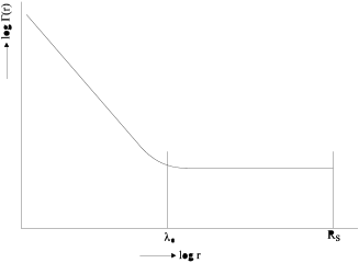
Figure 1: $\lambda_{0}$ is the maximum scale of extension of correlations. $R_{s}$ is the limiting scale of calculation of gamma-functions.

3 The way of calculation

• The boundaries of the region of the highest completeness are denoted (the zone of incompleteness along the radial axis and the region of strong interstellar extinction are usually excluded).

• The density of the objects that fall within the spherical layer $r_{0}<r<r_{0}+\Delta$ around each object, that is, the density at a given distance from the object of the sample for the differential Gamma, and the density in spheres of radius $r_{0}$ with the centres in the objects of the sample for the integral Gamma are calculated (the centres of the spheres are not included in the counts, i.e. the density of the “neighbours” is measured). The calculations are averaged. The results are presented on a logarithmic scale in the form of the relations $\log(\Gamma)$ and $\log(r_{0})$, $\log(\Gamma^{*})$ and $\log(r_{0})$.

• If a part of some sphere falls outside the sample limits with increasing working radius $r_{0}$, the sphere is then excluded from the calculations. Thus, with increasing working radius, only the spheres with the centres progressively nearing to that of the volume containing the sample are involved in the calculations. The calculations are terminated when the number of remaining spheres is $N_{sp}<10$.

The method of calculation implemented in the present paper differs from the variant used by Pietronero and his colleagues but in insignificant details (the step of increasing the working radius, the number of finite spheres at which the calculations are terminated and others).

We call this method of Gamma calculation “classical” as distinct from modifications using various kinds of weighting of the regions of spheres falling outside the sample limits (Lemson & Sanders, 1991; Andreani et al., 1991) and other procedures allowing more effective utilization of the whole volume of the sample. The demerit of the method is that the sample objects are unequal in rights since the objects located at the boundaries fall out rapidly from the calculation as the centres of spheres. Therefore the result on large scales is strongly dependent on the distribution of a small number of objects near the centre of the volume being studied. From our estimates the Gamma remains informative at a minimum number, 100–200, (depending on the volume) of objects, left in the sample. A detailed examination of the question is presented in Sylos Labini et al. (1996).

The problem of determining the error of approximation of the Gamma slope in the region, where the power law decrease of density is observed, is difficult to overcome because there is no “etalon” of distribution for the Gamma, as distinct from the statistics which compare in some way the distribution of a sample with uniform one. The dispersion of the Gamma calculations with respect to the mean does not, strictly speaking, indicate the error of the mean value of the Gamma since for an arbitrary distribution, for instance, fractal, the spread in values may be natural, and only the mean Gamma values are of significance. The “bootstrap” method (Ling et al., 1986; Mo et al., 1992) may possibly give correct estimates of the errors.

The distances for all samples of galaxies were taken Euclidean and were determined by the Hubble law $R=V_{0}/H_{0}$, where $V_{0}$ is the radial velocity, and $H_{0}$ is the Hubble constant. The K-correction was not taken into account.

When changing the redshift values to metric distances for the clusters (Abell and APM), the following formula was used:

$$R=\frac{c}{H_{0}}\frac{q_{0}+(q_{0}-1)(\sqrt{1+2q_{0}z}-1)}{q_{0}^{2}(1+z)}.$$ (3)

The values $H_{0}=100$ km/s/Mpc for the Hubble constant and $q_{0}=0.1$ for the deceleration parameter were used in the calculation by this formula.

4 Description of samples and results of calculations

To analyse the Gamma behaviour, diverse data were chosen which represented samples of physically isolated structures of luminous matter (galaxies, clusters, superclusters), allowing the clustering on scales from 50 kpc to $\sim 200$ Mpc to be estimated.

4.1 Local Volume

This is a sample of nearby galaxies with radial velocities less than 500 km/s with respect to the Local Group centroid. The original list made by Kraan-Korteweg and Tammann (1979) numbered 179 objects. Further it was substantially complemented by Karachentsev (the most complete compilation can be found in Makarov’s thesis (2000). We will emphasize that this is the only sample with photometric estimates of distances of galaxies. We used a sample of 330 objects. Of these 330 objects, 193 galaxies have photometric estimates of distances, for 47 objects the distances are taken from their membership in known groups, and only for the rest of the objects Hubble distances ($H_{0}=70$ km/s/Mpc) were used.

A supergalactic “disk”, in which 80 % of galaxies are concentrated, is dominated in the distribution of the Local Volume galaxies. This is a flat structure that occupies the centre of the volume and becomes more dense in the direction toward Virgo. Practically all known groups of galaxies of the Local Volume (the Local Group, M81, NGC 5128+NGC 5236 (Centaurus), NGC 4244+NGC 4736 (Canes Venatici), M101) are located in the disk. In the northern direction (in supergalactic coordinates) the “Local Void” detected by Tully is situated. It takes approximately half of the volume in question. From Karachentsev’s estimates there are no galaxies brighter than $M_{B}=-13^{m}$ in absolute magnitude in this region.

The results of the Gamma-analysis are presented in Figs. 2 and 3. The slope $\gamma\sim 1.2$ in the Local Volume is likely to be defined by the distribution geometry. The expected slope for a pancake-type structure is $\gamma\sim 1$. The test with the use of random “mixing” of galaxies in the “disk” does not change essentially the result of the Gamma-analysis. That is, strictly speaking, the distribution of galaxies in the Local Volume is largely inhomogeneous because of the presence of the “Local Void”, but not fractality. It is likely that the slope of the Gamma towards small scales remains practically up to the size of a large galaxy ($\sim 50$ kpc) owing to the dwarf companions of the most massive galaxies.

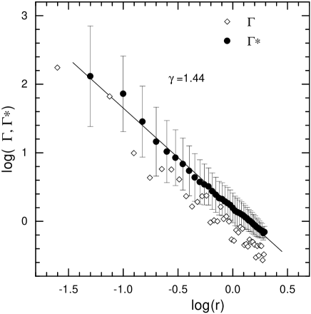
Figure 2: The “Disk” of the Local Volume $R_{\mbox{s}}=2.0$ Mpc.

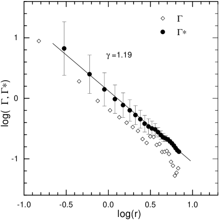
Figure 3: The Local Volume $R_{\mbox{s}}=7.15$ Mpc.

4.2 CfA2 and SSRS2 catalogues of galaxies

CfA2 (a subsample from the UZC catalogue (Falco et al., 1999)). The catalogue of Zwicky with $m_{\rm Zw}=15.5^{m}$ formed the basis for the redshift survey of the Center for Astrophysics. Systematical measurements of redshifts were started in 1978. By the present time, 14632 spectra have been obtained within the frame of the CfA2 project. As to redshifts, the survey (96 % completeness with $m_{\rm Zw}=15.5^{m}$) comprises 13150 galaxies with measured radial velocities. About 30 % of data were taken by the authors from the literature. In the regions $20^{h}<\alpha<4^{h}$ (south), $8^{h}<\alpha<17^{h}$  (north), $-2.5^{\circ}<\delta<50^{\circ}$ (12925 galaxies) the catalogue completeness reaches 98 %.

SSRS2 (July, 1998, da Costa et al., 1998). 5369 galaxies to the apparent magnitude $15.5^{m}$, which cover 1.7 sterad of the southern hemisphere, are picked up from the list of nonstellar objects catalogued in HST GSC. The accuracy of determination of the positions is $\sim 1\hbox{${}^{\prime\prime}$}$. The error of photometric magnitudes is $0.3^{m}$. The system of magnitudes is homogeneous over the sky and corresponds to magnitudes measured at an isophote level of $\sim 26^{m}\hbox{\hbox to0.0pt{$\sqcap$\hss}$\sqcup$}^{\prime\prime}$. The radial velocities are accurate to $\sim 40$ km/s. The survey completeness in redshifts is 99 % to the $15.5^{m}$ apparent magnitude.

Since SSRS2 is in fact the extension of the CfA2 survey to the southern sky, we united in the analysis the adjacent southern and northern regions of CfA2 and SSRS2 to obtain the following samples:

north:  CfA2 ($0^{\circ}<\delta<90^{\circ}$, $7^{h}<\alpha<18^{h}$, $b^{II}>15^{\circ}$) + SSRS2 ( $\delta<0^{\circ}$, $b^{II}>35^{\circ}$),

south:  CfA2($-2.5^{\circ}<\delta<50^{\circ}$, $20^{h}<\alpha<4^{h}$, $b^{II}<-15^{\circ}$) + SSRS2( $-60^{\circ}<\delta<-2.5^{\circ}$, $b^{II}<-40^{\circ}$).

The results of the Gamma-analysis of four subsamples for the northern and southern sky are presented in Figs. 4, 5, 6 and 7. From the independent northern and southern samples one can see a pronounced break at 20–30 Mpc. The large extent of the region after the break suggests that the break is due to the distribution properties, but not the boundary effects. It should be noted that the results of the Gamma in the northern and southern parts are practically coincident, though the morphological distinctions (the presence of isolated structures) are different for all samples.

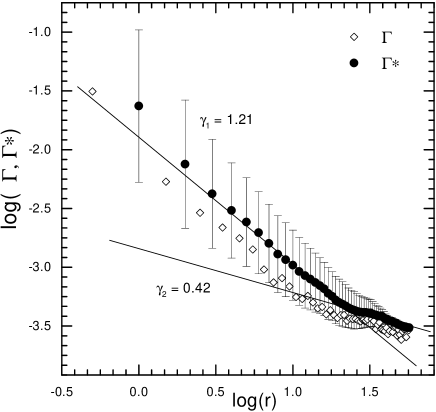
Figure 4: CfA2+SSRS2 north $R_{\mbox{lim}}=140$ Mpc.

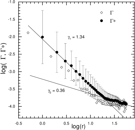
Figure 5: CfA2+SSRS2 north $R_{\mbox{lim}}=160$ Mpc.

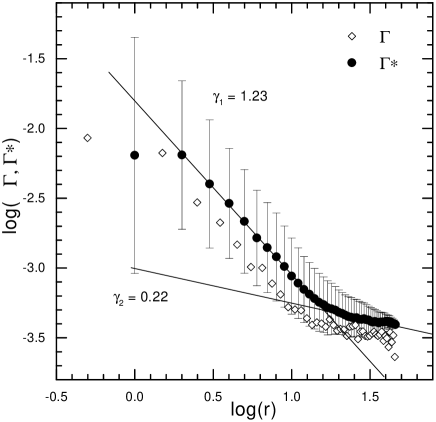
Figure 6: CfA2+SSRS2 south $R_{\mbox{lim}}=140$ Mpc.

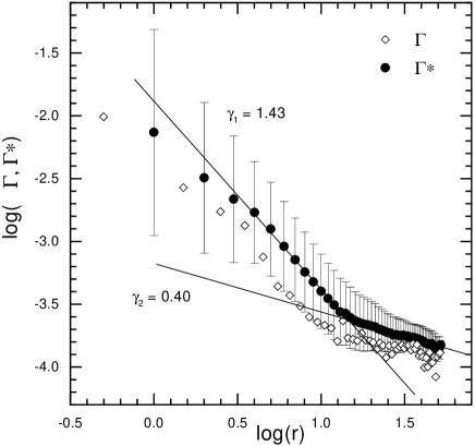
Figure 7: CfA2+SSRS2 south $R_{\mbox{lim}}=160$ Mpc.

4.3 APM clusters

The catalogue of APM clusters (Dalton et al., 1992, 1997) is the first sufficiently large catalogue of clusters of galaxies formed with the aid of an automated procedure of isolation of objects based on the APM catalogue of galaxies to b${}_{\rm j}=20.5^{m}$ in the southern sky region: $-72.5\hbox{${}^{\circ}$}<\delta<-17.5\hbox{${}^{\circ}$}$, $20.5^{h}<\alpha<5.6^{h}$. The richness of clusters and the characteristic brightness of galaxies were determined together in a circle of radius $0.75~{}h^{-1}$ Mpc, which is twice as small as the one used by Abell. In the opinion of the authors of the catalogue this has improved considerably its homogeneity. A total of 957 clusters with estimates of $z<0.12$ are found in this region (Dalton et al., 1997). For 374 of them the redshifts are determined spectroscopically, including 55 clusters with measured $z>0.12$. The completeness of measurements of $z$ for richer clusters is considerably higher than for poor. For this reason, we have chosen for the analysis the APM clusters with the richness $\mathcal{R}\geq 54$, which corresponds approximately to the richness $R\geq 0$ (or $N_{A}\geq 30$) for Abell clusters. In total such clusters number 346. Among them 43 have measured $z>0.12$, and we have not considered them, for 217 $z<0.12$, and for 86 there are available only estimated $z$ (by definition smaller than 0.12). The completeness of measurements of redshifts for the subsample from the APM catalogue is about 72%.

According to the way of compilation, the clusters have been catalogued with the highest statistical completeness in a certain middle interval of $z$. A small number of nearby clusters might not be included in the catalogue because of large angular dimensions, and a considerable number, increasing towards the far boundary of the volume, of distant clusters because of the decreasing with distance contrast of the cluster and errors in the determination of the characteristic stellar magnitude of galaxies of the cluster.

As can be seen from Figs. 8 and 9, the Gamma shows a particularly pronounced break at R$\simeq$32 Mpc. The slope $\gamma_{2}\approx 0.3$, i.e. we see a correlation of the distribution on scales $>$30 Mpc, but the clustering is insignificant here. The interval from the point of break top to the limit of calculation of the Gamma is considerable, from 30 Mpc to $\sim 100$ Mpc. The incompleteness of the measured $z$ does not affect the location of the break; it is only the slope of $\Gamma^{*}$ that changes prior to the break point.

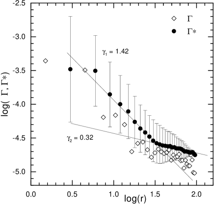
Figure 8: APM clusters with measured z, $N=217$.

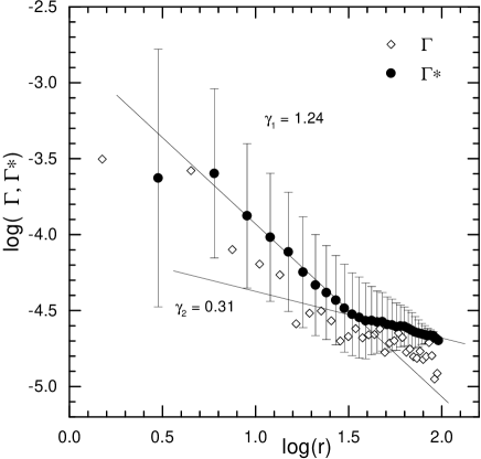
Figure 9: APM clusters with measured (217) and estimated (86) z, $N=303$.

4.4 Rich Abell clusters in the “Northern Cone”

In this sample are included all Abell’s clusters of galaxies (Abell et al., 1989) with richness $N_{A}\geq 70$ ($N_{A}=50-79$ corresponds to the richness class $R=1$) which are located in the region $b^{II}>40^{\circ}$, for which $z\leq 0.24$ either measured or estimated according to Leir and van den Bergh (1977). For 247 (77%) out of 321 clusters there are available spectroscopically measured $z$, about 33% measurements of $z$ were made with the 6 m telescope in the course of the programme on studying distribution of rich clusters in the “Northern Cone” (Kopylov et al., 1988; Kopylov, 1999). For such rich clusters (remind that the clusters with $N_{A}\geq 80$ belong to the classes of richness $R\geq 2$) at high galactic latitudes ($b^{II}>40^{\circ}$) the catalogue of Abell, perhaps, may not be considered as strongly distorted by the effects of incompleteness which could influence seriously the shape of the Gamma. At the present time, this sample of clusters is likely to be the best one for our purpose both in its completeness and homogeneity and in coverage of the volume of space.

The subsample of rich clusters that we have obtained allows one to follow the behaviour of the Gamma in a very wide and probably in the most interesting range of scales, 10–250 Mpc, in which from theoretical reasoning and from the available data an asymptotic transition to the homogeneous distribution of objects in space must be observed. It is exactly this behaviour of the Gamma that has been detected (see Figs.10 and 11). After the region of power law drop in density with the slope $\gamma\approx 1.5$, starting from $\approx 40$ Mpc, a transitional interval follows with gradual decrease in slope, and beginning with the radius $\geq 120$ Mpc, the distribution of clusters does not practically differ from homogeneous up to a limiting radius of 250 Mpc.

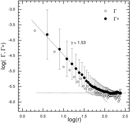
Figure 10: Rich Abell clusters with measured z, $N=247$.

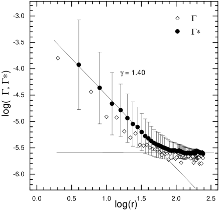
Figure 11: Rich Abell clusters with measured (247) and estimated (74) z, $N=321$.

The use of the sample in which only measured $z$ are present (incomplete sample) does not change essentially the Gamma shape and shows that the result from the complete (in the sense of location of objects in the volume) sample is not practically distorted by the fact that for part of the clusters estimated $z$ have been taken. The inclusion into the sample of clusters with estimated $z$ leads only to reduction of the steepness of the slope on small scales, that is, “blurring” of clustering of clusters on the scales of superclusters occurs.

4.5 Superclusters of galaxies

The catalogue of superclusters of Einasto et al. (1997) which covers the region $R<350$ Mpc, $|b^{II}|>17^{\circ}$ was constructed by the method of percolation using Abell clusters of richness $R\geq 0$ both with measured and estimated redshifts $z<0.12$. The percolation radius is 24 Mpc. A total of 220 superclusters were revealed. Einasto et al. (1997) pointed out that superclusters are located at the nodes of a quasi-regular lattice.

As distinct from clusters of galaxies, superclusters represent nonvirialized systems numbering from 2 to 36 (for the richest of all — the Shapley supercluster) Abell clusters. The great difference in population and, therefore, in sizes is due to the procedure of construction of the catalogue. This may, in principle, introduce unpredictable variations in the correlation properties of the sample since the superclusters considered in the calculations as point objects may actually be strongly anisotropic systems, for revealing of which the method of percolation is just the most suitable. Nevertheless, the Gamma calculation for the superclusters of Einasto et al. is of interest as an independent method of control of clustering of matter on sufficiently large scales ($\leq 150$ Mpc).

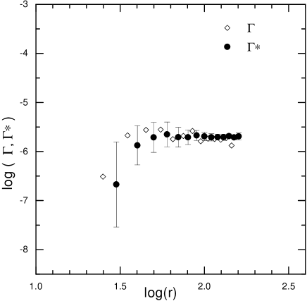
Figure 12: Einasto superclusters, north.

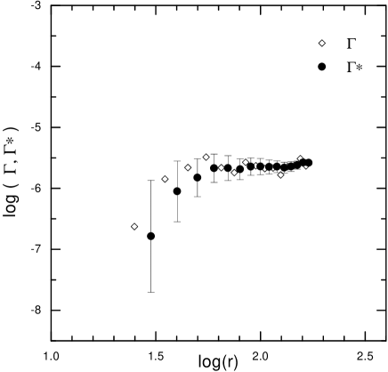
Figure 13: Einasto supercluster, south.

Table 1: Parameters of various samples

$R_{\mbox{lim}}$	$M_{\mbox{lim}}$	N	$R_{\mbox{s}}$	$\gamma_{1}$	$R_{\mbox{break}}$	$\gamma_{2}$
(Mpc)			(Mpc)		(Mpc)
Local volume ($H_{0}=70$)
7.15	-13.0	198	7.15	1.19	–	–
Local “disk” ($H_{0}=70$)
2.0	-13.0	146	2.0	1.44	–	–
CfA2+SSRS2, north ($H_{0}=100$)
180	-20.78	212	69	1.41	24	0.52
160	-20.52	458	69	1.34	20	0.36
140	-20.23	959	61	1.21	23	0.42
120	-19.90	1691	52	0.98	19	0.46
100	-19.50	2610	43	0.86	16	0.40
CfA2+SSRS2, south ($H_{0}=100$)
180	-20.78	194	64	1.53	25	0.11
160	-20.52	339	58	1.43	15	0.40
140	-20.23	611	52	1.23	17	0.22
120	-19.90	1056	44	0.97	20	0.19
100	-19.50	1517	39	1.01	19	0.19
APM-clusters, richness $\mbox{$\mathcal{R}$}\geq 54$ ($H_{0}=100$)
1)with measured and evaluated $z$
339		303	105	1.24	32	0.31
2) only with measured $z$
339		217	105	1.42	32	0.32
Abell clusters, richness $N_{A}\geq 70$ ($H_{0}=100$)
1) with measured and evaluated $z$
638		321	246	1.40	$\approx 40$	$\sim 0.3$
					$\geq 120$	$\simeq 0$
2) only with measured $z$
638		247	246	1.53	$\approx 40$	$\sim 0.3$
					$\geq 120$	$\simeq 0$
Einasto superclusters, north ($b^{II}>15^{\circ}$) ($H_{0}=100$)
350		98	164	–	(40)	0
Einasto superclusters, south ($b^{II}<15^{\circ}$) ($H_{0}=100$)
350		122	173	–	(40)	0

In Figs. 12 and 13 is displayed the Gamma calculated for the northern and southern subsamples of superclusters. On scales larger than the percolation radius, immediately after the appearance of the “signal”, that is when a sufficient number of objects fall within the sphere and spherical layers, the Gamma shows directly homogeneity of distribution of superclusters in both the southern and northern regions beginning with a scale of about 40 Mpc, that is, approximately from the scale on which the Gamma of clusters of galaxies shows the first break. The second, a less pronounced break (or a feature on the curve of the Gamma variation) on a scale of about 120 Mpc may likely be associated with transition to quasi-regular distribution of the superclusters on a lattice with a period of about 125 Mpc (Einasto et al., 1997). Note that evidence to this scale of clustering in the spatial distribution of rich clusters was also obtained in measuring the correlation function of rich compact clusters in the “Northern Cone” (Kopylov et al., 1988).

5 Discussion of results

In Table 1 are collected the principal results of the analysis. The first four columns present the basic parameters of the samples of objects. $R_{\mbox{lim}}$ is the far boundary of the sample along the radial coordinate. $M_{\mbox{lim}}$ is the limitation on absolute magnitude for the “volume limited” sample, which corresponds to $R_{\mbox{lim}}$. $N$ is the number of objects in the sample. $R_{s}$ is the radius of the maximum sphere falling inside the boundaries of the sample. In the last three columns are given the parameters of the simplest model that we have used to describe the Gamma behaviour: “power law drop” of density (index $\gamma_{1}$) — break ($R_{\mbox{break}}$) — change of the mode of clustering ($\gamma_{2}$)”.

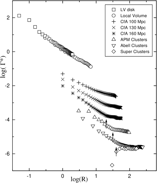
Figure 14: A master figure of Gamma functions for different samples. Squares and circles show the behaviour of the Gamma for samples of the Local Volume and Supergalactic Disk, respectively. The crosses of different form are for the northern part of the samples CfA2+SSRS2, for the depths 100, 130, 160 Mpc. The triangles are for APM clusters. The inverted triangles are for Abell clusters. The diamonds designate the Gamma for Einasto superclusters.

The results of investigation of all principal samples are displayed in Fig. 14 in order to make more convenient their comparison with one another and to attempt to reveal common laws of clustering throughout the investigated range of scales.

In Fig. 14 one can see an approximately “coordinated” break over different samples including the spheres with $R>30-40$ Mpc (the first arrow). From the galaxies of the northern part of the sample CfA2+SSRS2 the extension of the region of the Gamma after the break suggests that the break is most likely caused not by the boundary effects, but rather by the properties of distribution. For APM clusters the Gamma has a break at $\approx 30$ Mpc, the limiting scale is 105 Mpc. The tendency of behaviour of this type Gamma (break and transition to other mode of clustering) is terminated by deep samples of rich clusters and superclusters, nearly complete “leveling out” of the Gamma (the second and third arrows) is observed. A trend of slope $\gamma_{1}$ (prior the break) is noticeable over all samples, the dynamics and causes of which still remain to be solved. Formally, the power law of the drop of density begins with scales $\sim 50$ kpc, immediately after the size of a huge galaxy.

We used rather heterogeneous data, even though the results obtained from different samples basically agree with each other in the main features, which allows some general conclusions to be drawn concerning the character of behaviour of the Gamma on different scales.

1. The shape of the correlation Gamma function points to the density variation according to a power law.

2. The power index on small scales (prior the break) changes within 0.9–1.5. In principle, this corresponds to fractal distribution, but the scatter in slopes for different samples of objects of different nature makes questionable the possibility of describing a large-scale structure by a single fractal dimension.

3. Manifestations of fractality have been revealed on scales spanning nearly 3 orders of magnitude — from 50 kpc to 30 Mpc.

4. Systematic variations of the Gamma parameters obtained from CfA2+SSRS2 galaxies require additional investigation, although the tendency to “leveling out” of the Gamma at $R>20-25$ Mpc for brighter objects is consistent with the results for clusters (brighter galaxies concentrate towards the centres of clusters).

5. On scales 30–40 Mpc, in the cases where the Gamma is calculated to scales well larger than 40 Mpc, a break is seen in the behaviour of the Gamma (index $\gamma\leq 0.5$) which implies the change of the condition and, possibly, a physical mechanism of clustering.

6. From 30 to 100–120 Mpc the clustering is likely to occur, since on these scales isolated structures (Great Wall, voids, etc.) are observed, but it is insignificant, for when increasing the scales, the density drops slightly. Probably, the contrast (amplitude) of inhomogeneities on these scales is already small.

7. An asymptotic transition to homogeneity $\gamma_{2}\rightarrow 0$ might be supposed, mainly from the distribution of rich clusters and superclusters on scales 40–120 Mpc.

As a whole, the correlation Gamma-function is quite an interesting and informative way of describing a large-scale structure. It should be noted, however, that the influence of selection effects on the shape of the Gamma is still not clearly studied. A study is required of model samples with expected properties of the Gamma and properties introduced by real selection effects (for instance, the density gradient along the radial coordinate).

The limitation of scales of calculation by spheres located inside the sample boundaries does not solve the problems of boundary conditions completely, because the Gamma becomes dependent on the location of significant structures inside the sample boundaries. This points to the necessity of careful selection of objects and choice of sample boundaries. The incompleteness of the sample may diminish the statistical significance of the result of Gamma application. Other methods should be involved to confirm the interpretation.

Nevertheless, it can be argued with assurance that our results of application of the Gamma function are in fair agreement with theoretical considerations of the finitness of the range of scales with the fractal type of correlation of density and of gradual decrease of contrast of inhomogeneities with increasing volume of the region of the Universe being studied.

• The authors express their gratitude to Yu.V. Baryshev, V.A. Hagen-Thorn and I.D. Karachentsev for keen interest they took in the work and assistance in its accomplishment. A.Tikhonov is grateful for support through the grant “Integration” N A0007.

References

- [1] Abell G.O., Corwin H.C. & Olowin R.P., 1989, Astrophys. J. Suppl. Ser., 70, 1
- [2] Andreani P., Cristiani S. & La Franca, F., 1991, Mon. Not. R. Astron. Soc., 253, 527
- [3] Baryshev Yu.V., 1981, Astrofis. Issled. (Izv. SAO), 14, 24
- [4] Baryshev Yu.V., Sylos Labini F., Montuori M., Pietronero L., 1994, Vistas in Astronomy, 38, 419
- [5] Boerner, G. & Mo, H.J., 1990, Astron. Astrophys., 227, 324
- [6] Borgani S., 1995, Physics Reports, 251, 1
- [7] Coleman P.H. & Pietronero L., 1992, Physics Reports, 213, 311
- [8] Dalton G.B., Efstathion G., Maddox S.J., Sutherland W.J., 1992, Astrophys. J., 390, L1
- [9] Dalton G.B., Maddox S.J., Sutherland W.J., Efstathion G., 1997, Mon. Not. R. Astron. Soc., 289, 263
- [10] Davis M. & Peebles P.J.E., 1983, Astrophys. J., 267, 465
- [11] Davis M., 1997, Critical Dialogues in Cosmology. Proceedings of a Conference held at Princeton, New Jersey, 24-27 June 1996, Singapore: World Scientific, edited by Neil Turok, 13
- [12] da Costa L.N., Willmer C.N.A., Pellegrini P.S., et al., 1998, Astron. J., 116, 1
- [13] de Vaucouleurs G., 1970, Science, 167, 1203
- [14] Einasto J., Klypin A.A. & Saar E., 1986, Astrophys. J., 302, L1
- [15] Einasto M., Tago E., Jaaniste J., et al., 1997a, Astron. Astrophys. Suppl. Ser., 123, 119
- [16] Einasto J., Einasto M., Gottloeber S., et al., 1997b, Nature, 385, 139
- [17] El-Ad H., Piran T. & da Costa L.N., 1996, Astrophys. J., 462, L13
- [18] Fairall A.P., 1998, Large-scale Structure of the Universe, New York: Wiley
- [19] Falco E.E., Kurtz M.J., Geller M.J., et al., 1999, Publ. Astr. Soc. Pacific, 111, 438
- [20] Feder E., 1988, Fractals, Moscow, Mir
- [21] Geller M.J. & Huchra J.P., 1989, Science, 246, 897
- [22] Huchra J., Davis M., Latham D., Tonry J., 1983, Astrophys. J. Suppl. Ser., 52, 89
- [23] IAU Symp., N 79, 1978, Large-scale structure of the Universe, eds.: Longair M.S. & Einasto J., D. Reidel publishing company
- [24] Karachentsev I.D. 1994, Astron. Astrophys. Transact., 6, 1
- [25] Klypin A.A., Kopylov A.I., 1983, Pis’ma Astron. Zh., 9, No.2, 75
- [26] Kopylov A.I., Kuznetsov D.Yu., Fetisova T.S. & Shvartsman V.F., 1988, in: J.Audouse et al.(eds), Large-Scale Structure of the Universe, 129
- [27] Kopylov A.I., 1999, Private communication
- [28] Kraan-Korteweg R.C. & Tammann G.A., 1979, Astron. Nachr., 300, 181
- [29] Lemson G. & Sanders R., 1991, Mon. Not. R. Astron. Soc., 252, 319
- [30] Leir A.A. & van den Bergh S., 1977, Astrophys. J. Suppl. Ser., 34, 381
- [31] Ling E.N., Barrow J.D. & Frenk C.S., 1986, Mon. Not. R. Astron. Soc., 223, 21P
- [32] Makarov D.I., 2000, Galaxy motion on small and large scales (in Russian) Ph.D. Thesis, SAO RAS
- [33] Mandelbrot B., 1977, Fractals: Form, Chance and Dimensions, San Francisco: Freeman
- [34] Mandelbrot B., 1982, The Fractal Geometry of Nature, New York: Freeman
- [35] McCauley J.L., 1997, Are galaxy distribution scale-invariant? (a perspective from dynamical systems theory), astro-ph/9703046
- [36] Mo H.J., Jing Y.P., Boerner G., 1992, Astrophys. J., 392, 452
- [37] Montuori M., Sylos Labini F. & Amici A., 1997, Correlation properties of cluster distribution, astro-ph/9705123
- [38] Paladin G. & Vulpiani A., 1987, Physics Reports, 156, 147
- [39] Peebles P.J.E., 1983, The Universe structure on large scales, Moscow, Mir
- [40] Pietronero L., Montuori M. & Sylos Labini F., 1997, Critical Dialogues in Cosmology. Proceedings of a Conference held at Princeton, New Jersey, 24-27 June 1996, Singapore: World Scientific, edited by Neil Turok, 24
- [41] Pietronero L., 1987, Physica A, 144, 257
- [42] Pietronero L., et al., 1988, Phys. Rev. Lett., 61, 861
- [43] Plionis M. & Valdarnini R., 1992, Astrophys. J., 398, 12
- [44] Sylos Labini F., Gabrielli A., Montuori M., Pietronero L., 1996, Physica A, 226, 195
- [45] Sylos Labini F., Pietronero L. & Montuori M., 1997, Frequently asked questions about fractals, Proceedings of the Workshop “Astro-particle Physics”, Ringberg Castle, 15–19 October 1996, astro-ph/9701156
- [46] Sylos Labini F., Montuori M. & Pietronero L., 1998, Physics Reports, 293, 61