A Supernova Brane Scan

Abstract

We consider a ‘brane-world scenario’ recently introduced by Dvali, Gabadadze and Porrati, and subsequently proposed as an alternative to a cosmological constant in explaining the current acceleration of the universe. We show that, contrary to these claims, this particular proposal is already strongly disfavoured by the available Type Ia Supernovae, Cosmic Microwave Background and cluster data.

1 Introduction

At a time when observational cosmologists are finally pinning down some crucial cosmological parameters (Perlmutter et al., 1997, 1999; Riess et al., 1998; de Bernardis et al., 2000; Lange et al., 2001; Netterfield et al., 2001; Hanany et al., 2000; Balbi et al., 2000; Stompor et al., 2001; Halverson et al., 2001; Pryke et al., 2001; Percival et al., 2001), theoretical cosmologists have increased and diversified their efforts to try to provide some more solid connections between particle physics and cosmology.

In this context, a topic of much recent interest has been that of the so-called ‘brane-world scenarios’ (Arkani-Hamed, Dimopoulos & Dvali, 1998; Randall & Sundrum, 1999; Binétruy et al., 2000; Maartens, 2001; Rubakov, 2001). The general principle behind such models is that the ordinary particles live on a three-dimensional surface (commonly called a 3-brane, or simply ‘the brane’), which is embedded in a larger space (‘the bulk’, which may or may not be compact and might even have an infinite volume) on which gravity can propagate. An observer on the brane will measure four-dimensional gravity up to some corrections which, given the weakness of gravity, can in general be made small enough not to conflict with observations without tweaking with model parameters too much.

At present the topic is young enough that the main drive is still to try to explore all remotely viable model-building possibilities without worrying too much about the consequences. However, some of the proposed models are already developed enough that they can start to be put through the sieve of specific cosmological observations. In this paper we will provide what we believe to be the first detailed analysis of this kind for a brane world scenario.

We will consider a particular solution of a brane world scenario originally introduced by Dvali, Gabadadze & Porrati (2000), and further studied in (Deffayet, 2001; Deffayet, Dvali & Gabadadze, 2001)—we shall refer to it as the DGP model for simplicity. It’s a five-dimensional brane-world model with a non-compact, infinite-volume extra dimension. The usual four-dimensional gravity is recovered on the brane for scales below a ‘characteristic radius’ $r_{c}$, due to a four-dimensional Ricci scalar being induced on the brane. However, at larger scales this becomes sub-dominant, and one will effectively see five-dimensional Einstein-Hilbert gravity.

The above effect can obviously have dramatic cosmological implications. A particularly interesting solution was first found by Deffayet (2001)—and then generalized by Dick (2001)—and then further studied in (Deffayet, Dvali & Gabadadze, 2001). It describes a universe which at late times is accelerated on scales larger than $r_{c}$. This is an effect of the bulk gravity, in the sense that observers on the brane will see no cosmological constant. Hence this is another interesting alternative way to explain the current acceleration of the universe, which is strongly indicated by Type Ia supernova observations (Perlmutter et al., 1997, 1999; Riess et al., 1998), without resorting to a cosmological constant—for earlier alternative explanations, see (Dev, Sethi & Lohiya, 2000; Behnke et al., 2001; Mannheim, 2001). Note that, unlike most other known brane worlds scenarios, here the early evolution of the universe is the standard one while the late evolution is different. Also, unlike other alternative theories of gravity (introduced in other contexts) here gravity will become weaker on large enough scales. These two points will be important in what follows.

In (Deffayet, Dvali & Gabadadze, 2001) the authors argue that this is an intrinsically higher-dimensional effect, at least in the sense that one can not mimic it with arbitrary high-derivative terms in ordinary four-dimensional gravity. This turns out to be both a blessing and a curse, for on one hand it means that one can extract quite distinctive observational predictions, but on the other hand it also implies that it’s quite easy to rule it out. In (Deffayet, Dvali & Gabadadze, 2001) the authors claim that the model’s alternative explanation for the current acceleration of the universe agrees with all existing cosmological observations (or, more accurately, that it is currently indistinguishable from the standard scenario). In what follows we shall show that this is not the case. Indeed, currently existing data is already sufficient to make this alternative explanation for acceleration strongly disfavoured when compared to the standard one.

The plan of the paper is as follows. In Sect. 2 we provide a brief summary of the features of the DGP model which are relevant for our discussion. We then proceed to analyse the accelerating solution in the light of the Type Ia supernovae data in Sect. 3. In Sect. 4 we cross-check the results of this analysis with other cosmological datasets, and finally we present our conclusions in Sect. 5.

2 The Model

Here we briefly describe the brane-world scenario introduced by Dvali, Gabadadze & Porrati (2000), and further studied in (Deffayet, 2001; Deffayet, Dvali & Gabadadze, 2001)—we shall henceforth refer to it as the DGP model. Our discussion will be somewhat simplified, as we will only focus on the features that are relevant for our subsequent analysis—the reader is encouraged to consult the original references for a more detailed discussion.

Our three-brane is embedded in a five-dimensional spacetime with a non-compact, infinite-volume extra dimension. Particles in the standard model are confined to the brane, and brane fluctuations are neglected. There is essentially one free parameter in the model, which is the ‘five-dimensional Planck mass’, denoted $M_{5}$. Note that one must assume that the standard model cut-off doesn’t coincide with $M_{5}$—in fact, it must be much larger, so that the physical interpretation of $M_{5}$ is not quite trivial.

The four-dimensional Planck mass will be denoted $M_{4}$, and is related to the usual gravitational constant through $8\pi G_{4}=M_{4}^{-2}$. Unlike in other brane world scenarios, here the two masses $M_{4}$ and $M_{5}$ need not be related. We note that there is a somewhat technical problem with the model (Deffayet, 2001) which implies that if one defines Newton’s constant via a standard Cavendish-like experiment, then the so-defined $G_{N}$ doesn’t necessarily coincide with $G_{4}$. This would obviously contradict standard tests of General Relativity, as was already pointed out in (Deffayet, 2001). Possible ways to circumvent this problem have been claimed (Dvali, Gabadadze & Porrati, 2000; Deffayet, Dvali & Gabadadze, 2001). In any case, we shall neglect this aspect in what follows, since our present purpose is to discuss ‘cosmological’ (as opposed to ‘local’) tests of the model.

The usual four-dimensional gravity is recovered on the brane for scales below a ‘characteristic radius’ $r_{c}$, which is given by

$$r_{c}\equiv\frac{M_{4}^{2}}{2M_{5}^{3}}\,.$$ (1)

This is due to a four-dimensional Ricci scalar being induced on the brane. However, at larger scales this term becomes sub-dominant, and one will effectively see five-dimensional Einstein-Hilbert gravity. Therefore gravity becomes weaker on large enough scales. This is to be contrasted with models where one modifies gravity on large scales in order to solve, for example, the dark matter problem: in that context, one requires stronger gravity on large scales. From this it immediately follows that one can impose a simple constraint on $M_{5}$, since the characteristic radius must at least be as large as the present Hubble radius.

Cosmological solutions in this model were first studied in (Deffayet, 2001)—but see also (Dick, 2001). One finds that the Friedmann equation on the brane has the following form

$$H^{2}+\frac{k}{a^{2}}=\left(\left[\frac{8\pi}{3}G_{4}\rho+\frac{1}{4r_{c}^{2}}\right]^{1/2}+\frac{\epsilon}{2r_{c}}\right)^{2}\,,$$ (2)

where $k=0,\pm 1$ is the spatial curvature and $\epsilon=\pm 1$ corresponds to two different brane embeddings in the bulk spacetime. On the other hand, the energy conservation equation has the standard form,

$$\frac{d\rho}{dt}+3H(\rho+p)=0\,.$$ (3)

At early enough times the density term dominates the Friedmann equation, and hence one obtains (at least to first order) the standard cosmological evolution, namely $3H^{2}=8\pi G_{4}\rho$. The additional bulk-induced term will become important when $H^{-1}\sim r_{c}$. Then the subsequent evolution depends on the sign of the parameter $\epsilon$. In the $\epsilon=-1$ branch the universe switches into a full five-dimensional gravity regime, where the Friedmann equation looks like $H\propto\rho$—something that is typical of many brane world scenarios. On the other hand, in the $\epsilon=+1$ branch something rather more interesting happens. There is a ‘self-inflationary’ solution with $H\sim r_{c}^{-1}$. What happens is that the additional curvature term on the brane appears as a source for bulk gravity, and thus can cause acceleration on the brane. In other words, an observer on the brane will see the universe being accelerated on scales larger than $r_{c}$.

Note, however, that this solution does not require any other energy source on the brane—so in this sense this is indeed a higher-dimensional effect. In particular, no cosmological constant is needed on the brane, so this is an interesting alternative way to explain the current acceleration of the universe, which is strongly indicated by Type Ia supernova observations (Perlmutter et al., 1997, 1999; Riess et al., 1998), without resorting to a cosmological constant. A simple, ‘back-of-the-envelope’ constraint comes from the fact that we want the universe to be at this crossover stage at about the present epoch if the alternative proposal for the acceleration of the universe is to be viable, hence $H_{0}^{-1}\sim r_{c}$. This then naively implies that the five-dimensional Planck mass should be of the order of

$$M_{5}\sim 10-100MeV\,.$$ (4)

We finally note that high-energy processes place almost no constraints on this mass scale $M_{5}$, basically because up to about the present epoch the universe evolves as normal. Indeed the only constraint comes from the measurement of the Newtonian force, which only implies the very mild

$$M_{5}>10^{-3}eV\,.$$ (5)

As we shall see in the following section, much more stringent constraints can be derived using cosmological observations, if one assumes that the accelerating solution is valid. We will start by an analysis of the Type Ia supernovae data, which is described below. We will then contrast the results of this analysis with other cosmological constraints.

3 Supernovae Data Analysis

We begin by evaluating the luminosity distance as a function of the cosmological parameters for our model. The Friedmann equation (2) can be rewritten as a function of the red-shift $1+z\equiv a_{0}/a$ to give:

$$\frac{H^{2}(z)}{H_{0}^{2}}=\Omega_{k}(1+z)^{2}+\left(\sqrt{\Omega_{rc}}+\sqrt{\Omega_{rc}+\sum_{\alpha}\Omega_{\alpha}(1+z)^{3(1+w_{\alpha})}}\right)^{2}\,,$$ (6)

where

$$\Omega_{k}=\frac{-k}{H_{0}^{2}a_{0}^{2}},\qquad\qquad\Omega_{rc}=\frac{1}{4r_{c}^{2}H_{0}^{2}},\qquad\qquad\Omega_{\alpha}=\frac{8\pi G_{4}\rho_{\alpha 0}}{3H_{0}^{2}a_{0}^{3(1+w_{\alpha})}},\,$$ (7)

respectively represent the fractional contribution of curvature, the bulk-induced term and the other components in the Friedmann equation. In equation (6) the sum is over all the components of the cosmic fluid with an equation of state $p_{\alpha}=w_{\alpha}\rho_{\alpha}$. From now on we will consider only one component of non-relativistic particles together with the bulk-induced term, in which case equation (6) becomes

$$\frac{H^{2}(z)}{H_{0}^{2}}=\Omega_{k}(1+z)^{2}+\left(\sqrt{\Omega_{rc}}+\sqrt{\Omega_{rc}+\Omega_{m}(1+z)^{3}}\right)^{2}\,;$$ (8)

in particular, at the present day one must have

$$\Omega_{k}+\left(\sqrt{\Omega_{rc}}+\sqrt{\Omega_{rc}+\Omega_{m}}\right)^{2}=1\,.$$ (9)

For a flat universe $\Omega_{k}=0$ and so in this case the two cosmological parameters are related by (9)

$$\Omega_{rc}=\left(\frac{1-\Omega_{m}}{2}\right)^{2}\,.$$ (10)

It is also possible to show that closed universes with

$$|\Omega_{k}|^{3/2}>8\Omega_{m}\Omega_{rc}^{1/2}\,$$ (11)

do not have a big bang. These universes avoid the big bang singularity by bouncing in the past. We shall disregard such universes in most of what follows. Another useful benchmark is the redshift at which the universe switches from deceleration to acceleration, or in other words the redshift for which the deceleration parameter vanishes. For a flat universe $\Omega_{k}=0$ it’s easy to show that the following exact result holds

$$\left(1+z\right)_{q=0}=2\left(\frac{\Omega_{rc}}{\Omega_{m}}\right)^{1/3}\,;$$ (12)

note that in this (flat) case $\Omega_{rc}$ and $\Omega_{m}$ are not independent parameters—they are related by (10). For comparison, the result in the standard case, again taking a flat model ($\Omega_{m}+\Omega_{\Lambda}=1$) is

$$\left(1+z\right)_{q=0}=\left(\frac{2\Omega_{\Lambda}}{\Omega_{m}}\right)^{1/3}\,;$$ (13)

we shall return to these quantities in the following section.

It is also straightforward to show that in a Friedmann-Robertson Walker (FRW) universe the luminosity distance is given by:

$$d_{L}=H_{0}^{-1}(1+z)|\Omega_{k}|^{-1/2}S_{k}(|\Omega_{k}|^{1/2}d_{C})\,,$$ (14)

where

$$d_{C}=H_{0}\int_{0}^{z}\frac{dx}{H(x)}\,,$$ (15)

and $S_{k}$ is $\sinh$ if $\Omega_{k}\geq 0$ and $\sin$ if $\Omega_{k}<0$. Note that the assumption of a FRW universe is the only one needed to derive (14). Specifically, we do not need to assume the validity of General Relativity or to specify a priori the detailed contents of the universe. This is of course crucial in our case.

We estimated the cosmological parameters using the combined data of two independent teams—thus making up a dataset of 92 different supernovae—using the procedure described in (Wang et al., 2000; Wang & Garnavich, 2001). The measured distance modulus for a SN Ia is

$$\mu_{0}^{(l)}=\mu_{p}^{(l)}+\epsilon^{(l)}$$ (16)

where $\mu_{p}^{(l)}$ is the theoretical prediction

$$\mu_{p}^{(l)}=5\,\log\left(\frac{d_{L}(z_{l})}{\mbox{Mpc}}\right)+25,$$ (17)

and $\epsilon^{(l)}$ is the uncertainty in the measurement, including observational errors and intrinsic scatters in the SN Ia absolute magnitudes.

We denote the parameters to be fitted as s and estimate them using a $\chi^{2}$ statistic, with (Riess et al., 1998)

$$\chi^{2}(\mbox{\bf s})=\sum_{l}\frac{\left[\mu^{(l)}_{p}(z_{l}|\mbox{\bf s})-\mu_{0}^{(l)}\right]^{2}}{\sigma_{\mu_{0},l}^{2}+\sigma_{mz,l}^{2}}\equiv\sum_{l}\frac{\left[\mu^{(l)}_{p}(z_{l}|\mbox{\bf s})-\mu_{0}^{(l)}\right]^{2}}{\sigma_{l}^{2}},$$ (18)

where $\sigma_{\mu_{0}}$ is the estimated measurement error of the distance modulus, and $\sigma_{mz}$ is the dispersion in the distance modulus due to the dispersion in galaxy redshift, $\sigma_{z}$, due to peculiar velocities and uncertainty in the galaxy redshift. The probability density function (PDF) for the parameters s is

$$p(\mbox{\bf s})\propto\exp\left(-\frac{\chi^{2}}{2}\right)\,.$$ (19)

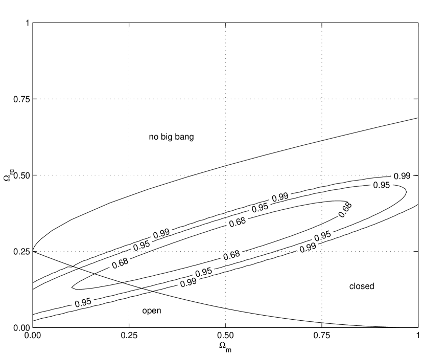
Figure 1: The probability distribution function for the parameters $\Omega_{m}$ and $\Omega_{rc}$ in the DGP model, for the presently available dataset of 92 Type Ia supernovae—see the text for detailed description of the method. The $68\%$, $95\%$ and $99\%$ confidence contours in the $\Omega_{rc}-\Omega_{m}$ plane are shown, as well as the line separating closed universes with big bang from no-big-bang ‘bouncing’ ones and the one separating closed and open universes (ie, denoting the flat ones).

The normalized PDF is obtained by dividing the above expression by its sum over all possible values of the parameters s. In the particular case of our model the cosmological parameters are $H_{0}$, $\Omega_{m}$ and $\Omega_{rc}$. The probability distribution function for the parameters $\Omega_{m}$ and $\Omega_{rc}$ is obtained by integrating over all possible values of $H_{0}$, and the results are displayed in Fig. 1.

We have also studied the improvements in the parameter estimation using supernovae which are expected from future studies of cosmic acceleration. Following (Weller & Albrecht, 2001) we assumed a future dataset similar to one proposed for the SNAP satellite. This has the magnitudes of 50, 1800, 50 and 15 supernovae in the red-shift ranges from $z=0-0.2$, $z=0.2-1.2$, $z=1.2-1.4$ and $z=1.4-1.7$ respectively. The statistical error in magnitude is assumed to be $\sigma=0.15$ including both the estimated measurement error of the distance modulus and the dispersion in the distance modulus due to the dispersion in galaxy redshift. The supernovae dataset was generated assuming that we live in a standard FRW universe with cosmological parameters $\Omega_{m}=0.3$ and $\Omega_{\Lambda}=0.7$. Fig. 2 shows the corresponding results.

4 Results and Discussion

A number of interesting features are apparent from Fig. 1. Firstly, the likelihood analysis of the supernovae data is degenerate in the $\Omega_{rc}-\Omega_{m}$ plane, approximately following a line of the form

$$\Omega_{rc}\sim\frac{2}{5}\Omega_{m}+\frac{1}{10}\,.$$ (20)

This is to be compared with the standard cosmological scenario, where the degeneracy is approximately along

$$\Omega_{\Lambda}\sim\frac{4}{3}\Omega_{m}+\frac{1}{3}\,.$$ (21)

Hence one can say that for any given value of $\Omega_{m}$, the value of $\Omega_{rc}$ which provides the best-fit to the supernova data is always lower than the corresponding value of $\Omega_{\Lambda}$. Reversing the argument, one could also say that for a given value of the density of the accelerating component (a cosmological constant in the standard case or the bulk-induced term in the DGP model) the DGP model requires a higher matter density in order to fit the supernova data. Note that the two and three sigma likelihood contours are quite close to each other, and relatively distant from the one sigma contour. This indicates that with the currently available data there is an elongated ‘degenerate best-fit plateau’, and beyond this plateau the likelihood drops quite abruptly.

In any case, just by looking at Fig. 1 one might think that there is a rather comfortable range of matter densities which would give models in agreement with observation. However this is not the case as there are other cosmological constraints that must be met. In particular, the most recent CMB data (de Bernardis et al., 2000; Lange et al., 2001; Netterfield et al., 2001; Hanany et al., 2000; Balbi et al., 2000; Stompor et al., 2001; Halverson et al., 2001; Pryke et al., 2001) gives a strong indication that the universe is spatially flat or very nearly so. The current constraint is

$$\Omega_{tot}=1.00\pm 0.05\,;$$ (22)

note that only fairly weak priors are needed to derive this constraint (refer to the original CMB papers for the analysis details). Combining this with the supernova analysis this leaves a much smaller range of allowed models. At the $68\%$ confidence level, the allowed range of matter densities is approximately

$$\Omega_{m}=0.20\pm 0.05\,,$$ (23)

while at the $99\%$ confidence level it is

$$\Omega_{m}=0.2\pm 0.1\,.$$ (24)

Note that this result is quite robust—for example, we have checked that it is unchanged if the likelihood analysis is restricted ab initio to flat universes.

The final piece of observational evidence that we shall use are dynamical measurements of the total mass density—see Turner (2000a, b) for a discussion of the state-of-the-art. In particular the ratio of baryons to the total mass in clusters has been determined using both X-ray measurements (Mohr et al., 1999) and Sunyaev-Zel’dovich measurements (Carlstrom et al., 1999). One respectively obtains

$$f_{x}=(0.075\pm 0.007)h^{-3/2}\,$$ (25)

from X-ray measurements, and

$$f_{sz}=(0.079\pm 0.010)h^{-1}\,$$ (26)

from the Sunyaev-Zel’dovich effect. In both cases, various dozens of sources have been used in the analysis. If one assumes that clusters are a fair sample of the matter content of the universe (which is very reasonable given their large size) and uses the latest value of the baryon density at nucleosynthesis (Burles, Nollett & Turner, 2000)

$$\Omega_{b}=(0.020\pm 0.002)h^{-2}\,,$$ (27)

together with the value of the (re-scaled) Hubble constant $h$ obtained by the HST Key Project (Freedman et al., 2000),

$$h=0.72\pm 0.08\,,$$ (28)

one finally obtains the (rather conservative) estimate

$$\Omega_{m}=0.35\pm 0.07\,.$$ (29)

More recently, there have been claims of an even narrower (though perhaps slightly optimistic) range (Turner, 2001) at the one sigma level

$$\Omega_{m}=0.330\pm 0.035\,.$$ (30)

Note also that there are various other sources of supporting evidence that are consistent with the above value, including studies of the evolution of cluster abundances with redshift, measurements of the power spectrum of large-scale structure (such as the recent preliminary 2dF results (Percival et al., 2001)), analyses of measured peculiar velocities as they relate to the observed matter distribution, and observations of the outflow of material from voids. A discussion of the assumptions and techniques of each method can be found in Turner (2000a, b).

Hence the DGP model’s proposal for the acceleration of the universe requires a value of the matter density that is inconsistent, at least at the two sigma level, with the observationally estimated matter density of the universe. Together with the fact that gravity becomes weaker on large enough scales, this presents a serious problem. Note that if the required mass was larger than the standard case, one could perhaps argue that there was some matter in an yet undetected form. Indeed, the fact that in the DGP model gravity becomes weaker on large enough scales could then be used to obtain a relatively simple explanation. However, since the observationally acceptable range of masses is lower than the standard model, no explanation of this kind is possible. In any case, one should recall that the evolution of the universe should be as standard in the DGP model up to very recent times, eg in what concerns the Friedmann equation for example—which also places strong constraints on any attempts to ‘get rid of’ some of the matter.

And finally, there is yet another hurdle for this model to overcome. In (12) we derived the redshift at which the universe switches from deceleration to acceleration, for the case of a flat universe. We plot this redshift, for the range of matter densities given by (24), in Fig. 3, together with the analogous curve for the standard model. The problem is now apparent: for the specified range of matter densities, the redshift of turnaround decreases as the matter density increases. On the other hand, for a given value of the turnaround redshift, the required matter density is always lower with a bulk-induced term replacing a cosmological constant (the solid curve in Fig. 3) than in the standard model with a cosmological constant (the dashed curve). Now, the latest supernova data (Perlmutter et al., 1997, 1999; Riess et al., 1998, 2001; Turner & Riess, 2001; Avelino, de Carvalho & Martins, 2001) indicates that the universe switched from deceleration to acceleration at a redshift in the interval (at one-sigma level)

$$0.6<z_{q=0}<1.7\,.$$ (31)

Note that for values of the matter density close to the upper limit $\Omega_{m}\sim 0.3$ the predicted redshift of turnaround is already smaller than this range.

This, therefore, is the dilemma of these models. On the assumption of a flat universe, a very low matter density is needed so that acceleration starts early enough. This is in fact confirmed by the simulation of the supernova analysis for a SNAP-class dataset, which is shown in Fig. 2: closed models are still favoured, though flat ones are still possible at around the two sigma level. However the range of possible matter densities is significantly reduced. Note that in generating the SNAP dataset we have assumed a standard FRW universe with $\Omega_{m}=0.3$ and $\Omega_{\Lambda}=0.7$. Hence, according to our discussion above, if we fit that dataset to the accelerating DGP model then the preferred value of the matter density will come out lower. This is a trivial consequence of the fact that the type Ia supernova analysis method is basically a cosmological ‘accelerometer’. The point is that, even with the data available today, such low values are already strongly disfavoured by dynamical measurements of the total mass density in the universe.

On the other hand, even if one would be willing to admit that such values were allowed on the grounds of dynamical measurements alone (implying a much smaller value of dark matter than in the standard model), they are expected to run into serious difficulties when it comes to density fluctuation growth and the evolution of large-scale structures (which can now be probed much beyond Mpc scales both by direct surveys and through gravitational lensing), again because of the weaker gravity on large enough scales. For the DGP scenario to be viable the characteristic scale would be of order $r_{c}\sim H_{0}^{-1}$, but obviously the effects of weaker gravity would be felt on smaller scales than this. Indeed this point has already been made on rather general grounds (though only for the case of sub-horizon modes) by Uzan & Bernardeau (2000), and we shall return to it in more detail elsewhere.

5 Conclusions

In this paper we have considered the cosmological consequences of the brane world model of Dvali, Gabadadze & Porrati (2000), and its proposed alternative explanation for the current acceleration of the universe. We have shown that, contrary to recent claims (Deffayet, Dvali & Gabadadze, 2001), this proposal is already strongly disfavoured by existing cosmological datasets, at least at the two sigma level. In order to be consistent with CMB and supernova data one would need a very low matter density $\Omega_{m}\sim 0.2$. Even if this was allowed by dynamical measurements (such as cluster data), such a low density ( and hence such a small amount of dark matter) together with the fact that gravity is weaker on large enough scales would make it difficult to produce a consistent structure formation scenario.

The lesson to be learned from this exercise is twofold. Firstly, no matter how interesting or mathematically clever one’s favourite particle physics model of the universe might be, the first hurdle towards credibility consists in deriving falsifiable cosmological predictions from it. And secondly, the currently available cosmological observations are already powerful enough to impose tight constraints on a wide range of possible models, especially when various cosmological datasets are combined—which is a sign that the era of precision cosmology has indeed started. We hope that other brane world scenarios can be brought into the realm of cosmological testability in the near future.

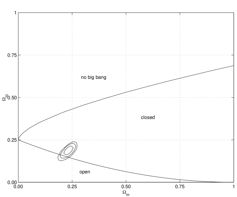
Figure 2: A simulation of the analysis with a SNAP-class dataset generated assuming that we live in a standard FRW universe with cosmological parameters $\Omega_{m}=0.3$ and $\Omega_{\Lambda}=0.7$—see the text for the other assumptions involved. Contours and boundary lines are as in Fig. 1.

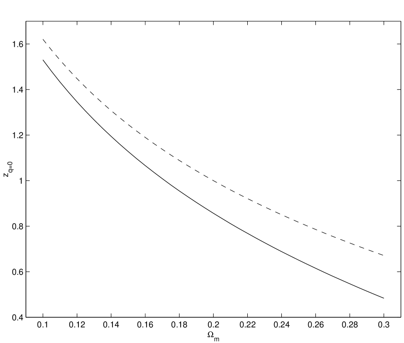
Figure 3: The redshift of ‘turnaround’ for which the deceleration parameter vanishes, as a function of the matter density in the DGP models, for the values of the matter density that are consistent (up to $99\%$ confidence level) with type Ia supernova and CMB data (solid line), and the analogous quantity in the standard cosmological model (dashed line). In both cases $\Omega_{tot}=1$.

References

- Arkani-Hamed, Dimopoulos & Dvali (1998) Arkani-Hamed, N., Dimopoulos, S., and Dvali, G. 1998, Phys. Lett. B429, 263
- Avelino, de Carvalho & Martins (2001) Avelino, P.P., de Carvalho, J.P.M., and Martins, C.J.A.P. 2001, Phys. Rev. D, in press (see astro-ph/0103075)
- Balbi et al. (2000) Balbi, A. et al. 2001, ApJ545, 5
- Behnke et al. (2001) Behnke, D., Blaschke, D., Pervushin, V.N., and Proskurin, D. 2001, gr-qc/0102039
- Binétruy et al. (2000) Binétruy, P., Deffayet, C., Ellwanger, U., and Langlois, D. 2000, Phys. Lett. B477, 285
- Burles, Nollett & Turner (2000) Burles, S., Nollett, K.M., and Turner, M.S. 2000, astro-ph/0010171
- Carlstrom et al. (1999) Carlstrom, J. et al. 1999, astro-ph/9905255
- de Bernardis et al. (2000) de Bernardis, P. et al. 2000, Nature 404, 955
- Deffayet (2001) Deffayet, C. 2001, Phys. Lett. B502, 199
- Deffayet, Dvali & Gabadadze (2001) Deffayet, C., Dvali, G., and Gabadadze, G. 2001, astro-ph/0105068
- Dev, Sethi & Lohiya (2000) Dev, A., Sethi, M., and Lohiya, D. 2000, astro-ph/0008193
- Dick (2001) Dick, R. 2001, hep-th/0105320
- Dvali, Gabadadze & Porrati (2000) Dvali, G., Gabadadze, G., and M. Porrati, M. 2000, Phys. Lett. B485, 208
- Freedman et al. (2000) Freedman, W.L. et al. 2000, astro-ph/0012376
- Halverson et al. (2001) Halverson, N.W. et al. 2001, astro-ph/0104489
- Hanany et al. (2000) Hanany, S. et al. 2001, ApJ545, 1
- Lange et al. (2001) Lange, A.E. et al. 2001, Phys. Rev. D63, 042001
- Maartens (2001) Maartens, R. 2001, gr-qc/0101059
- Mannheim (2001) Mannheim, P. 2001, astro-ph/0104022
- Mohr et al. (1999) Mohr, J. et al. 1999, ApJ517, 627
- Netterfield et al. (2001) Netterfield, C.B. et al. 2001, astro-ph/0104460
- Percival et al. (2001) Percival, W.J. et al. 20001, astro-ph/0105232
- Perlmutter et al. (1997) Perlmutter, S. et al. 1997, ApJ483, 565
- Perlmutter et al. (1999) Perlmutter, S. et al. 1999, ApJ517, 565
- Pryke et al. (2001) Pryke, C. et al. 2001, astro-ph/0104490
- Randall & Sundrum (1999) Randall, L., and Sundrum, R. 1999, Phys. Rev. Lett. 83, 3370
- Riess et al. (1998) Riess, A. et al. 1998, AJ116, 1009
- Riess et al. (2001) Riess, A.G. et al. 2001, astro-ph/0104455
- Rubakov (2001) Rubakov, V. 2001, hep-ph/0104152
- Stompor et al. (2001) Stompor, R. et al. 2001, astro-ph/0105062
- Turner (2000a) Turner, M.S. 2000, Physica Scripta T85, 210
- Turner (2000b) Turner, M.S. 2000, Physics Reports 333, 619
- Turner (2001) Turner, M.S. 2001, astro-ph/0106035
- Turner & Riess (2001) Turner, M.S., and Riess, A.G. 2001, astro-ph/0106051
- Uzan & Bernardeau (2000) Uzan, J.-P., and Bernardeau, F. 2000, hep-th/0012011
- Wang & Garnavich (2001) Wang, Y., and Garnavich, P. 2001, ApJ552, 445
- Wang et al. (2000) Wang, Y. et al. 2000, ApJ536, 531
- Weller & Albrecht (2001) Weller, J., and Albrecht, A. 2001, Phys. Rev. Lett. 86, 1939