11email: M.H.vanKerkwijk@astro.uu.nl 22institutetext: Palomar Observatory, California Institute of Technology 105-24, Pasadena, CA 91125, USA
22email: srk@astro.caltech.edu
Optical spectroscopy and photometry of the neutron star
RX J1856.5$-$3754††thanks: Based on observations collected at the European
Southern Observatory, Paranal, Chile (ESO Programmes 63.H-0416
and 65.H-0643).
We present spectroscopy and imaging with the Very Large Telescope (VLT) of the neutron star RX J1856.5$-$3754. Little is known about the nature of this source other than that it is a nearby hot neutron star. Our VLT spectrum does not show any strong emission or absorption features. With considerable care to photometric calibration, we obtain photometric measurements over the optical and ultra-violet (UV) using our VLT observations and a detailed analysis of archival Hubble Space Telescope data. We find that the entire optical to UV spectral energy distribution is well described by a slightly reddened Rayleigh-Jeans tail (, where is the reddening curve; implied ). The reddening is consistent with the interstellar absorption inferred from X-ray spectroscopy. The simplest explanation for this Rayleigh-Jeans emission is that the optical-UV radiation arises from thermal emission from the surface of the neutron star. The high degree to which the data conform to the Rayleigh-Jeans tail significantly limits contributions from other sources of emission. In particular, our observations are inconsistent with the presence of an accretion disk and also strongly constrain the amount of magnetospheric emission from this enigmatic neutron star.
Key Words.:
stars: individual (RX J1856.5$-$3754) — stars: neutron – X-rays: stars1 Introduction
The soft X-ray source RX J1856.5$-$3754 is the brightest and nearest of the so-called isolated neutron stars111Given that most radio pulsars are also isolated, a better name might be ‘thermally emitting’ neutron stars. (for a review, see Treves et al. 2000). These objects have X-ray spectra which appear to be entirely thermal, indicating that the emission arises from the photosphere and that there is little if any contamination from ill-understood emission processes such as those occurring in magnetospheres in radio pulsars and accretion flows in X-ray binaries. Therefore, these objects offer perhaps the best hope of modeling neutron-star spectra, and inferring the effective temperature, surface gravity, and gravitational redshift. In principle, this could lead to unique constraints on the equation of state of matter in the neutron star interiors (e.g., Lattimer & Prakash 2001).
Given these possible gains, ever since its discovery in 1996 by Walter et al., RX J1856.5$-$3754 has been the subject of much observational attention. Walter & Matthews (1997) used the Hubble Space Telescope (HST) to discover a very faint, , optical counterpart; its flux is roughly consistent with seeing the Rayleigh-Jeans tail of the spectrum. Further HST observations were used by Walter (2001) to measure the parallax, while Pons et al. (2001) used HST, ROSAT, ASCA, and EUVE to measure the broad-band spectral energy distribution.
Pons et al. (2001) also presented detailed model atmospheres for a variety of compositions, with which they were able to model the broad-band spectrum satisfactorily. This leads to strong constraints on the temperature. When combined with the parallax, however, the inferred radii are too small for realistic neutron star models. Pons et al. suggest the surface may not have a uniform temperature distribution. If so, the broad-band spectrum can be used to set only weak constraints on the equation of state.
If one could observe spectral features in the spectrum, one might be able to measure the surface gravity and gravitational redshift without much ambiguity (Paerels 1997). In this respect, the first spectrum at good resolution, taken with XMM of RX J0720.43125, was disappointing, as no features were seen (Paerels et al. 2001). Recent results on RX J1856.5$-$3754 appear similarly disappointing, with neither X-ray spectra taken with Chandra (Burwitz et al. 2001), nor ultra-violet spectra taken with HST (Pons et al. 2001) showing strong features.
The use of RX J1856.5$-$3754 to address the fundamental issues in physics and astrophysics mentioned above would benefit from – or even require – understanding the nature of the source. Walter et al. (1996) suggested it could be a young, cooling neutron star, or a neutron star kept hot by accretion from the interstellar medium. An alternative would be that it is a few million-year old magnetar, as was suggested for RX~J0720.4$-$3125 on the basis of its 8.4-s periodicity (Kulkarni & van Kerkwijk 1998). An indication that RX J1856.5$-$3754 might be young is its proper motion, which Walter (2001) found to point away from the nearby Sco-Cen association. This has led him to the plausible suggestion that RX J1856.5$-$3754 was born in this association about a million years ago. For a young neutron star, however, it is hard to understand the lack of X-ray pulsations. Could it be that this neutron star has no significant magnetic field? Almost certainly, the interpretation of the high resolution X-ray spectra of this source will depend on knowing the composition of the atmosphere, the strength of the magnetic field, and the level of non-thermal emission.
| Objecta | UTb | Slit or | Par.c | |||
|---|---|---|---|---|---|---|
| day, time | Filter | (s) | (°) | |||
| EG 274 | 15, | 23 02 | 5″ | d | 1.21 | |
| X-F/ | 23 58 | B | 300 | 1.67 | ||
| 16, | 00 08 | 1″ | 2700 | 1.60 | ||
| 00 58 | B | 1.33 | ||||
| 01 17 | 1″ | 1.26 | ||||
| 02 54 | 5″ | 300 | 1.06 | |||
| X-L/ | 03 11 | 1″ | 1.05 | |||
| 04 45 | 5″ | 300 | 1.04 | |||
| X-F/ | 05 00 | 1″ | e | |||
| X-F/ | 06 06 | 1″ | 1.15 | |||
| 07 56 | 5″ | 300 | 1.57 | |||
| BPM 16274 | 08 08 | 5″ | d | 1.21 | ||
| 10 36 | 5″ | d | 1.14 | |||
a X-F and X-L are exposures taken at the indicated position
angle, for which the slit passes over RX J1856.5$-$3754 and star F or L (see
Fig. 1); standards were taken at position
angle .
b UT day in July 1999.
c Parallactic angle at start of observation.
d Third exposure taken with a GG 435 order separation filter.
e Lost because of a glitch in telescope pointing.
In an effort to understand the nature of this important but enigmatic source, we have undertaken a series of observations. In this paper, we report on the first optical spectrum of RX J1856.5$-$3754 and on accurate optical-UV photometry. In our spectra, we find evidence for a nebula around RX J1856.5$-$3754. Those observations and the interpretation of the nebula will be the subject of the next paper (Van Kerkwijk & Kulkarni, in preparation).
The organisation of this paper is as follows. We describe our observations in Sects. 2 and 3, and the reduction in Sect. 4. We pay particular attention to accurate calibration, since some of our results turn out to be discrepant with previously published ground-based results. We also re-analyse the HST imaging, taking particular care to correct for systematic effects affecting faint stars. We discuss the results in Sects. 5 and 6.
2 Spectroscopic observations
We observed RX J1856.5$-$3754 on the night of 1999 July 15 to 16 at the 8-m Unit Telescope #1 (Antu) of the Very Large Telescope at Paranal, using the Focal Reducer/Low Dispersion Spectrograph FORS1 to obtain spectra covering the optical range and a number of images. A log of the observations is given in Table 1. The conditions were good, with the seeing varying from to . The night started with patchy high cirrus, which disappeared later. The spectroscopy was done using a grism, the standard resolution collimator (final f-ratio of 3.13), and a Tektronix CCD detector with pixels of . With this setup, the plate scale is , and the 3600–9000 Å wavelength range is covered at . With the 1″ slit, the wavelength resolution is . The detector was read out through all four amplifiers, using the high gain setting () for the spectra, and the low gain setting () for the images.
| Objecta | UTb | Sequencec | Seeing | ||
|---|---|---|---|---|---|
| day, time | (″) | ||||
| RX J1856 | 1, | 06:57–07:52 | BRRR | 1.14–1.06 | |
| 07:54–08:48 | BRRR | 1.05–1.02 | |||
| RX J1856 | 2, | 07:23–08:16 | BRRR | 1.09–1.04 | |
| 08:19–09:11 | BRRR | 1.03–1.02 | |||
| 09:14–09:45 | BRR | 1.03–1.04 | |||
| PG 0942 | 2, | 23:10–23:20 | BRBR | 1.08 | |
| RX J1856 | 3, | 06:00–06:54 | BRRR | 1.27–1.13 | |
| 06:59–07:51 | BRRR | 1.12–1.05 | |||
| 08:00–08:52 | BRRR | 1.04–1.02 | |||
| PG 1657 | 09:26–09:51 | BRBR | 1.60–1.69 | ||
| 09:54–10:05 | BRBR | 1.71–1.81 | |||
| RX J1856 | 4, | 06:25–07:18 | BRRR | 1.19–1.09 | |
| 07:23–08:16 | BRRR | 1.08–1.03 | |||
a In full: RX J1856.5$-$3754, PG 0942$-$029 and
PG 1657+078.
b UT day in May 2000.
c For RX J1856.5$-$3754, the integration times were 138 s in B, 135 s in
R, and 1019 s in H; for the standards, 3 and 20 s in B, and 1
and 20 s in R.
d The B-band image has seeing.
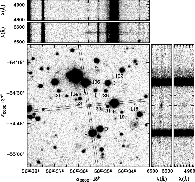
Since the source is faint, we set up using two brighter stars nearby, stars F and L (here and below we follow the nomenclature of Walter et al. [1996]; see also Fig. 1), chosing the position angle such that the counterpart of RX J1856.5$-$3754 (hereafter star X) should fall in the slit as well. To measure the positions, we reanalysed the images of Walter & Matthews (1997), taken through F606W and F300W filters with the Wide Field Planetary Camera 2 (WFPC2) on board HST. The analysis of the HST images is described in more detail in Sect. 4.6.
In order to minimise slit losses due to differential refraction, we took set-up images through a Bessel B filter, used the differential refraction corrector of FORS1, and chose as reference the star for which the position angle was closest to the parallactic one. We obtained spectra with a total exposure time of 6.5 hour, taking individual exposures at various positions along the slit in order to mitigate the effect of bad pixels and other defects. To calibrate the slit losses, we followed our sequences of long integrations with short exposures through a wide slit (5″, formed using the multi-object slitlets). We observed two spectrophotometric flux standards through the wide slit to calibrate the instrumental response.
For verification of our set-up, we took a 5-minute B-band image before starting the first spectroscopic observation (which used star F as reference). From the image, star X appeared to have moved to the East.222In the meantime, the proper motion has been measured accurately using HST (Walter 2001). After the first spectrum, therefore, we took three additional 5-minute B-band images333Photometry of star X using these images was presented by Neuhäuser (2001). He finds , consistent with (though substantially less accurate than) our result. to measure a more accurate position, and found that star X had, rather fortuitously, moved exactly along the slit; hence, the first spectrum was not lost. For star F, we therefore kept the same set-up, while we changed the position angle for star L appropriately.
3 B, R, and H imaging
Images in B, R, and H of RX J1856.5$-$3754 and its environment were taken for us in the nights of 2000 April 30, May 1, May 2, and May 3, at Unit Telescope #2 (Kueyen) using the Focal Reducer/Low Dispersion Spectrograph FORS2. The standard resolution collimator was used, and a Tektronix CCD detector with pixels of . The corresponding plate scale is .
During all nights the seeing was good, varying between 055 and 08. The nights of 2000 May 1 and May 2 were photometric, the night of April 30 mostly clear. Clouds appeared during the second half of the night of May 3, which includes the time used for RX J1856.5$-$3754; from the count rates, however, it appears that the clouds did not affect the observations. In total, ten series of images were taken of RX J1856.5$-$3754 (see Table 2). Nine were in the order B, R, H, R, H, R, and one – used to fill up time – was shortened to B, R, H, R. Of the latter, the B-band image has much worse seeing and is not used. The total exposure time is about 21 minutes in B, 1 hour in R, and 5 hours in H. During the photometric night, several standard fields of Landolt (1992) were observed. No useful separate H calibration images were taken.
4 Reduction
The data were reduced using the Munich Image Data Analysis System (MIDAS) and procedures running in the MIDAS environment. From bias frames taken before and after a given night, the bias level appeared somewhat variable, both in time and in position on the detector. However, relative to the levels found from the overscan pixels (determined separately for the four amplifiers), it remained constant. For bias subtraction, therefore, we subtracted both the levels from the overscan regions in individual frames and an average of the overscan-corrected bias frames (for the appropriate gain setting). The averages were determined separately for 1999 and 2000.
4.1 Photometry
All images were corrected for sensitivity variations using flat fields constructed from images of the sky taken at dusk and dawn (for the observations in 2000, only the dawn frames were used, since this produced much cleaner results). Averages were formed of the various series after filtering out cosmic-ray hits, verifying that even for the best-seeing images no stars were mistakenly affected.
Photometry was done by first determining the offset of instrumental magnitudes derived from the average frames from those derived from the images of the first sequence in the night of 2000 May 2, and then applying a calibration determined from the three standard fields observed during that night. We measured instrumental magnitudes using the DAOphot package (Stetson 1987). We used an iterative procedure, in which relatively isolated stars were selected and used to define a point-spread function (PSF), next the PSF was used to fit all stars and to subtract all but the PSF stars, and then the cleaned frame was used to determined an improved PSF, etc. We found that to model the variations in the PSF over the frame, a second-order dependence on position was required. Aperture corrections were determined from the difference between the fitted magnitudes and magnitudes measured in 20-pixel (4″) radius apertures on the PSF stars in the final frame in which all non-PSF stars had been removed.
The standard fields were analysed in two separate ways. For deriving the calibration using the Landolt (1992) photometry, we simply determined appropriate aperture magnitudes on the reduced frames (if not overexposed; in practice, we could only use the short frames). We inferred extinction coefficients of 0.126 and 0.076 in B and R, respectively, which are smaller than the typical values of 0.21 and 0.13 listed by ESO. We did not have sufficient data to measure the colour terms accurately, although we could confirm that the colour term for the B band is significant (, i.e., the ESO B band is bluer than Landolt B), while the colour term for the R band is negligible. We estimate that the final uncertainty in the zero points is about 0.02.
We also tried to calibrate our fields using fainter stars, since for many faint stars in Landolt fields, Stetson (2000) has obtained calibrated magnitudes from archive observations. For this purpose, we analysed the frames using point–spread function fitting as described above. Unfortunately, however, while for the field of PG 1657+078, there are 32 stars with B-band magnitudes and 44 with R, for the field of PG 0942029 there is only one star. As a result, we cannot derive an accurate solution including extinction terms, but only confirm the solution found using the Landolt photometry.
In Table 5, we list photometry for all point-like objects which are present in the HST Planetary Camera images taken through the F606W filter (Walter et al. 1996; Walter 2001), and which are detected in both and . One word of caution about the brightest stars, with , which are overexposed in many of the R-band images. The magnitudes of these stars have been determined by PSF fitting to those pixels which were not overexposed, and are therefore somewhat more uncertain. We compared the magnitudes for these stars with magnitudes inferred from the first series of images, in which overexposure is less of an issue because of the relatively bad seeing. We found that the photometry in Table 5 may slightly underestimate the true brightness of the stars, by .
4.2 Spectroscopy
For the spectroscopy, the flat fielding turned out to be problematic, because the spectroscopic flats, taken with the internal flat-field lamp illuminating the instrument cover, had an illumination pattern so different from that of the actual observations on sky that they were useless. Since the observations of the flux standards indicated that fringing was not a problem and that pixel-to-pixel sensitivity variations were much smaller than the sky-subtraction uncertainties for our very faint source, we decided to forego flat-fielding altogether. In order to equalise the four quadrants of the chip, which are read out through amplifiers with slightly different gain, we multiplied with the gains for the different amplifiers as measured by the instrument team. This provided very satisfactory results.
For the sky subtraction, clean regions along the slit within about 100 pixels of the sources of interest were selected, and these were fitted using a polynomial function. The order of the polynomial was mostly zero, but could be increased up to quadratic at any given column as long as further terms increased the goodness of the fit to the sky regions significantly. For each set of observations, the sky-subtracted images were registered and added together.
From both the individual and the summed sky-subtracted images, spectra were extracted using an optimal weighting scheme similar to that of Horne (1986). For this purpose, the spatial profile of the bright star (either F or L) was determined, and this was used to extract optimally weighted spectra at the position of the bright star itself, as well as at the position of star X. Furthermore, for verification, spectra were extracted at a number of empty positions. These were all consistent with zero flux.
The dispersion relation was found using an exposure of helium, argon and mercury lamps. Line positions were determined for positions along the whole slit. At a single position, a fourth order fit was sufficient, giving root-mean-square residuals of 0.5 Å; to obtain the same residuals for a two-dimensional relation required terms up to fifth order along the dispersion direction and second order along the spatial direction (for a total of 18 terms). The latter solution was used to calculate the wavelengths for all extracted spectra.
4.3 Spectral Images
In the extracted spectra of RX J1856.5$-$3754, emission lines of H and H appeared. Inspection of the sky-subtracted frames showed that these lines were extended, especially along the slit over star F. In fact, it extended into the regions used to define the sky emission, and hence it had been partly removed in the sky-subtraction stage. In order to provide a cleaner picture, we rebinned the raw images to spectral images, in which every column is at a constant wavelength, removed cosmic rays, and formed averages for the two slit positions (excluding the first spectrum, which had a cosmic-ray hit at H near the target). Next, we determined the sky emission as a function of wavelength in regions far away from the neutron star, and subtracted this from all columns. The parts of the images around H and H are shown in Fig. 1. From these spectral images, it is already clear that the neutron star has a nebula which is extended along the path it has travelled. This is confirmed by our H imaging. The H images and a discussion of the nature of this nebula will be presented elsewhere (Van Kerkwijk & Kulkarni, in preparation).
4.4 Flux calibration of the spectra
For the flux calibration, the spectra were first corrected for atmospheric extinction using the average La Silla extinction curve. While this will be only approximately correct, it facilitates the next step, the determination of the slit losses. For this purpose, the ratio with the wide-slit spectra was formed for each of the bright star spectra taken through the 1″ slit. These ratio spectra were approximated with second-degree polynomials, which were used to correct all spectra.
Finally, the spectra were corrected for the response of the spectrograph derived from the observation of the spectrophotometric standard EG~274 (Hamuy et al. 1992, 1994). The spectra of this standard were extracted in the same manner as described above, but in addition a correction was made for the blue second-order light that overlaps the part of the spectrum at (the correction was determined with the help of the spectrum taken through the GG 435 filter). We observed the DA white dwarf BPM~16274 as an additional calibrator. Unfortunately, we realised later that this star is only calibrated in the ultraviolet. We still used it to verify our response curve using a model spectrum kindly provided by D. Koester (for and , as inferred by Bragaglia et al. [1995], and normalised to , as measured by Eggen [1969]). For wavelengths longer than , the comparison was very satisfactory, as was a similar comparison using a DA white-dwarf model provided by D. Koester for EG~274 (, ; Vauclair et al. 1997).
The above gives us confidence that the relative calibration over the spectral range is accurate. The accuracy of the absolute calibration, however, is less clear, since the spectra of EG~274 were taken in the beginning of the night, when some patchy cirrus was still present. In order to assess the influence of the cirrus, we compared fluxes from all B-band (acquisition) images and all wide-slit spectra. We found that there were variations before about 1 ut, but that after that time the measured count rates indicate the sky was clear. To see whether our flux calibration was influenced by the cirrus, we used the B, V, and R filter curves of Bessell (1990) to determine synthetic B, V, and R-band magnitudes for all brighter objects in our wide-slit spectra. For BPM~16274, we find , , quite consistent with the observed , (Eggen 1969). Also for stars F (twice), L, and C (in the slit for the star L position; see Fig. 1), the synthetic magnitudes are in good agreement with our B and R-band photometry, as can be seen in Table 3. We conclude that the absolute calibration of our spectra is accurate to 0.02.
4.5 Previous photometry of stars L, C, and F
While our spectrophotometry of stars L, C, and F agrees well with our own photometry, it disagrees with measurements in the literature: the synthetic V-band magnitudes are 0.4 brighter than both the V-band magnitudes of Neuhäuser et al. (1997) and the V-band magnitudes inferred from Gunn g and r measurements of Campana et al. (1997). (The magnitudes of Walter et al. (1996) differ even more, by , but Neuhäuser et al. have already noted that Walter et al. used an incorrect zero point.)
Comparing colours, we find that our synthetic and colours are systematically redder and bluer, respectively, than those of Neuhäuser et al. (1997). The inferred values, however, are consistent. This suggests there may be a problem with the V-band only. Indeed, the V, , and values listed by Neuhäuser et al. imply B and R-band magnitudes that are in reasonable agreement with our values for bright stars like stars L, C, and F. If our synthetic B and R are correct, however, our synthetic V should be correct too, since the three bands are tied to each other by relative calibration on wide-slit spectra, which proved very reliable on BPM~16274.
In order to settle the issue, we classified the spectra (see Fig. 2), using the spectral atlases of Silva & Cornell (1992) and Torres-Dodgen & Weaver (1993). All three stars appear to be of spectral type G; see Table 3. For all three, our colours are consistent with the spectral types (for a small amount of reddening; see Sect. 5), while the and (but not ) colours of Neuhäuser et al. (1997) and the colour of Campana et al. (1997) are inconsistent with the spectral types (independent of reddening). We thus conclude that, despite the inconsistencies with earlier work, our calibration is reliable.
| Star | Spectral type | |||||
|---|---|---|---|---|---|---|
| L | G3–6 V–III | 0.64–0.66 | 0.36–0.37 | |||
| 18.07 | 0.74 | 17.33 | 0.41 | 16.92 | ||
| 18.06 | 16.93 | |||||
| C | G6–8 V–III | 0.66–0.76 | 0.37–0.44 | |||
| 18.56 | 0.78 | 17.78 | 0.43 | 17.35 | ||
| 18.53 | 17.34 | |||||
| F | G9–K0 V–III | 0.79–0.82 | 0.45–0.47 | |||
| 17.94 | 0.88 | 17.06 | 0.46 | 16.60 | ||
| 17.93 | 0.86 | 17.07 | 0.46 | 16.61 | ||
| 17.91 | 16.58 |
4.6 Archival HST imaging
RX J1856.5$-$3754 has been a regular target for WFPC2 observations with HST, both to measure broad-band photometry (Walter & Matthews 1997; Pons et al. 2001) and to determine the proper motion and parallax (Walter 2001). We reanalysed all images (see Table 4), both to provide a final verification of our flux calibration, and to extend the optical spectral energy distribution for RX J1856.5$-$3754 to shorter wavelengths. In our analysis, we take into account that during the last years updated zero points have become available (Baggett et al. 1997), and that new prescriptions have been published for correcting for changes in the amount of contaminants on the CCD windows (Baggett & Gonzaga 1998), for the so-called “long-versus-short anomaly” (Casertano & Mutchler 1998), and for the slowly degrading charge-transfer efficiency (CTE; Whitmore et al. 1999); the latter two are particularly important for faint objects. Furthermore, recently a package specifically written for WFPC2 photometry, HSTphot, has been made available by Dolphin (2000a), which includes many of the above corrections (Dolphin 2000b).

Our analysis started with the pipe-line reduced WFPC2 images. We measured photometry using HSTphot, as well as, for comparison, our own procedures. For the HSTphot reduction, we followed the prescription of Dolphin (2000a): (i) mask bad pixels; (ii) combine images taken at the same position and remove cosmic ray hits; (iii) determine sky levels; (iv) remove hot pixels; and (v) measure photometry by point-spread function fitting on the combined image(s). In the last step, we disabled the determination of point-spread function residuals and aperture corrections for the F170W image exposures, since these lack a sufficient number of well-exposed stars. For the F170W exposures, we also had to make a change to the source code for the sky determination, viz., to remove the constraint that the fitted sky level had to be positive. While this constraint is physically reasonable, slight inadequacies in the pipe-line subtraction of the bias and dark current can lead to negative count rates, which, if not corrected for, lead one to underestimate a source’s brightness; this is indeed the case for the F170W images. Another change we made to the source code was that we forced the use of the published (Dolphin 2000b) charge-transfer efficiency corrections for all bands (the multiphot routine in the HSTphot distribution uses more recent corrections for the optical filters, but not for the ultraviolet ones; the difference is rather small).
| Identifier | UT | Filter | |
|---|---|---|---|
| u3im010[1–4] | 1996 Oct 6 | F606W | |
| u3im010[5–6] | F300W | ||
| u51g010[1–8] | 1999 Mar 30 | F606W | |
| u51g030[1–4] | May 24 | F170W | |
| u51g040[1–8] | 26 | F450W | |
| u51g020[1–2] | Sep 16 | F300W | |
| u51g020[3–6] | F606W |
a u51g0106 has a high background and a large number of cosmic-ray hits. It has not been used in the analysis.
In Table 5, we list the results. For the F300W and F606W filters, the averages of the individual measurements are listed (no significant variability was found for any star). Comparing the HST photometry with our ground-based results, we find that the two are consistent.
To verify our technique, we also measured aperture photometry on averaged images, produced in the manner described by Van Kerkwijk et al. (2000). We measured count rates in apertures with a range of radii, derived aperture corrections to the standard 05 radius aperture, calculated the corrections discussed above (following the above references and the HST data and WFPC2 instrument handbooks), and converted to calibrated magnitudes by applying a 0.1 aperture correction from the 05 aperture to infinity and using the zero points of Baggett et al. (1997). We note that, as alluded to above, some corrections are large, especially for faint objects. For star X, the “long-vs-short” corrections are , , , and in F606W, F450W, F300W, and F170W, respectively (but see below); the 1996 CTE corrections are and in F606W and F300W, respectively; and the 1999 CTE corrections are , , , and in F606W, F450W, F300W, and F170W, respectively.
| Objecta | ||||||
|---|---|---|---|---|---|---|
| X | 21.37 0.10 | 23.00 0.07 | 25.19 0.07 | 25.21 0.06 | 25.64 0.02 | 25.80 0.11 |
| C | 21.62:: | 19.30 | 18.53 | 18.43 | 17.34 | |
| D | 20.80 | 19.28 | 19.07 | 17.69 | ||
| F | 20.70:: | 19.01 | 17.91 | 16.58 | ||
| I | 21.12 | 19.60 | 19.49 | 17.89 | ||
| J | 23.42:: | 21.83 | 21.64 | 20.39 | 20.08 | |
| L | 20.93:: | 18.72 | 18.06 | 16.93 | ||
| g | 20.74 | 20.48 | 20.44 | 19.72 | 19.48 | |
| 19 | 22.95 | 22.66 | 21.40 | 20.99 | ||
| 21 | 22.60 | 22.25 | 20.48 | 19.97 | ||
| 23 | 25.56:: | 24.97: | 23.26 | 22.68 | ||
| 24 | 21.98 | 21.62 | 19.80 | 19.34 | ||
| 26 | 22.28 | 22.19 | 20.90 | 20.56 | ||
| 28 | 23.10: | 22.16 | 21.93 | 21.05 | 20.79 | |
| 102 | 25.77:: | 25.37:: | 23.93 | 23.49 | ||
| 106 | 23.13 | 22.84 | 21.83 | 21.53 | ||
| 114 | 24.66: | 24.88: | 23.88 | 23.31 | ||
| 116 | 25.35:: | 23.55 | 23.05 | |||
| 1760 | 2955 | 4371 | 4520 | 5933 | 6464 | |
| 2.648 | 1.931 | 1.336 | 1.297 | 0.949 | 0.841 |
a X is the optical counterpart. For the other objects, the
nomenclature follows Walter et al. (1996, uppercase letters), Campana et al. (1997, two
digit numbers), Walter (2001, three-digit numbers) and
ourselves (object g). See Fig. 1.
b Magnitude differences between the ST and Vega systems.
These can be used to calculate the flux by
. From Baggett et al. (1997, WFPC2
filters) and Bessell et al. (1998, B and R).
c Effective wavelength and reddening for a Rayleigh-Jeans
() spectrum. See
App. A.
Comparing the results with those derived using HSTphot, we found good consistency for the brighter stars. For the fainter stars like star X, however, this was only the case if we did not apply the “long-versus-short” correction. Indeed, no such correction is applied in HSTphot, since Dolphin (2000b) has not found any evidence for it; he argues that its appearance likely reflects inaccurate sky subtraction in the procedures used by Casertano & Mutchler (1998). We do not have strong independent evidence either way, but note that if we do apply the correction, our VLT photometry for faint objects like star X becomes inconsistent with the HST results (while the results remain consistent for the brighter stars, since these are not affected).
Comparing to the magnitudes listed by Walter & Matthews (1997) and Walter (2001), we find that our results are roughly consistent for the brighter stars, but that they differ for the fainter stars; in particular, for star X, while the F606W magnitude is virtually identical, our F300W magnitude is 0.4 brighter than that of Walter & Matthews (note that these authors list magnitudes on the ST system). We suspect that the differences largely reflect our use of up-to-date corrections. This suspicion is strengthened by the fact that Pons et al. (2001), after making similar corrections, also find fluxes that differ from those of Walter & Matthews (1997). Indeed, their results are very similar to ours (their fluxes are fainter by and their uncertainties slightly larger, since they use aperture photometry rather than point-spread function fitting).
5 Spectrum and spectral energy distribution
The reduced, flux-calibrated spectrum is shown in Fig. 3. We limit ourselves to the wavelength range of 3800–7000 Å, since at shorter wavelengths the flux calibration becomes unreliable, while at longer wavelengths second-order light starts to contribute significantly for objects as blue as star X (it is negligible shortward of and rises approximately linearly to 10% at 7000 Å). We also removed 20 Å-wide regions around H, H, and H, which are (or might be in case of H) contaminated by nebular emission.
The spectrum does not contain any significant features. The best limits to the equivalent width of any feature are obtained shortward of : about 16 Å for features with 50% depth beneath the continuum, and about 60 Å for features with 25% depth.

The spectrum is shown together with the photometry in Fig. 4. One sees that the spectrum is consistent with both the VLT and HST photometry. Indeed, integrating the spectrum over the B and F450W bandpasses, we infer and , which compares well with our photometry (Table 5), giving additional confidence in the calibration of all three data sets.
Both spectrum and photometry indicate a spectral energy distribution close to that of a Rayleigh-Jeans tail, as would be expected for this very hot source. Assuming an intrinsic Rayleigh-Jeans spectrum, we determine the reddening to the source by fitting a reddened spectral distribution to the photometry. We do not include the spectrum in the fit, because we consider its absolute flux calibration somewhat less reliable and also because we wish to use it to verify the result from the photometry. We use the following relation between Vega magnitude and input spectrum ,
| (1) |
where is the response at wavelength , and is the magnitude difference between the Vega and ST systems (see Table 5). In the latter system, a flat spectrum has the same magnitude in all filters; it matches the Johnson system at V. The integrations are done over photon rates, since what we measure with CCDs is the rate of photons in a particular band. The response curves we used for the WFPC2 filters are the system response curves for the planetary camera, taken from the Space Telescope Science Institute web site. For the and filters, we used the Landolt filter curves from Bessell (1990). For the input spectrum, we take
| (2) |
where is the observed flux at reference wavelength and is the reddening. We use the reddening curve of Cardelli et al. (1989) for ; we include corrections for the optical as described by O’Donnell (1994). To minimise the covariance between and , we chose .
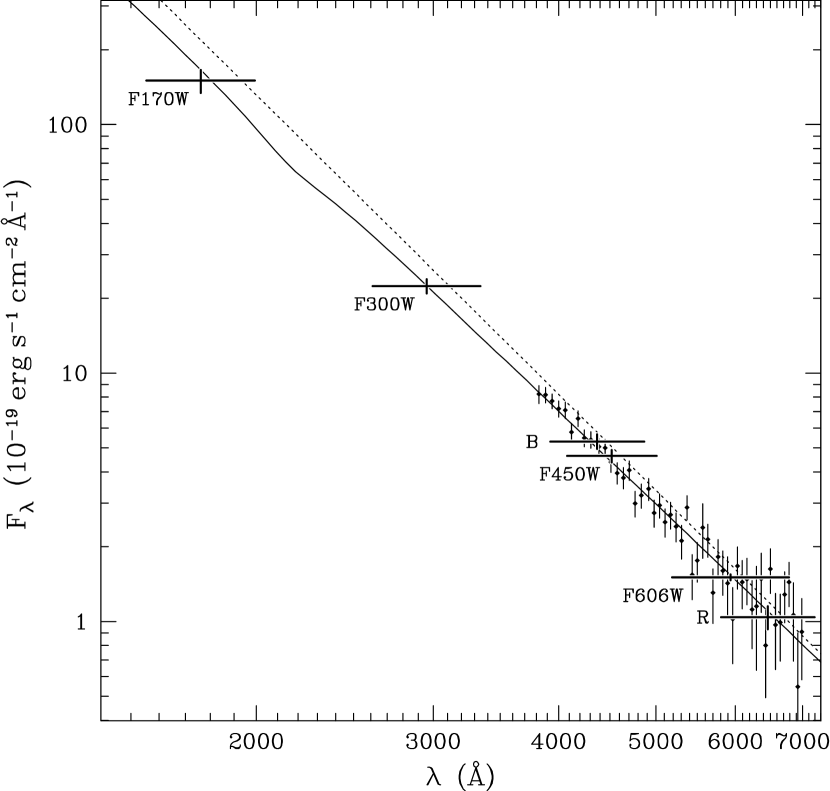
From the fit to the photometry, we find and ; the fit is acceptable, with for four degrees of freedom (six bands and two parameters; note that for the uncertainties we used the measurement errors with the zero-point uncertainties added in quadrature; see Table 5). For the reddening curve used, , and thus the unabsorbed flux is , where the error is dominated by the uncertainty in . The fit is shown in Fig. 4; it can be seen that it also is a good fit to the optical spectrum (see also Fig. 3), with for 49 degrees of freedom (no free parameters; also for other choices of binning, one finds ).
The inferred reddening is consistent with the range expected444We used , as inferred by Predehl & Schmitt (1995) for distant, highly absorbed objects. In these, the line of sight samples all phases of the interstellar medium; hence, the relation may not be valid locally. from the range in X-ray column density found from different model fits to the X-ray and EUVE spectrum (Pons et al. 2001; Burwitz et al. 2001). It is also consistent with the limit set by the total amount of reddening along this line of sight, which we can infer from stars L, C, and F. From the difference between the observed colours and the intrinsic colours for these stars (inferred from their spectral types; see Table 3), we infer , which corresponds to . Using this reddening, and assuming L, C, and F are main-sequence stars with absolute magnitudes , 5.4, and 5.8 (Cox 2000), respectively, their distances are 2.7, 2.8, and 1.6, respectively.555If they are giants, with (Cox 2000), they would be at and might be associated with the Sagittarius dwarf galaxy (Ibata et al. 1995), which is at and away from RX J1856.5$-$3754. Indeed, stars L and C have radial velocities of , consistent with being associated. Star F, with a radial velocity of , almost certainly is not associated. Thus, they are well in the background relative to star X, as well as relative to the CrA cloud complex, which, apparently, contributes very little extinction in this line of sight, unlike what was suggested previously (Walter et al. 1996).
6 Deviations from a Rayleigh-Jeans tail?
Above, we assumed a spectral energy distribution for star X. Indeed, from the observations, we cannot determine the slope of the spectrum independently: spectra with reproduce the photometry equally well as long as . However, stars L, C, and F pose an upper limit of 0.20 on the reddening to star X. Using , one infers that , i.e., the spectrum has to have a slope very close to that of a Rayleigh-Jeans tail.
6.1 Limits to a non-thermal component
Our data place stringent constraints on any contribution from non-thermal emission. For instance, fitting a sum of a Rayleigh-Jeans tail and a non-thermal spectrum with (i.e., ), such as observed for the Crab pulsar (Sollerman et al. 2000; Carramiñana et al. 2000), the best-fit has zero contribution from non-thermal emission and the same reddening as inferred above. Even for zero reddening, the best-fit contribution is only 11% at 6000 Å (for this fit, ). The 95% confidence upper limit to a non-thermal contribution for a Crab-like spectrum is 20% at 6000 Å (for a non-thermal spectrum with , as observed for Geminga [Martin et al. 1998], this reduces to 8%).
6.2 Limits to emission from an accretion disk
We also considered whether an accretion disk might be present, from which RX J1856.5$-$3754 is accreting. Accretion from “debris disks” has been invoked in models of anomalous X-ray pulsars (e.g., Van Paradijs et al. 1995; Chatterjee et al. 2000). Furthermore, Perna et al. (2000) suggested that the deviation from a Rayleigh-Jeans spectrum found from optical observations of PSR~B0656+14 (Koptsevich et al. 2001 and references therein) could be due to the presence of such a disk. For RX J1856.5$-$3754, we considered two cases. For the first, we assumed the source is powered by accretion from a disk, in which case both viscous heating (Shakura & Sunyaev 1973) and irradiation by the neutron star (Vrtilek et al. 1990) lead to optical emission. We used routines described by Hulleman et al. (2000a, b) to calculate the emission from both processes,666Assuming that the disk is optically thick and radiates as a black body. It is questionable whether these assumptions are justified for the very low accretion rate considered here, but given the speculative nature of the presence of an accretion disk, we felt a more detailed analysis was not warranted. integrating between an inner radius and an outer radius of . For the neutron star spectrum, we take the black-body fit of Pons et al. (2001) that best fits the observed X-ray to optical spectral energy distribution (, ) and a distance of 60 as inferred from the parallax (Walter 2001). We found that for a disk extending all the way in to the neutron star (), the optical emission predicted far exceeds that observed, by three orders of magnitude in R. In order for the emission to remain below 10% of the R-band flux (i.e., ), the inner radius had to be . This could be the radius where the disk is disrupted by a magnetic field; if so, and if the neutron star were rotating at equilibrium, its period would have to be . If such a disk were present, its spectrum would be very red. At the limit, one would predict and .
In principle, the neutron star could have a disk even if the X-ray emission is not due to accretion, in which case the mass accretion rate could be lower and hence the viscous heating of the disk much reduced. In the second case we considered, therefore, we ignored the contribution of viscous heating. Also for this case, the disk cannot extend all the way in to the neutron star (it would still exceed the observed R-band flux by an order of magnitude); we find (; at the limit, the predicted infrared magnitudes are and ).
We conclude that all measurements are consistent with a slightly reddened Rayleigh-Jeans spectrum, with no evidence for features or for a contribution from non-thermal emission or an accretion disk.
Acknowledgements.
We thank the ESO staff, in particular Thomas Szeifert and Hermann Böhnhardt, for their expert help with both observing runs. This research made use of the SIMBAD data base. The Munich Image Data Analysis System is developed and maintained by the European Southern Observatory. MHvK acknowledges support of a fellowship from the Royal Netherlands Academy of Science, and SRK support from NASA and NSF.Appendix A Effective wavelengths and reddening coefficients
To ease future fitting (and plotting), we list in Table 5 the wavelengths at which one should evaluate the flux for spectra which are close to Rayleigh-Jeans, as well as relative reddening coefficients. These were calculated as follows
| (3) | |||||
| (4) |
Note that the wavelength is not the effective wavelength of the detected photons in a given filter, but is the wavelength at which a spectrum has the same flux as a spectrum that produces the same number of counts in the filter considered.
References
- Baggett et al. (1997) Baggett, S., Casertano, S., Gonzaga, S., & Ritchie, C. 1997, WFPC2 Synphot Update, Instrument Science Report WFPC2 97-10, STScI
- Baggett & Gonzaga (1998) Baggett, S. & Gonzaga, S. 1998, WFPC2 Long-Term Photometric Stability, Instrument Science Report WFPC2 98-03, STScI
- Bessell (1990) Bessell, M. S. 1990, PASP, 102, 1181
- Bessell et al. (1998) Bessell, M. S., Castelli, F., & Plez, B. 1998, A&A, 333, 231
- Bragaglia et al. (1995) Bragaglia, A., Renzini, A., & Bergeron, P. 1995, ApJ, 443, 735
- Burwitz et al. (2001) Burwitz, V., Zavlin, V. E., Neuhäuser, R., Predehl, P., Trümper, J., & Brinkman, A. C. 2001, A&A, submitted
- Campana et al. (1997) Campana, S., Mereghetti, S., & Sidoli, L. 1997, A&A, 320, 783
- Cardelli et al. (1989) Cardelli, J. A., Clayton, G. C., & Mathis, J. S. 1989, ApJ, 345, 245
- Carramiñana et al. (2000) Carramiñana, A., Čadež, A., & Zwitter, T. 2000, ApJ, 542, 974
- Casertano & Mutchler (1998) Casertano, S. & Mutchler, M. 1998, The Long vs. Short Anomaly in WFPC2 Images, Instrument Science Report WFPC2 98-02, STScI
- Chatterjee et al. (2000) Chatterjee, P., Hernquist, L., & Narayan, R. 2000, ApJ, 534, 373
- Cox (2000) Cox, A. N., ed. 2000, Allen’s astrophysical quantities, 4th edn. (New York, AIP Press)
- Dolphin (2000a) Dolphin, A. E. 2000a, PASP, 112, 1383
- Dolphin (2000b) —. 2000b, PASP, 112, 1397
- Eggen (1969) Eggen, O. J. 1969, ApJ, 157, 287
- Hamuy et al. (1994) Hamuy, M., Suntzeff, N. B., Heathcote, S. R., Walker, A. R., Gigoux, P., & Phillips, M. M. 1994, PASP, 106, 566
- Hamuy et al. (1992) Hamuy, M., Walker, A. R., Suntzeff, N. B., Gigoux, P., Heathcote, S. R., & Phillips, M. M. 1992, PASP, 104, 533
- Horne (1986) Horne, K. 1986, PASP, 98, 609
- Hulleman et al. (2000a) Hulleman, F., van Kerkwijk, M. H., & Kulkarni, S. R. 2000a, Nature, 408, 689
- Hulleman et al. (2000b) Hulleman, F., van Kerkwijk, M. H., Verbunt, F. W. M., & Kulkarni, S. R. 2000b, A&A, 358, 605
- Ibata et al. (1995) Ibata, R. A., Gilmore, G., & Irwin, M. J. 1995, MNRAS, 277, 781
- Koptsevich et al. (2001) Koptsevich, A. B., Pavlov, G. G., Zharikov, S. V., Sokolov, V. V., Shibanov, Y. A., & Kurt, V. G. 2001, A&A, 370, 1004
- Kulkarni & van Kerkwijk (1998) Kulkarni, S. R. & van Kerkwijk, M. H. 1998, ApJ, 507, L49
- Landolt (1992) Landolt, A. U. 1992, AJ, 104, 340
- Lattimer & Prakash (2001) Lattimer, J. M. & Prakash, M. 2001, ApJ, 550, 426
- Martin et al. (1998) Martin, C., Halpern, J. P., & Schiminovich, D. 1998, ApJ, 494, L211
- Neuhäuser (2001) Neuhäuser, R. 2001, AN, 322, 3
- Neuhäuser et al. (1997) Neuhäuser, R., Thomas, H.-C., Danner, R., Peschke, S., & Walter, F. M. 1997, A&A, 318, L43
- O’Donnell (1994) O’Donnell, J. E. 1994, ApJ, 422, 158
- Paerels (1997) Paerels, F. 1997, ApJ, 476, L47
- Paerels et al. (2001) Paerels, F., Mori, K., Motch, C., Haberl, F., Zavlin, V. E., Zane, S., Ramsay, G., Cropper, M., & Brinkman, B. 2001, A&A, 365, L298
- Perna et al. (2000) Perna, R., Hernquist, L., & Narayan, R. 2000, ApJ, 541, 344
- Pons et al. (2001) Pons, J. A., Walter, F. M., Lattimer, J. M., Prakash, M., Neuhäuser, R., & An, P. 2001, ApJ, submitted (astro-ph/0107404)
- Predehl & Schmitt (1995) Predehl, P. & Schmitt, J. H. M. M. 1995, A&A, 293, 889
- Shakura & Sunyaev (1973) Shakura, N. I. & Sunyaev, R. A. 1973, A&A, 24, 337
- Silva & Cornell (1992) Silva, D. R. & Cornell, M. E. 1992, ApJS, 81, 865
- Sollerman et al. (2000) Sollerman, J., Lundqvist, P., Lindler, D., Chevalier, R. A., Fransson, C., Gull, T. R., Pun, C. S. J., & Sonneborn, G. 2000, ApJ, 537, 861
- Stetson (1987) Stetson, P. B. 1987, PASP, 99, 191
- Stetson (2000) —. 2000, PASP, 112, 925
- Torres-Dodgen & Weaver (1993) Torres-Dodgen, A. V. & Weaver, W. B. 1993, PASP, 105, 693
- Treves et al. (2000) Treves, A., Turolla, R., Zane, S., & Colpi, M. 2000, PASP, 112, 297
- Van Kerkwijk et al. (2000) Van Kerkwijk, M. H., Bell, J. F., Kaspi, V. M., & Kulkarni, S. R. 2000, ApJ, 530, L37
- Van Paradijs et al. (1995) Van Paradijs, J., Taam, R. E., & van den Heuvel, E. P. J. 1995, A&A, 299, L41
- Vauclair et al. (1997) Vauclair, G., Schmidt, H., Koester, D., & Allard, N. 1997, A&A, 325, 1055
- Vrtilek et al. (1990) Vrtilek, S. D., Raymond, J. C., Garcia, M. R., Verbunt, F., Hasinger, G., & Kurster, M. 1990, A&A, 235, 162
- Walter (2001) Walter, F. M. 2001, ApJ, 549, 433
- Walter & Matthews (1997) Walter, F. M. & Matthews, L. D. 1997, Nature, 389, 358
- Walter et al. (1996) Walter, F. M., Wolk, S. J., & Neuhäuser, R. 1996, Nature, 379, 233
- Whitmore et al. (1999) Whitmore, B., Heyer, I., & Casertano, S. 1999, PASP, 111, 1559