ASCA observations of massive medium-distant clusters of galaxies. II.

Abstract

We have selected seven medium-distant clusters of galaxies ($z\sim 0.1-0.3$) for multi-wavelength observations with the goal of investigating their dynamical state. Following Paper I (Pierre et al. Pierre1999 (1999)) which reported the ASCA results about two of them, we present here the analysis of the ASCA observations of the other five clusters; RX~J1023.8-2715 (A~3444), RX~J1031.6-2607, RX~J1050.5-0236 (A~1111), RX~J1203.2-2131 (A~1451), and RX~J1314.5-2517. Except for RX J1031.6, whose X-ray emission turned out to be dominated by an AGN, the ASCA spectra are well fitted by a one-temperature thin thermal plasma model. We compare the temperature-luminosity relation of our clusters with that of nearby ones ($z<0.1$). Two clusters, RX J1050.5 and RX J1023.8, show larger luminosities than the bulk of clusters at similar temperatures, which suggests the presence of a cooling flow. The temperature vs. iron-abundance relationship of our sample is consistent with that of nearby clusters.

1 Introduction

Statistical studies of massive clusters of galaxies – the largest bound entities in the universe – can provide important clues for cosmology. The most useful constraints on cosmology are provided by quantities such as dynamics, virialization, galaxy content, intracluster medium (ICM) enrichment, and temperature. Specifically, it is of prime interest to detect any sign of evolution in the cluster properties, because this is directly influenced by the mean density of the universe and the nature of the dark matter. However, problems with detailed cluster studies beyond $z\sim 0.5$ are their low fluxes and the limited angular resolving power of instruments. Therefore, we have selected 7 X-ray bright medium-distant clusters from a ROSAT All-Sky Survey flux limited sample, which are shown in Table 1 along with their spectroscopic redshifts (Pierre et al. Pierre1999 (1999) ; hereafter Paper I). We have performed detailed multi-wavelength observations for them at radio, infrared, optical, and X-ray wavelengths (Pierre et al. 1994a ; 1994b ). Following Paper I which reported the ASCA results of RX J1131.9 (A 1300) and RX J1325.1 (A 1732) observed during ESA time, this paper presents the analysis of the ASCA data of the remaining five sample clusters, acquired under ISAS time. The complementary combined analysis of the ROSAT HRI, radio and detailed optical spectroscopic data has been performed by Lémonon (Lemonon1999 (1999)) and will be published in a forthcoming comprehensive paper. Throughout this paper, we assumed that $H_{0}$ = 50 km s^-1 Mpc^-1, and $q_{0}$ = 0.5. The solar abundance of iron relative to hydrogen was taken to be 4.68$\times 10^{-5}$ (Anders & Grevesse Anders1989 (1989)). The errors in this paper are given at the 90 % confidence level.

2 Observations and data reduction

All data were obtained with two solid-state imaging spectrometers (SIS0 and SIS1) and two gas-imaging spectrometers (GIS2 and GIS3) at the foci of four thin-foil X-ray mirrors (XRT) on board the ASCA satellite. Table 2 shows the log of the ASCA observations. Details concerning the instruments can be found in Burke et al. (Burke1991 (1991)), Ohashi et al. (Ohashi1996 (1996)), Makishima et al. (Makishima1996 (1996)), and Serlemitsos et al. (Serlemitsos1995 (1995)), while Tanaka et al. (Tanaka1994 (1994)) gives a general description of ASCA. The SIS data were obtained in the 1-CCD faint mode, and the GIS data were obtained in the normal PH mode. Those data were screened with the standard selection criteria: data taken in the South Atlantic Anomaly, Earth occultation, and regions of low geomagnetic rigidity are excluded. We also eliminated the contamination by the bright Earth, removed hot and flickering pixels from the SIS data, and applied rise-time rejection to exclude particle events from the GIS data. We further applied the “flare-cut” criteria for the GIS data to exclude non X-ray background events as many as possible (Ishisaki et al. Ishisaki1997 (1997)). After these screenings, we obtained effective exposure times given in Table 2.

3 Analysis and Results

From the screened data, we extracted the SIS and GIS images of our sample clusters. We show the GIS images in the 0.7 – 2.0 keV band and in the 2.0 – 10 keV band in Fig. 1. RX J1023.8, RX J1203.2, and RX J1314.5 were observed twice. However, since we found no differences between the two observations, only the images obtained by the first observation (i.e. the observations labeled #1 in Table 2) are shown. We found no remarkable structures such as distortions or substructures in the images except for RX J1050.5: a clump is conspicuous in the soft-band image, some $6^{\prime}$ south off the cluster center. We identify this as a foreground star and it is described further in the Appendix.

We extracted the SIS and GIS spectra of each cluster from the screened data. The extraction regions were circular, and centered on each cluster. The extraction radii were $6^{\prime}$ for the GIS and $4^{\prime}$ for the SIS for all clusters except RX J1050.5. For the data of RX J1050.5, the extraction radii for the GIS spectra were also restricted to $4^{\prime}$ in order to avoid contamination by the foreground star. The spectra were then rebinned to contain at least 40 counts in each spectral bin to utilize the $\chi^{2}$ technique.

Background spectra for the GIS were extracted from the blank sky data taken during the Large Sky Survey project (e.g. Ueda et al. Ueda1998 (1998)) with the same data-reduction method as for the cluster data. We obtained the SIS background spectra from a source-free region around each cluster. We confirmed that our results did not change significantly when using the GIS spectra taken from the source free regions as the GIS backgrounds. In our spectral analysis, we fitted the SIS0, SIS1, GIS2, and GIS3 spectra of each cluster simultaneously using the XSPEC spectral fitting package ver 10.0 (Arnaud Arnaud1996 (1996)).

3.1 RX J1023.8, RX J1050.5, RX J1203.2, and RX J1314.5

The extracted spectra for RX J1023.8, RX J1050.5, RX J1203.2, and RX J1314.5 in the 3 – 10 keV band are fitted with a thermal bremsstrahlung model. Next, we added a Gaussian line model to the bremsstrahlung model, and compared the $\chi^{2}$ values to examine the existence of iron K lines and to investigate whether the redshift of the iron K lines is consistent with the redshift in Table 1. This analysis showed that the four clusters have statistically significant Gaussian lines. The best-fit values are shown in Table 3. Assuming the redshifts in Table 1, we confirmed that the center energy of the Gaussian lines at the rest frames of the clusters are consistent with the iron K $\alpha$ lines from thin thermal plasma by using the MEKAL code (Mewe et al. Mewe1995 (1995)).

We then performed spectral fitting in the 0.6 – 10 keV band for the SIS, and in the 0.7 – 10 keV band for the GIS. We fitted the spectra with the thin thermal plasma model (the MEKAL model) modified by interstellar absorption. We fixed the redshift of each cluster to the values presented in Table 1. The free parameters were the absorption column density ($N_{\rm H}$), temperature ($kT$), metal abundance, and normalization. Since the metal abundance was determined mainly by the iron K $\alpha$ lines, it can be regarded as the iron abundance ($A_{\rm Fe}$). Fig. 2 shows the spectra with the best-fit model, and Table 4 shows the best-fit parameters. The temperatures are consistent with those in Table 3, but have much smaller errors. This is the result of using wider energy ranges which improved the data statistics. The $N_{\rm H}$ values obtained here are consistent with the Galactic values (Dickey & Lockman Dickey1990 (1990)) except for RX J1023.8. The Galactic $N_{\rm H}$ toward RX J1023.8 is 5.4$\times 10^{20}$ cm^-2. The excess column density of 7.9$\times 10^{20}$ cm^-2 suggests that RX J1023.8 has a cooling flow (White et al. White1991 (1991)).

3.2 RX J1031.6

Lémonon (Lemonon1999 (1999)) analyzed the radial profile of RX J1031.6 obtained with the ROSAT HRI and found that the profile is consistent with a point source which coincides with an optical galaxy at a redshift of 0.2441, which has been measured during a spectroscopic run at the ESO 3.6m telescope (Pierre et al 1994a ). This suggests that the X-ray emission is dominated by an AGN, and consequently, that the object was misclassified as a “bright” cluster from the low resolution RASS data. From the optical point of view, this cluster indeed appears as a loose group. The radial profiles of the SIS and GIS images are also consistent with a point source.

We fitted the spectra with the MEKAL model modified by the absorption. The redshift is fixed to the value in Table 1 ($z$ = 0.247). The best-fit parameters were $N_{\rm H}$ = 1.0${}^{+1.3}_{-1.0}$$\times 10^{20}$ cm^-2, $kT$ = 5.0${}^{+0.3}_{-0.2}$ keV, $A_{\rm Fe}$ = 0.07${}^{+0.04}_{-0.05}$ solar, and $\chi^{2}/d.o.f.$ = 616.89/575. Though the $\chi^{2}$ value suggests that the fitting is acceptable, we found residual structures between the data and the best-fit model above 5 keV.

As a next step, we tried a power-law model modified by the absorption, since X-ray spectra from typical AGNs can be roughly described by the power-law model (e.g. Mushotzky et al. Mushotzky1993 (1993)). The free parameters were the column density, photon index ($\Gamma$), and normalization. The best-fit parameters were $N_{\rm H}$ = 14.1${}^{+1.7}_{-1.6}$$\times 10^{20}$ cm^-2, $\Gamma$ = 2.1${}^{+0.1}_{-0.1}$, and $\chi^{2}/d.o.f.$ = 519.54/576. In this case, the $\chi^{2}$ value is much lower than with the MEKAL model fitting. Therefore, it is reasonable to conclude that the X-ray emission from RX J1031.6 is dominated by an AGN, though the best-fit photon index is a little higher than the typical value ($\sim$ 1.7). The spectra of RX J1031.6 are shown in Fig. 3 along with the best-fitting power-law model. The flux and unabsorbed luminosity obtained with the GIS in the 0.5 – 10 keV band are 7.6$\times 10^{-12}$ erg s^-1 cm^-2, and 2.7$\times 10^{45}$ erg s^-1, respectively, for a redshift of 0.244, which is the redshift of the central galaxy. The $N_{\rm H}$ value obtained here is much larger than the Galactic value (5.3$\times 10^{20}$ cm^-2; Dickey & Lockman Dickey1990 (1990)), and this means that the X-ray emission from the AGN suffers absorption due to its host galaxy.

There are two ROSAT HRI archival data of RX J1031.6. Each of them was observed on May 25, 1996, and Dec. 19, 1996. We analyzed them and found that the HRI counting rate of RX J1031.6 was ($4.0\pm 0.5$)$\times 10^{-2}$ c s^-1 on May 25, 1996, and ($2.4\pm 0.4$)$\times 10^{-2}$ c s^-1 on Dec. 19, 1999. Assuming the best-fitting power-law model to the ASCA data, these counting rates correspond to the fluxes of ($2.8\pm 0.4$)$\times 10^{-12}$ erg s^-1 cm^-2 and ($1.7\pm 0.3$)$\times 10^{-12}$ erg s^-1 cm^-2 in the 0.5 – 10 keV band. Thus, we found that the AGN has time variability.

3.3 Cooling flow clusters (RX J1023.8 and RX J1050.5)

Lémonon (Lemonon1999 (1999)) analyzed the ROSAT HRI images of RX J1050.5 and RX J 1023.8, and found that the radial profiles were strongly peaked at the cluster centers. This suggests they have a cooling flow. Considering the cooling time at the cluster center, the mass deposition rates were found to be of the order of 1400 $M_{\sun}$ yr^-1 for RX J1050.5 and 2500 $M_{\sun}$ yr^-1 for RX J1023.8 (Lémonon Lemonon1999 (1999)). The excess column density above the Galactic value found in RX J1023.8 also supports the presence of the cooling flow in RX J1023.8, though the column density of RX J1050.5 is marginally consistent with the Galactic value of 4.1$\times 10^{20}$ cm^-2 (Dickey & Lockman Dickey1990 (1990)).

Therefore, we tried to fit the spectra of the two clusters with a two-temperature MEKAL model modified by the absorption, which can be represented by $N_{\rm H}\times({\rm MEKAL(cool)}+{\rm MEKAL(hot)})$. We fixed the redshifts to the values in Table 1. We also assumed the metal abundance of the hot component is the same as that of the cool component. Then, the free parameters were the column density, the temperatures of the hot and cool components, the metal abundance, and the normalizations of the cool and hot components. However, we obtained no significant improvement compared with the one-temperature MEKAL model. Thus, it appears not possible to spectroscopically assess the multi-temperature structure of the ICM with the current data statistics (the number of X-ray photons used in the analysis is 9080 for RX J1050.5 and 9444 for RX J1023.8).

4 Discussion

The temperature-luminosity relation of our sample clusters excluding RX J1031.6, plus the two clusters (RX J1131.9 and RX J1325.1) presented in Paper I is shown in Fig. 4. In Fig. 4, we also display the data for nearby clusters ($z<0.1$) whose temperatures and luminosities were determined by ASCA (Matsumoto et al. Matsumoto2000 (2000)). These two samples are reduced in the same manner so that cross-calibration variations between different instruments should not be an issue. We notice that the cooling flow clusters, RX J1023.8 and RX J1050.5, have rather large luminosities in comparison to the other clusters of similar temperatures. This is an indicator in favor of the presence of large amounts of cold gas (e.g. Fabian Fabian1994 (1994)).

The other clusters in our sample are in good agreement with the nearby cluster relationship, which is consistent with previous claims that there is no evolution in the temperature-luminosity relation at $z<1.0$ (Mushotzky & Scharf Mushotzky1997b (1997); Matsumoto et al. Matsumoto2000 (2000)). The ROSAT HRI images of RX J1203.2 and RX J1314.5 show signs of structure, and they are thought to be merging systems (Lémonon Lemonon1999 (1999)). However, the clusters do not depart from the average temperature-luminosity correlation. The hottest cluster, RX J1203.2, may suggest that the temperature-luminosity relation flattens at high temperatures. However, this flattening is partly due to the definition of our luminosity, because we use the luminosity in the 0.5 – 10 keV band and the temperature of the cluster is outside of this energy band. We also should note that the temperature-luminsoty relation has significant dispersion. In fact, a high temperature cluster MS 1054-0321 ($kT=12.3^{+3.1}_{-2.2}$ keV) at $z=0.829$ does not show the evidence of the flattening (Donahue et al. Donahue1998 (1998)).

The temperature-iron abundance relation is seen Fig. 5. There is no clear difference between our sample clusters and the nearby ones, which confirms the previous result that there is no evolution in the iron abundance at $z<1.0$ (Mushotzky & Loewenstein Mushotzky1997a (1997); Matsumoto et al. Matsumoto2000 (2000)).

We also investigated the redshift-iron abundance relation (Fig. 6). As already noted by Mushotzky & Loewenstein Mushotzky1997a (1997), we can see no evidence for the evolution of the iron abundance with redshift. The mean abundance of our sample is $0.30\pm 0.05$ solar.

5 Conclusion

We have analyzed the ASCA data of five medium-distant clusters of galaxies; RX J1023.8, RX J1031.6, RX J1050.5, RX J1203.2, and RX J1314.5. Except for RX J1031.6 whose X-ray emission is dominated by an AGN, we were able to fit the ASCA spectra of the clusters with the one-temperature thermal plasma model. We compared the temperature-luminosity relation of our sample clusters with that of the nearby clusters ($z<0.1$). We found that RX J1023.8 and RX J1050.5 have rather large luminosities in the temperature-luminosity plane. This can be explained by the presence of a cooling flow, although the present statistics do not allow multi-temperature fitting. The other clusters lay well within the mean temperature-luminosity relation defined by the low-redshift clusters. In addition, the metallicity of our sample clusters are in good agreement with the local temperature-iron abundance relationship, which is consistent with the previous findings out to $z<1.0$.

Table 1: ASCA cluster sample.

ROSAT ID	Abell ID	redshift
RX J1023.8-2715	Abell 3444	0.255
RX J1031.6-2607		0.247
RX J1050.5-0236	Abell 1111	0.165
RX J1131.9-1955	Abell 1300	0.307
RX J1203.2-2131	Abell 1451	0.199
RX J1314.5-2517		0.244
RX J1325.1-2013	Abell 1732	0.192

Table 2: ASCA observation log of the 5 clusters.

Name		Date (UT)	Exposure (s)†
			SIS0	SIS1	GIS2	GIS3
RX J1023.8	#1	Jun 5, 1997	19327	19157	20266	20266
	#2	May 21, 1998	6121	6149	6174	6174
RX J1031.6		Dec 27, 1995	46305	46333	54287	53695
RX J1050.5		Dec 18, 1995	28115	27774	28807	28801
RX J1203.2	#1	Jun 17, 1996	20114	20038	22952	22944
	#2	Dec 25, 1996	13681	13500	14026	14026
RX J1314.5	#1	Jan 31, 1996	27642	27747	29234	29244
	#2	Feb 3, 1996	27183	26888	28905	28895

${\dagger}$ Total exposure time after the data screening described in section 2.

Table 3: Results of the bremsstrahlung plus Gaussian model fitting.

Name	$kT^{a}$	$E_{\rm c}^{b}$	$\sigma^{c}$	$EW^{d}$	$\chi^{2}/d.o.f.$
	(keV)	(keV)	(eV)	(eV)
RX J1023.8	5.7${}^{+1.1}_{-0.8}$	5.3${}^{+0.1}_{-0.1}$	77${}^{+104}_{-77}$	290	131.51/118
RX J1050.5	3.0${}^{+1.1}_{-1.0}$	5.7${}^{+0.3}_{-0.1}$	130${}^{+620}_{-130}$	657	29.59/32
RX J1203.2	12.7${}^{+4.2}_{-2.6}$	5.4${}^{+0.3}_{-0.1}$	1.4${}^{+339}_{-1.4}$	137	148.77/159
RX J1314.5	9.6${}^{+2.1}_{-1.5}$	5.4${}^{+0.1}_{-0.2}$	0${}^{+240}_{\cdots}$	140	199.79/208

The errors are described at the 90% confidence limits for one parameter.
a: The temperature of the bremsstrahlung model.
b: The center energy of the Gaussian line model.
c: The sigma of the Gaussian line model.
d: The equivalent width of the Gaussian line model.

Table 4: Results of the MEKAL model fitting.

Name	$N_{\rm H}$	$kT$	$A_{\rm Fe}$	$F_{\rm X}^{{\dagger}}$	$L_{\rm X}^{\S}$	$\chi^{2}/d.o.f.$
	($10^{20}$cm2)	(keV)	(solar)	($10^{-12}$ erg/s/cm2)	($10^{45}$ erg/s)
RX J1023.8	13.3${}^{+1.8}_{-1.8}$	5.6${}^{+0.4}_{-0.3}$	0.30${}^{+0.08}_{-0.07}$	11 (7.4)	4.0 (2.5)	456.30/489
RX J1050.5	6.6${}^{+2.7}_{-2.5}$	3.0${}^{+0.2}_{-0.2}$	0.55${}^{+0.14}_{-0.13}$	3.5 (1.8)	0.49 (0.25)	196.93/209
RX J1203.2	5.2${}^{+1.7}_{-1.7}$	13.4${}^{+1.9}_{-1.5}$	0.24${}^{+0.13}_{-0.15}$	12 (8.5)	2.1 (1.5)	484.09/534
RX J1314.5	8.7${}^{+1.7}_{-1.6}$	8.7${}^{+0.7}_{-0.6}$	0.25${}^{+0.07}_{-0.08}$	9.1 (6.4)	2.7 (1.8)	664.13/729

The errors are described at the 90% confidence limits for one parameter.
${\dagger}$: The GIS flux in the 0.5 – 10 keV band. The values in the brackets are in the 2 – 10 keV band.
$\S$: The GIS luminosity in the 0.5 – 10 keV band. These values are absorption corrected. The values in the brackets are in the 2 – 10 keV band.

Fig.1(a)

Fig.1(b)

Fig.1(c)

Fig.1(d)

Fig.1(e)

Fig.1(f)

Fig.1(g)

Fig.1(h)

Fig.1(i)

Fig.1(j)

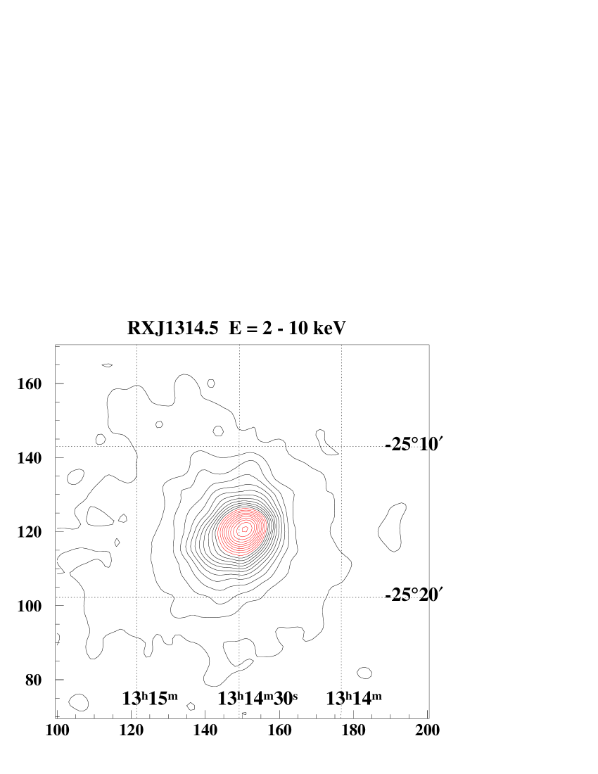
Figure 1: ASCA GIS images of our sample clusters: a RX J1023.8 in the 0.7 – 2 keV band, b RX J1023.8 in the 2 – 10 keV band, c RX J1031.6 in the 0.7 – 2 keV band, d RX J1031.6 in the 2 – 10 keV band, e RX J1050.5 in the 0.7 – 2 keV band, f RX J1050.5 in the 2 – 10 keV band, g RX J1203.2 in the 0.7 – 2 keV band, h RX J1203.2 in the 2 – 10 keV band, i RX J1314.5 in the 0.7 – 2 keV band, j RX J1314.5 in the 2 – 10 keV band. The pixel size is $0.25^{\prime}$ and the images have been filtered by a Gaussian having a $\sigma$ of 2 pixels. Contour levels are 1.0, 2.0, 3.0… counts/pixel.

Fig.2(a)

Fig.2(b)

Fig.2(c)

Fig.2(d)

Figure 2: ASCA spectra of individual clusters with the best-fitting MEKAL model: a RX J1023.8, b RX J1050.5, c RX J1203.2, d RX J1314.5. The upper panel shows the SIS0, SIS1, GIS2 and GIS3 spectra together with the best-fitting model. The lower panel shows the residual between the data and the best-fit model.

Figure 3: ASCA spectrum of RX J1031.6 with the best-fitting power-law model.

Figure 4: Temperature-luminosity relation. Triangles show our results including Paper I (Pierre et al. Pierre1999 (1999)) except for RX J1031.6-2607, and dots show nearby clusters ($z<0.1$) (Matsumoto et al. Matsumoto2000 (2000)).

Figure 5: Temperature-iron abundance relation. The symbols are the same as in Fig 4.

Figure 6: Redshift-iron abundance relation of our sample clusters.

Appendix A Contaminating source for RX J1050.5-0236

Fig. 7 shows the ASCA SIS (SIS0 + SIS1) image of RX J1050.5. The peak designated as “source 1” is RX J1050.5. Another peak (“source 2”) is conspicuous $\sim 6^{\prime}$ away from source 1. On the ROSAT HRI image, source 2 is pointlike and its position ( $(\alpha,\delta)_{\rm J2000}$ = (10h50m27.72s, -2d41m43.1s)) coincides with HD~93917, a K0 star (Lémonon Lemonon1999 (1999)). Despite the low number of photons in the ASCA image, we attempt to fit a single-thermal plasma model to this source: best-fit parameters are $N_{\rm H}=1.2\mbox{${}^{+1.1}_{-0.7}$}\mbox{$\times 10^{21}$}$ cm^-2, $kT=0.69\mbox{${}^{+0.16}_{-0.05}$}$ keV, $A_{\rm Fe}=0.14\mbox{${}^{+0.05}_{-0.04}$}$ solar, and $z=0.0(<0.057)$. The flux in the 0.5 – 10 keV band is 4.7$\times 10^{-13}$ erg s^-1 cm^-2. Spectra are displayed on Fig. 8.

Figure 7: ASCA SIS image of RX J1050.5-0236 in the 0.6 – 10.0 keV band. The pixel size is $6.3^{\prime\prime}$ and the image has been filtered by a Gaussian having a $\sigma$ of 1.5 pixel. Contours levels are 1.0, 2.0, 3.0…. counts/pixel. The regions extracted for the spectrum are indicated by circles.

Figure 8: ASCA spectra of source 2 in figure 7