Gravitational wave production: A strong constraint on primordial magnetic fields

Abstract

We compute the gravity waves induced by anisotropic stresses of stochastic primordial magnetic fields. The nucleosynthesis bound on gravity waves is then used to derive a limit on the magnetic field amplitude as function of the spectral index. The obtained limits are extraordinarily strong: If the primordial magnetic field is produced by a causal process, leading to a spectral index $n\geq 2$ on super horizon scales, galactic magnetic fields produced at the electroweak phase transition or earlier have to be weaker than $B_{\lambda}\leq 10^{-27}$Gauss! If they are induced during an inflationary phase (reheating temperature $T\sim 10^{15}$GeV) with a spectral index $n\sim 0$, the magnetic field has to be weaker than $B_{\lambda}\leq 10^{-39}$Gauss! Only very red magnetic field spectra, $n\sim-3$ are not strongly constrained. We also find that a considerable amount of the magnetic field energy is converted into gravity waves.

The gravity wave limit derived in this work rules out most of the proposed processes for primordial seeds for the large scale magnetic fields observed in galaxies and clusters.

]

I Introduction

Our galaxy, like most other spiral galaxies, is permeated by a magnetic field of the order of $B\sim 10^{-6}$Gauss. Recently, similar magnetic fields have also been observed in clusters of galaxies on scales of up to $\lambda\sim 0.1$Mpc [1, 2]. There is an ongoing debate whether such fields can be produced by charge separation processes during galaxy and cluster formation [3] or whether primordial seed fields are needed, which have then been amplified by simple adiabatic contraction or by a dynamo mechanism. In the first case, seed fields of $B\sim 10^{-9}$Gauss are needed while in the second case $B\sim 10^{-20}$Gauss [3] or even 10^-30Gauss in a universe with low mass density [4] suffice. Several mechanisms have been proposed for the origin of such seed fields, ranging from inflationary production of magnetic fields [5, 6, 7] to cosmological phase transitions [8].

Primordial magnetic fields have been constrained in the past in various ways mainly by using their effect on anisotropies in the cosmic microwave background [9, 10, 11, 12, 13, 14]. In these works constant magnetic fields and stochastic fields with red spectra $n\sim-3$ [14] have been considered and the limits obtained where of the order of a few$\times 10^{-9}$Gauss. A simple order of magnitude estimate shows that, from the CMB alone, one cannot expect much stronger constraints of magnetic fields: The energy density in a magnetic field is

$$\Omega_{B}={B^{2}\over 8\pi\rho_{c}}\simeq 10^{-5}\Omega_{\gamma}(B/10^{-8}{\rm Gauss})^{2}~{},$$ (1)

where $\Omega_{\gamma}$ is the density parameter in photons. We naively expect a magnetic field of $10^{-8}$Gauss to induce perturbations in the CMB on the order of $10^{-5}$, which are just on the level of the observed CMB anisotropies. It is thus expected that CMB anisotropies cannot constrain primordial magnetic fields to better than a few tenths of this amplitude.

In this work we constrain magnetic fields by the gravity waves which they induce classically, via the anisotropic stresses in their energy momentum tensor. These gravity waves lead to much stronger constraints than CMB anisotropies, especially for spectral indices $n>-3$. This comes from the fact that the spectrum of the gravity wave energy density induced by stochastic magnetic fields is always blue (except for $n=-3$ where it is scale invariant) and thus leads to stronger constraints on small scales than on the large scales probed by CMB anisotropies.

The effects of a constant magnetic field on gravity wave evolution and production have been studied in [16]. Here we concentrate on the production of gravity waves, but consider a stochastic magnetic field.

The remainder of this paper is organized as follows: In the next section we define the initial magnetic field spectrum and its evolution in time, and we determine the magnetic stress tensor which sources gravity waves. In Section 3 we calculate the induced gravity wave spectrum and estimate the effect of back-reaction. In Section 4 we derive limits on the primordial magnetic field using the nucleosynthesis limit on gravity waves and discuss our conclusions. In order not to loose the flow of the arguments, several technical derivations are deferred to three appendices.

We use conformal time which we denote by $\eta$; the scale factor is $a(\eta)$. Derivatives w.r.t conformal time are denoted by an over-dot, ${da\over d\eta}=\dot{a}$. We normalize the scale factor today to $a(\eta_{0})=1$. The index $0$ on a time dependent variable always indicates today. We assume a spatially flat universe with vanishing cosmological constant throughout. Neglecting a possible cosmological constant modifies the evolution of the scale factor only at very late times, $z<2$ and is therefore irrelevant for the results of this paper. We set the speed of light $c=1$ so that times and length scales can be given in units of sec, cm or Mpc, whatever is convenient. With our conventions, the scale factor is given by

$$a(\eta)=H_{0}\eta({H_{0}\eta\over 4}+\sqrt{\Omega_{\rm rad}})~{},$$ (2)

where $H_{0}=(3.086\times 10^{17}{\rm sec})^{-1}h_{0}$ is the Hubble parameter, $0.5<h_{0}<0.8$ and $\Omega_{\rm rad}=4.2\times 10^{-5}h_{0}^{-2}$ is the radiation density parameter (photons and three types of massless neutrinos).

Note that the scale factor has no units, but conformal time and comoving distance do. The normalization of $a$ implies that comoving distance becomes physical distance today. The conformal time $\eta$ is the comoving size of the horizon. The relation between $\eta$ and redshift or temperature is simply

$$z(\eta) = {1\over a(\eta)}-1~{},$$ (3)

$$T(\eta) = z(\eta)T_{0}\simeq z(\eta)2.4\times 10^{-4}{\rm eV}~{}.$$ (4)

The comoving time of equal matter and radiation, defined by $a(\eta_{eq})^{-3}=\Omega_{\rm rad}a(\eta_{eq})^{-4}$ or $z_{eq}+1=\Omega_{\rm rad}^{-1}$, is

$$\eta_{eq}=2(\sqrt{2}-1)\sqrt{\Omega_{\rm rad}}H_{0}^{-1}\sim 1.7\times 10^{15}{\rm sec}.$$ (5)

Greek indices run from $0$ to $3$, Latin ones from $1$ to $3$. Spatial (3d) vectors are denoted in bold.

II Primordial stochastic magnetic fields

In this section we closely follow Ref. [14]. During the evolution of the universe, the conductivity of the inter-galactic medium is effectively infinite. We can decouple the time evolution of the magnetic field from its spatial structure: B scales like $B^{2}(\eta,{\bf x})={\bf B}_{0}^{2}({\bf x})/a^{4}$ on sufficiently large scales. (In our coordinate basis $B_{i}\propto 1/a$ and $B^{i}\propto a^{-3}$ as can be derived easily from Maxwell’s equations in curved spacetime with vanishing electric field, see e.g. [17]). On smaller scales, the interaction of the magnetic field with the cosmic plasma becomes important, leading mainly to two effects: on intermediate scales, the field oscillates like $\cos(v_{A}k\eta)$, where $v_{A}=(B^{2}/(4\pi(\rho+p)))^{1/2}$ is the Alfvén velocity, and on very small scales, the field is exponentially damped due to shear viscosity [18, 19, 20]. We will take into account the time dependent damping scale as a time dependent cutoff $k_{d}(\eta)$ in the spectrum of ${\bf B}$. As we shall see, our constraints come from small scales where the spectrum is exponentially damped and oscillations can be ignored. We therefore disregard them in what follows. The expressions for $k_{d}(\eta)$ are derived in Appendix A. The only result of this appendix relevant here is that the damping scale $1/k_{d}(\eta)$ grows like a positive power $\alpha>0$ of $\eta$ and is always smaller than the horizon scale, $k_{d}(\eta)\propto 1/\eta^{\alpha}$ and $k_{d}(\eta)>1/\eta$. The reader not interested in the details of damping and confident with this relatively obvious result, can skip Appendix A.

We model ${\bf B}_{0}({\bf x})$ as a statistically homogeneous and isotropic random field. The transversal nature of ${\bf B}$ then leads to

$$\langle B^{i}({\bf k})B^{*j}({\bf q})\rangle=\delta^{3}({\bf k-q})(\delta^{ij}-\hat{k}^{i}\hat{k}^{j})B^{2}(k)~{}.$$ (6)

We use the Fourier transform conventions

$$\ B^{j}({\bf k}) = \int d^{3}x\exp(i{\bf x\cdot k})B_{0}^{j}({\bf x})~{},$$

$$B_{0}^{j}({\bf x}) = {1\over(2\pi)^{3}}\int d^{3}k\exp(-i{\bf x\cdot k})B^{j}({\bf k})~{},$$

and $\hat{\bf k}={\bf k}/k$, $k=\sqrt{\sum_{i}(k^{i})^{2}}$; ${\bf k}$ is the wave vector today which is also the co-moving wave vector. Its unit is inverse length which we will express in sec^-1.

We want to derive a limit on the amplitude of magnetic fields on the scale $\lambda\sim 0.1$Mpc generated by a primordial process which took place before $\eta=0.1{\rm Mpc}\sim 10^{13}{\rm sec}$ corresponding to $T\sim 1$keV. Hence we are mainly interested in magnetic fields generated on super horizon scales. As we shall see, our limits only apply for fields generated before nucleosynthesis, $T>T_{nuc}\simeq 0.1$MeV. The main examples we have in mind are inflationary generation of magnetic fields [5, 6], magnetic fields generated in string cosmology [7] and magnetic fields generated during the electroweak phase transition [8].

In the first two examples, a simple power law magnetic field spectrum with upper cutoff $k_{c}\simeq\eta_{in}^{-1}$ is generated. The conformal time $\eta_{in}$ marks the end of inflation or the string scale respectively.

Electroweak magnetic field production is causal, leading mainly to fields on scales smaller than the size of the horizon at the phase transition, $\eta_{ew}\simeq 4\times 10^{4}$sec $\simeq 10^{15}$cm $\simeq 3\times 10^{-4}$pc. These sub-horizon fields, which cannot propagate into larger scales during the linear evolution discussed in this paper, and which are essentially damped by viscosity, will be neglected in this paper. Motivated from inflation, we simply impose an initial cutoff scale $k_{c}(\eta_{in})=1/\eta_{in}$. Allowing for more small scale power, as it is certainly present initially in causal mechanisms, only strengthens our result which actually comes from the smallest scales not affected by damping.

If $\bf B$ is generated by a causal mechanism, it is uncorrelated on super horizon scales,

$$\langle B^{i}({\bf x},\eta)B^{j}({\bf x}^{\prime},\eta)\rangle=0~{}~{}~{}{\rm for}~{}~{}~{}|{\bf x}-{\bf x}^{\prime}|>2\eta~{}.$$ (7)

Here it is important, that the universe is in a stage of standard Friedman expansion, so that the comoving causal horizon size is about $\eta$. During an inflationary phase, the causal horizon diverges and our subsequent argument does not apply. In this somewhat misleading sense, one calls inflationary perturbations ’a-causal’.

According to Eq. (7), $\langle B^{i}({\bf x},\eta)B^{j}({\bf x}^{\prime},\eta)\rangle$ is a function with compact support and hence its Fourier transform is analytic. The function

$$\langle B^{i}({\bf k})B^{*j}({\bf k})\rangle\equiv(\delta^{ij}-\hat{k}^{i}\hat{k}^{j})B^{2}(k)$$ (8)

is analytic in k. If we assume also that $B^{2}(k)$ can be approximated by a simple power law, we must conclude that $B^{2}(k)\propto k^{n}$, where $n\geq 2$ is a even integer. (A white noise spectrum, $n=0$ does not work because of the transversality condition which has led to the non-analytic pre-factor $\delta^{ij}-\hat{k}^{i}\hat{k}^{j}$.) By causality, there can be no deviations from this law on scales larger than the horizon size at formation, $\eta_{in}$. As explained above, we neglect fields on smaller scales by a simple cutoff.

We assume that ${\bf B}_{0}$ is a Gaussian random field. Although this is not the most general case, it greatly simplifies calculations and gives us a good idea of what to expect in more general situations.

Using Wick’s theorem for Gaussian fields we can calculate the correlator of the tensor contribution to the anisotropic stresses induced by the magnetic field, which we denote by $\Pi_{ij}$. One finds (see Appendix B)

$$\langle\Pi^{ij}({\bf k},\eta)\Pi^{*lm}({\bf k}^{\prime},\eta)\rangle = |\Pi(k,\eta)|^{2}/a^{12}{\cal M}^{ijlm}\delta({\bf k-k^{\prime}})$$ (9)

$$\langle\Pi_{ij}({\bf k},\eta)\Pi^{*ij}({\bf k^{\prime}},\eta)\rangle = {4\over a^{8}}f^{2}(k,\eta)\delta({\bf k-k^{\prime}}),$$ (10)

where

$${\cal M}^{ijlm}({\bf k}) \equiv \delta^{il}\delta^{jm}+\delta^{im}\delta^{jl}-\delta^{ij}\delta^{lm}+k^{-2}(\delta^{ij}k^{l}k^{m}+$$ (13)

$$\delta^{lm}k^{i}k^{j}-\delta^{il}k^{j}k^{m}-\delta^{im}k^{l}k^{j}-\delta^{jl}k^{i}k^{m}$$

$$-\delta^{jm}k^{l}k^{i})+k^{-4}k^{i}k^{j}k^{l}k^{m}~{},$$

and

$$f(k)^{2}={1\over 16(2\pi)^{8}}\int d^{3}qB^{2}(q)B^{2}(|{\bf k}-{\bf q}|)(1+2\gamma^{2}+\gamma^{2}\beta^{2})~{},$$ (14)

with $\gamma={\bf\hat{k}}\cdot{\bf\hat{q}}$ and $\beta={\bf\hat{k}}\cdot{\widehat{\bf k-q}}$. For this result we made use of statistical isotropy, which implies that the two spin degrees of freedom of $\Pi_{ij}$ have the same average amplitude. More explicitly: in a coordinate system where ${\bf k}$ is parallel to the $z$-axis, $\Pi_{ij}$ has the form

$\displaystyle\left(\Pi_{ij}\right)=\left(\begin{array}[]{ccc}\Pi_{+}&\Pi_{\times}&0\\ \Pi_{\times}&-\Pi_{+}&0\\ 0&0&0\end{array}\right)~{};$

together with Eq. (10), statistical isotropy then gives

$$\langle|\Pi_{+}|^{2}\rangle=\langle|\Pi_{\times}|^{2}\rangle={1\over a^{4}}f^{2}~{}.$$ (15)

To continue, we have to specify $B^{2}(k)$. For simplicity we assume a simple power law with cutoff $k_{c}$ which can depend on time. As all scales smaller than $1/k_{d}(\eta)$ are damped, clearly we have to require $k_{c}(\eta)\leq k_{d}(\eta)$. Motivated by inflationary magnetic field production we choose $k_{c}(\eta_{in})\sim 1/\eta_{in}$, the primordial magnetic field is coherent up to the horizon size at formation. For magnetic fields produced during the electroweak phase transition, the ’coherence scale’ is substantially smaller [21], $k_{c}(\eta_{in})\gg 1/\eta_{in}$ which would strengthen our limit as we shall see. Since it is unphysical to assume $k_{c}(\eta_{in})<1/\eta_{in}$, our assumption is conservative. We set

$\displaystyle k_{c}(\eta)=\min(1/\eta_{in},k_{d}(\eta))~{}.$

It is important to keep in mind, that this cutoff scale is always smaller than the horizon scale.

We now can parameterize $B^{2}$ by

$$B^{2}(k)=\left\{\begin{array}[]{ll}{(2\pi)^{5}\over 2}{(\lambda/\sqrt{2})^{n+3}\over\Gamma[\frac{n+3}{2}]}B_{\lambda}^{2}k^{n}&\mbox{ for }k<k_{c}\\ 0&\mbox{ otherwise.}\end{array}\right.$$ (16)

The normalization is such that

$$B_{\lambda}^{2}={1\over V}\int d^{3}r\langle B_{0}({\bf x})B_{0}({\bf x}+{\bf r})\rangle\exp(-{r^{2}\over 2\lambda^{2}})~{},$$ (17)

where $V=\int d^{3}r\exp(-r^{2}/2\lambda^{2})=\lambda^{3}(2\pi)^{3/2}$ is the normalization volume. (We have assumed that the cutoff scale is smaller than $\lambda$.) We will finally fix $\lambda=0.1h^{-1}$Mpc, the largest scale on which coherent magnetic fields have been observed; but the scaling of our results with $\lambda$ will remain obvious.

The energy density in the magnetic field at some arbitrary scale $\ell$ is $\propto B_{\ell}^{2}\propto B^{2}(k)k^{3}|_{k=1/\ell}\propto\ell^{-(n+3)}$. In order not to over-produce long range coherent fields, we must require $n\geq-3$. For $n=-3$ we obtain a scale invariant magnetic field energy spectrum.

Using Eqs. (16) and (14) we can calculate $f$. The integral cannot be computed analytically, but the following result is a good approximation for all wave numbers $k$ [14]

$$f^{2}(k,\eta) \simeq A\times\left\{\begin{array}[]{ll}k_{c}(\eta)^{2n+3}&\mbox{ for }n\geq-3/2\\ k^{2n+3}&\mbox{ for }n\leq-3/2~{}.\end{array}\right.$$ (20)

with (21)

$$A = {(2\pi)^{3}\over 16}\frac{(\lambda/\sqrt{2})^{2n+6}B_{\lambda}^{4}}{\Gamma^{2}[\frac{n+3}{2}]}$$ (22)

For $n>-3/2$, the gravity wave source $\Pi$ is white noise, independent of $k$. Only the amplitude, which is proportional to $(\lambda k_{c})^{2n}$, depends on the spectral index. This is due to the fact that the integral (14) is dominated by the contribution from the smallest scale $k_{c}^{-1}$. The induced gravity wave spectrum will therefore be a white noise spectrum for all $n>-3/2$.

III Gravity waves from magnetic fields

We now proceed to calculate the gravity waves induced by the magnetic field stress tensor. The metric element of the perturbed Friedman universe is given by

$\displaystyle ds^{2}=a^{2}(\eta)[d\eta^{2}-(\delta_{ij}+2h_{ij})dx^{i}dx^{j}]~{},$

where $h^{i}_{i}=0$ and $h^{j}_{i}k^{i}=0$ for tensor perturbations. The magnetic field sources the evolution of $h_{ij}$ through

$${\ddot{h}}_{ij}+2{\dot{a}\over a}\dot{h}_{ij}+k^{2}h_{ij}=8\pi G\Pi_{ij}~{}.$$ (23)

$\Pi_{ij}$ is a random variable, but its time evolution is deterministic, it evolves in time simply by redshifting and by the evolution of the cutoff. Each component is given by

$\displaystyle\Pi_{\bullet}(k,\eta)={1\over a^{2}}f(k,\eta)\tilde{\Pi}_{\bullet}(k)~{},$

where $\tilde{\Pi}_{\bullet}(k)$ is a time independent random variable with power spectrum $\langle|\tilde{\Pi}_{\bullet}(k)|^{2}\rangle=1$. Therefore, also each component of the induced gravity wave is given by

$\displaystyle h_{\bullet}(k,\eta)=h(k,\eta)\tilde{\Pi}_{\bullet}(k)~{},$

where $h(k,\eta)$ is a solution of

$$\ddot{h}+2{\dot{a}\over a}\dot{h}+k^{2}h={8\pi G\over a^{2}(\eta)}f(k,\eta)~{}.$$ (24)

The gravity wave power spectrum is then given by

$$\langle\dot{h}^{ij}({\bf k},\eta)\dot{h}^{*}_{ij}({\bf k}^{\prime},\eta)\rangle=4\dot{h}^{2}(k,\eta)\delta({\bf k}-{\bf k}^{\prime})~{}.$$ (25)

In real space ,the energy density in gravity waves is

$\displaystyle\rho_{G}={\langle\dot{h}_{ij}\dot{h}^{ij}\rangle\over 16\pi Ga^{2}}~{}.$

The factor $1/a^{2}$ comes from the fact that $\dot{h}$ denotes the derivative w.r.t. conformal time. Fourier transforming this relation, we obtain with Eq. (25)

$$\rho_{G}=\int_{0}^{k_{c}}{dk\over k}{d\rho_{G}(k)\over d\log(k)}~{},$$ (26)

with

$\displaystyle{d\rho_{G}(k)\over d\log(k)}={k^{3}\dot{h}^{2}\over a^{2}(2\pi)^{6}G}$

such that

$${d\Omega_{G}(k)\over d\log(k)}\equiv{d\rho_{G}(k)\over\rho_{c}\,d\log(k)}={k^{3}\dot{h}^{2}\over a^{2}\rho_{c}(2\pi)^{6}G}~{},$$ (27)

where $\rho_{c}=3H_{0}^{2}/(8\pi G)$ denotes the critical density today. In Appendix C we solve Eq. (24) for $n<-3/2$, when $f$ is time independent, and we show that for wave numbers which enter the horizon in the radiation dominated era, the density parameter in gravity waves produced by the magnetic field can be expressed as

$${d\Omega_{G}(k)\over d\log(k)}\simeq{12k^{3}f(k)^{2}\log^{2}(x_{in})\over\rho_{c}^{2}\Omega_{\rm rad}(2\pi)^{5}}~{},$$ (28)

$$\mbox{ for }~{}n\leq-3/2~{}.$$ (29)

Fourier transforming the expression for the magnetic field energy $\rho_{B}=\langle B^{2}({\bf x})\rangle/(8\pi)$, we obtain the magnetic field density parameter at time $\eta$,

$${d\Omega_{B}(k)\over d\log(k)} = {B_{\lambda}^{2}\over 8\pi\rho_{c}}{(k\lambda)^{n+3}\over 2^{(n+3)/2}\Gamma({n+3\over 2})}$$ (30)

$$\Omega_{B}(\eta)=\Omega_{B}(k_{c}(\eta)) = \int_{0}^{k_{c}(\eta)}{dk\over k}{d\Omega_{B}(k)\over d\log(k)}$$ (31)

$$= {B_{\lambda}^{2}\over 8\pi\rho_{c}}{(k_{c}\lambda)^{n+3}\over 2^{(n+5)/2}\Gamma({n+5\over 2})}~{}.$$ (32)

Note that $\Omega_{B}$ may well be considerable on small scales, since this is the magnetic field energy at very early times which can be damped and transformed, e.g. into radiation later. But of course, for our perturbative calculation to apply, we must require ${d\Omega_{B}(k)\over d\log(k)}<\Omega_{\rm rad}$ during the radiation dominated era. Using Eqs. (30,32) and the result (20) for $f$, we obtain from Eq. (28)

$${d\Omega_{G}(k)\over d\log(k)} \simeq {({d\Omega_{B}(k)\over d\log(k)})^{2}\over\Omega_{\rm rad}}24\log^{2}(x_{in})~{},$$ (34)

$$\mbox{ for }-3<n<-3/2$$

$$\Omega_{G} = \int_{0}^{1/\eta_{in}}{dk\over k}{d\Omega_{G}(k)\over d\log(k)}$$ (35)

$$\simeq {\Omega_{B}^{2}(\eta_{in})\over\Omega_{\rm rad}}12(n+3)~{},$$ (37)

$$\mbox{ for }-3<n<-3/2~{}.$$

In the integrated formula for $\Omega_{G}$ we have neglected the logarithmic dependence $\log^{2}(x_{in})$.

If $n>-3/2$ the result changes since $f$ now depends on time via the cutoff $k_{c}(\eta)=\min(1/\eta_{in},k_{d}(\eta))$. Clearly, $k_{d}(\eta_{in})>1/\eta_{in}$ by causality. We define the time $\eta_{visc}$ to be the moment when the damping scale becomes smaller than $\eta_{in}$, $k_{d}(\eta_{visc})=1/\eta_{in}$. From that time on, the function $f$ decays like a power law,

$\displaystyle f^{2}(k,\eta)\propto k_{d}^{2n+3}\propto f^{2}(k,\eta_{in})(\eta_{visc}/\eta)^{\alpha(2n+3)}~{},$

where $\alpha$ is a positive power describing the growth of the viscosity damping scale. Hence, the source term of Eq. (24) starts to decay faster than $1/a^{2}$, and additional gravity wave production after $\eta_{visc}$ is sub-dominant. We neglect it in our attempt to derive an upper limit for primordial magnetic fields. For $n>-3/2$, the gravity wave solution given in Appendix C, Eq. (C5) is then simply modified by $-\log(x_{in})\rightarrow\log(x_{visc}/x_{in})$, since the integral of the gravity wave source term only has to extend from $x_{in}$ to $x_{visc}$. Taking also into account that up to $\eta_{visc}$ the cutoff scale is $k_{c}(\eta)=1/\eta_{in}$, hence $f^{2}(k,\eta)\propto k_{c}^{2n+3}=1/\eta_{in}^{2n+3}$, we obtain

$${d\Omega_{G}(k)\over d\log(k)} \simeq {\left({d\Omega_{B}(k)\over d\log(k)}\right)^{2}(k\eta_{in})^{-3-2n}\over\Omega_{\rm rad}}24\log^{2}(x_{visc}/x_{in}),$$ (39)

$$\mbox{ for }n>-3/2$$

$$\Omega_{G} \simeq {\Omega_{B}^{2}(\eta_{in})\over\Omega_{\rm rad}}8(n+3)^{2}\log^{2}(\eta_{visc}/\eta_{in})~{},$$ (41)

$$\mbox{ for }n>-3/2~{}.$$

In Appendix A, we estimate for the two examples of inflation, $T_{in}\sim 10^{15}$GeV, $\eta_{in}\sim 8\times 10^{-9}$sec and the electroweak phase transition, $T_{ew}\sim 200$GeV, $\eta_{in}=\eta_{ew}\sim 4\times 10^{4}$sec,

$$\eta_{visc}/\eta_{in}\simeq 10^{9} \eta_{in}=8\times 10^{-9}{\rm sec},$$ for inflation

$$\eta_{visc}/\eta_{ew}\stackrel{{\scriptstyle>}}{{\sim}}3000 \eta_{ew}\sim 4\times 10^{4}{\rm sec}~{}.$$ for ew. trans.

Up to logarithms, the final formula for gravity wave production is nearly the same for all values of the spectral index (cf. Eqs. (41) and (37)).

In these formulas back-reaction, namely the decrease of magnetic field energy due to the emission of gravity waves, is not included. Therefore Eqs. (34,37) and (39,41) are reasonable approximations only if $\Omega_{G}\stackrel{{\scriptstyle<}}{{\sim}}\Omega_{B}$. In the opposite case, which is realized whenever

$$\Omega_{B}(\eta_{in}) \stackrel{{\scriptstyle>}}{{\sim}} \Omega_{BG}(n)$$ (42)

$$\equiv \left\{\begin{array}[]{cc}{\Omega_{\rm rad}\over 12(n+3)}&\mbox{for }n<-3/2\\ {\Omega_{\rm rad}\over 8(n+3)^{2}\log^{2}(\eta_{visc}/\eta_{in})}&\mbox{for }n>-3/2\end{array}\right.$$ (45)

$$= \left\{\begin{array}[]{cc}{3.3\times 10^{-6}h_{0}^{-2}\over(n+3)}&\mbox{for }n<-3/2\\ {5\times 10^{-6}h_{0}^{-2}\over(n+3)^{2}\log^{2}(\eta_{visc}/\eta_{in})}&\mbox{for }n>-3/2~{},\end{array}\right.$$ (48)

the magnetic field energy is fully converted into gravity waves. Note, however, that the value $\Omega_{BG}(n)$ is in general not very much smaller than $\Omega_{\rm rad}$, which is an intrinsic limit on $\Omega_{B}$ for our perturbative approach.

In Fig. 1 the values $\Omega_{G}$ and $\Omega_{B}(\eta_{in})$ as functions of the spectral index are shown for two different choices of the creation time for the primordial magnetic field: the electroweak transition, $\eta_{in}=\eta_{ew}\sim 4\times 10^{4}$sec and inflation with $\eta_{in}\sim 8\times 10^{-9}$sec, for a magnetic field amplitude $B_{\lambda}=10^{-20}$ Gauss. They are compared with the nucleosynthesis limit, which comes from the fact that an additional energy density may not change the expansion law during nucleosynthesis in a way which would spoil the agreement of the calculated Helium abundance with the observed value. The maximum allowed additional energy density is given by [22]

$$\Omega_{\lim}h_{0}^{2}=1.12\times 10^{-6}~{}.$$ (49)

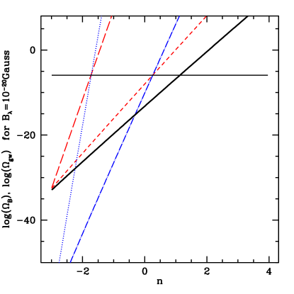
FIG. 1.: We show $\Omega_{G}h_{0}^{2}$ and $\Omega_{B}(\eta_{in})h_{0}^{2}$ as functions of the spectral index $n$ for two different times of primordial magnetic field creation: the electroweak transition ( $\Omega_{G}h_{0}^{2}$ dash-dotted, blue and $\Omega_{B}(\eta_{in})h_{0}^{2}$ short-dashed, red), and inflation ( $\Omega_{G}h^{2}$ dotted, blue and $\Omega_{B}(\eta_{in})h_{0}^{2}$ long-dashed, red) for a fiducial field strength $B_{\lambda}=10^{-20}$Gauss at $\lambda=0.1$Mpc. The nucleosynthesis limit, $\Omega_{\lim}h_{0}^{2}$ is also indicated. (The $\log$- terms have been neglected.) Clearly, the regimes with $\Omega_{B}>1$ or $\Omega_{G}>1$ are not physical and are just shown for illustration. We have also shown $\Omega_{B}(\eta_{nuc})h^{2}$, the magnetic field density which is simply cut off at the nucleosynthesis damping scale (fat solid line).

From Fig. 1 we see that $\Omega_{G}$ as calculated above dominates over $\Omega_{B}(\eta_{in})$ for all spectral indices $n>-2$ in the inflationary case and $n>0$ for electroweak magnetic field production, for an amplitude of $B_{\lambda}=10^{-20}$Gauss. This is due to the fact that we have neglected back-reaction which leads to a loss of magnetic field energy. Clearly, the magnetic field cannot convert more than all its energy into gravity waves. However, if our formula for $\Omega_{G}$ leads to $\Omega_{G}>\Omega_{B}(\eta_{in})$, it does actually convert most of its energy into gravity waves, before it is dissipated by plasma viscosity, since gravity wave production happens before and at horizon crossing, while viscosity damping is active only on scales which are well inside the horizon. We can take into account back-reaction by simply setting $\Omega_{G}\sim\Omega_{B}(\eta_{in})$ when our calculation gives $\Omega_{G}>\Omega_{B}(\eta_{in})$. We shall use this approximation for $\Omega_{G}$ in what follows.

Fig. 1 also shows that, since the value of the magnetic field density parameter at which conversion into gravity waves is quasi complete is so close to the nucleosynthesis limit, $\Omega_{BG}(n)h_{0}^{2}\sim 1.12\times 10^{-6}\equiv\Omega_{\lim}h_{0}^{2}$, the two curves $\Omega_{G}h_{0}^{2}$ and $\Omega_{B}(\eta_{in})h_{0}^{2}$ cross close to $\Omega_{\lim}h_{0}^{2}$. This means that the gravity wave limit for magnetic fields is very close to the limit obtained by setting $\Omega_{G}=\Omega_{B}(\eta_{in})$.

Let us discuss the problem of back-reaction in more detail. Even if $\Omega_{G}<\Omega_{B}(\eta_{in})$, as soon as ${d\Omega_{G}(k)\over d\log(k)}>{d\Omega_{B}(k)\over d\log(k)}$ for a given scale $k^{-1}$, we can no longer neglect back-reaction for this scale. The spectrum of $\Omega_{G}$ is

$\displaystyle{d\Omega_{G}(k)\over d\log(k)}\propto\left\{\begin{array}[]{cc}k^{2n+6},&\mbox{ for }n\leq-3/2\\ k^{3},&\mbox{ for }n\geq-3/2,\\ \end{array}\right.$

while ${d\Omega_{B}(k)\over d\log(k)}\propto k^{n+3}$. Hence for $-3<n<0$, the gravity wave spectrum is bluer than the magnetic field spectrum. Since there is no infrared cutoff, at sufficiently low values of $k$ we will always have ${d\Omega_{G}(k)\over d\log(k)}<{d\Omega_{B}(k)\over d\log(k)}$ and back reaction is unimportant at low $k$. The value $k_{\lim}$, below which this is the case, can be determined from Eqs. (30,34) and (39). We find

$$k_{\lim}\lambda\left(\log^{2}(k_{\lim}\eta_{in})\right)^{1\over n+3}\simeq\left({\Omega_{\rm rad}\over 24\Omega_{\lambda}}\right)^{1\over n+3}\sqrt{2}$$ (50)

$$\sim [10^{26}(10^{-20}{\rm Gauss}/B_{\lambda})^{2}]^{1\over n+3}\sqrt{2},$$ (52)

$$\mbox{ for }-3<n<-3/2$$

$$k_{\lim}\eta_{in}\simeq{1\over 2}\left({\sqrt{8}\Omega_{\rm rad}\over 24\Omega_{in}\log^{2}(\eta_{visc}/\eta_{in})}\right)^{-1\over n}$$ (53)

$$\sim \left[{2\times 10^{4}(10^{-9}{\rm Gauss}/B_{in})^{2}\over\log^{2}(\eta_{visc}/\eta_{in})}\right]^{-1\over n}~{},$$ (55)

$$\mbox{ for }-3/2<n<0,$$

where

$\displaystyle\Omega_{\lambda}=B^{2}_{\lambda}/(8\pi\rho_{c})\simeq\left({d\Omega_{B}(k)\over d\log(k)}\right)_{k=1/\lambda}~{}~{}\mbox{ and}$

$\displaystyle\Omega_{in}=\Omega_{\lambda}(\eta_{in}/\lambda)^{n+3}\simeq\left({d\Omega_{B}(k)\over d\log(k)}\right)_{k=1/\eta_{in}}~{},$

$B_{in}^{2}=B_{\lambda}^{2}(\lambda/\eta_{in})^{n+3}$.

If $k_{\lim}>1/\eta_{in}$, e.g. if the square bracket in Eq. (55) is larger than unity, back-reaction is never important.

For $n=0$ the magnetic field and gravity wave energy densities have the same spectral index and the condition that gravity wave back-reaction becomes important is scale independent. In this case it simply reads

$$\Omega_{in}\geq{\Omega_{\rm rad}\sqrt{8}\over 24\log^{2}(\eta_{visc}/\eta_{in})}~{}.$$ (56)

The situation is different for $n>0$. Then the gravity wave spectrum is less blue than the magnetic field spectrum and back reaction is always important at sufficiently low $k$, large scales.

When back reaction is important, it leads to damping of the primordial magnetic fields on large scales and will actually damp the field down to values for which back-reaction is unimportant. This can be seen as follows: gravity wave production takes place until $\Pi_{ij}(k)$, the tensor component of the magnetic field stress tensor, vanishes. But then $f^{2}(k)=0$ which implies according to Eq. (14)

$\displaystyle B^{2}(q)B^{2}(|{\bf k}-{\bf q}|)=0~{}~{}~{}\mbox{ for all}~{}~{}0\leq q\leq k_{c}.$

For $n<0$ the quadratic nature of the coupling of $B$ to gravity waves actually damps the magnetic field energy at least on all wave numbers $q>k_{\lim}/2$.

For $n>0$, back-reaction reduces $\Pi_{ij}(k)\propto\int d^{3}qB^{2}(q)B^{2}(|{\bf k}-{\bf q}|)$ for small enough values of $k$. In the limit $k\rightarrow 0$, this indicates that back-reaction damps the magnetic field on all scales until it becomes unimportant. It is difficult to decide without a detailed calculation how the magnetic field spectrum will actually be affected, but it seems reasonable to assume that back-reaction will alter it until $n\simeq 0$ and the amplitude until inequality (56) is violated. We can therefore assume that in late time magnetic fields inequality (56) is always violated if the magnetic field spectral index is $n\stackrel{{\scriptstyle>}}{{\sim}}0$.

We find this a very important result, which can be summarized as follows: Magnetic fields on super-horizon scale with a density which is sufficiently close to the radiation density are strongly damped into gravity waves when they enter the horizon. Note also that ’sufficiently close’ can even mean several orders of magnitude smaller since $\log^{2}(k\eta_{in})$ can easily become of order 100 or more. Furthermore, primordial magnetic fields produced on super horizon scales have their spectral index changed by gravity wave production to $n\stackrel{{\scriptstyle<}}{{\sim}}0$ once they enter the horizon.

During the matter dominated era gravity wave production is somewhat less efficient [14]; and since the scales of interest for us are sub-horizon in the matter era we do not discuss it here.

IV Limits and conclusions

The first limit for primordial magnetic fields produced before nucleosynthesis is simply that the energy density which they contribute may not change the expansion law during nucleosynthesis. As already mentioned, this condition implies [22]

$\displaystyle\Omega_{B}(\eta_{nuc})h_{0}^{2}\leq 1.12\times 10^{-6}=\Omega_{\lim}h_{0}^{2}~{}.$

Here we have disregarded the loss of magnetic field energy into gravity waves which will, as we shall see, strengthen the limit considerably. From Eq. (32) we have

$$\Omega_{B}(\eta_{nuc})={B_{\lambda}^{2}\over 8\pi\rho_{c}}{(k_{c}(\eta_{nuc})\lambda)^{n+3}\over 2^{n+5\over 2}\Gamma({n+5\over 2})}$$ (57)

$$~{}~{}~{}\simeq{4.5h_{0}^{-2}\!\times\!10^{-13}(5.9\!\times\!10^{6})^{n}\over 2^{n+5\over 2}\Gamma({n+5\over 2})}\!\left({B_{\lambda}\over 10^{-20}{\rm G}}\right)^{2}\!\left({\lambda\over 10^{13}{\rm sec}}\right)^{n+3}$$ (58)

where we have inserted
$k_{d}(\eta_{nuc})$ $\simeq$ $\sqrt{2\sigma_{T}\Omega_{b}\rho_{c}/(\eta_{nuc}^{3}m_{p}\Omega_{\rm rad}H_{0}^{2})}$ $\simeq$ $10^{5}/\eta_{nuc}$ $\simeq$ $6\times 10^{-7}$sec^-1 (for details see Appendix A and Refs. [19, 14, 20]). The density parameter $\Omega_{B}(\eta_{nuc})$ as a function of the spectral index $n$ is shown in Fig. 1.

Together with the above constraint, this gives already an interesting limit on primordial magnetic fields with spectral indices $n>-2$, as shown in Fig. 2 (solid line). For causal mechanisms of seed field production, $n\geq 2$, it even implies $B_{\lambda}<10^{-22}$Gauss.

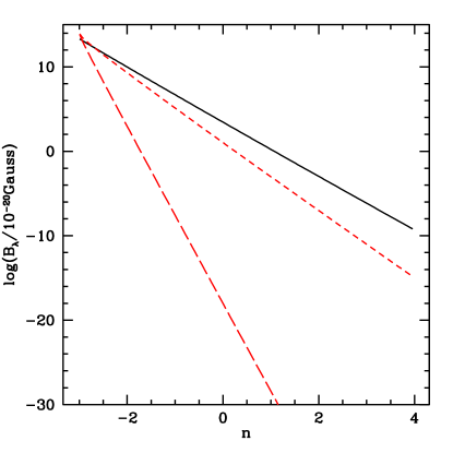
FIG. 2.: We show the nucleosynthesis limit on $B_{\lambda}$ (solid line) as function of the spectral index, $n$ together with the limit from gravity waves if the primordial field is produced at the electroweak transition (short-dashed) or during inflation (long-dashed) for $\lambda=0.1$h^-1Mpc$\simeq 10^{13}$sec.

Nevertheless, the limit implied from the production of gravity waves is more stringent, since the gravity waves have been produced at very early times, when the magnetic field damping scale was much smaller than $1/k_{d}(\eta_{nuc})\sim 1.7\times 10^{6}$sec. The production of gravity waves has prevented the magnetic field energy from being lost by viscosity damping, since gravity waves do not interact with matter in any substantial way.

Setting $\Omega_{G}=\Omega_{B}(\eta_{in})$ whenever the result of Eqs. (37,41) is larger than this limit, which is the simplest way to account for back-reaction, the condition

$$\Omega_{G}h_{0}^{2}<1.12\times 10^{-6}=\Omega_{\lim}h_{0}^{2}$$ (59)

yields the constraint for primordial magnetic fields created at $\eta_{in}$. For spectral indices

$\displaystyle n>-3+\sqrt{\Omega_{\rm rad}\over 8\Omega_{\lim}}\sim-1~{},$

the value for $\Omega_{G}$ inferred from Eq. (41) becomes larger than $\Omega_{B}(\eta_{in})$ at the limiting value $\Omega_{\lim}$ imposed from nucleosynthesis (in this approximation we have neglected the factor $\log^{2}(\eta_{visc}/\eta_{in})$, which can be considerable!). Then the magnetic field damping due to gravity wave productions is very important. But also for smaller values of the spectral index, $n>-3$, we have $\Omega_{G}\sim\Omega_{B}(\eta_{in})$ for $\Omega_{G}\sim\Omega_{\lim}$ and there is still a considerable amount of magnetic field damping due to gravity wave production.

The results for primordial magnetic fields produced at inflation and at the electroweak scale are shown in Fig. 2 (dashed lines). As can be seen for the two examples, primordial magnetic fields produced before nucleosynthesis are very strongly constrained. For all values of the spectral index, the following expression is a good approximation for the limit obtained:

$$B_{\lambda}/10^{-9}{\rm Gauss} < 700h_{0}\times(\eta_{in}/\lambda)^{(n+3)/2}{\cal N}(n)$$ (60)

$$\mbox{where }~{}{\cal N}(n) \equiv \sqrt{2^{n+5\over 2}\Gamma\left({n+5\over 2}\right)}\sim 1~{}.$$ (61)

This nucleosynthesis bound becomes stronger for smaller cutoff scales, larger $k_{c}$, according to Eq. (60) it scales like $(k_{c}\lambda)^{-(n+3)/2}$. (Remember that we have set $k_{c}=1/\eta_{in}$.)

If the seed field is produced during an inflationary phase at GUT scale temperatures, where conformal invariance can be broken e.g. by the presence of a dilaton, the induced fields must be smaller than $B_{\lambda}\sim 10^{-20}$Gauss for $n>-2$. If seed fields are produced after inflation, their spectrum is constrained by causality. Deviation from a power law with $n\geq 2$ can only be produced on sub-horizon scales, $k>1/\eta_{in}$. Therefore our limit derived by setting $B(k)=0$ on sub-horizon scales, $k\eta_{in}>1$, is the most conservative choice consistent with causality.

Mechanisms which still can produce significant seed fields are either ’ordinary’ inflation, if the spectral index $n\stackrel{{\scriptstyle<}}{{\sim}}-2$ or a late inflationary phase at the electroweak scale (or even later) where a seed field with $n\stackrel{{\scriptstyle<}}{{\sim}}0$ can have amplitudes of $B_{\lambda}\sim 10^{-20}$Gauss.

We also have found that magnetic fields which contribute an energy density close to the nucleosynthesis bound, loose a considerable amount (if not all) of their energy into gravity waves, which might be detectable. In fact, the space born interferometer approved by the European Space Agency and NASA, the Large Interferometer Space Antenna (LISA) which has its most sensitive regime where it can detect $\Omega_{G}h_{0}^{2}\sim 10^{-11}$ around $10^{-3}$Hz$\sim 1/\eta_{weak}$ [22] will either detect or rule out all magnetic seed fields with spectral index $n\stackrel{{\scriptstyle>}}{{\sim}}-0.5$ produced around or before the electroweak phase transition. If LISA does not detect a gravity wave background, the constraint analogous to Eq. (60) for $\eta_{in}\leq 4\times 10^{4}$sec yields

$\displaystyle B_{\lambda}<10^{-20}{\rm Gauss}~{}~{}\mbox{ for all indices }n>-0.5$

for all mechanisms producing seed fields before or at the electroweak phase transition.

We conclude that, most probably, magnetic seed fields have to be produced relatively late, or after nucleosynthesis to evade the discussed bounds. Our gravity wave bound is not relevant for magnetic fields which are produced on sub-horizon scales. But for $\lambda\stackrel{{\scriptstyle>}}{{\sim}}0.1$Mpc to enter the horizon, this requires a temperature of creation $T<1$keV. The only late time mechanism found so far which could lead to seed fields is recombination, where large scale fields of the order of $B\sim 10^{-20}$ Gauss can be induced by magneto-hydrodynamic effects, and the difference in the viscosity of electrons and ions [23], a charge separation mechanism. Our work strongly constrains processes of quantum particle production (during e.g. an inflationary phase) as origin for the observed magnetic fields and favors more conventional processes like charge separation in the late universe.

Acknowledgment:    We thank Pedro Ferreira, Michele Maggiore and Roy Maartens for helpful discussions. This work is supported by the Swiss NSF.

A Damping of magnetic fields by viscosity

In this appendix we determine the cutoff function $k_{d}(\eta)$. We use the results found in [19, 18] and [20].

We split the magnetic field into a high frequency and a low frequency component, separated by the Alfvén scale, $\lambda_{A}=v_{A}\eta$, where the Alfvén velocity

$\displaystyle v_{A}^{2}={\langle B^{2}\rangle\over 4\pi(\rho_{r}+p_{r})}$

depends on the low frequency component: $\langle B^{2}_{A}\rangle=\langle B_{0i}({\bf x})B_{0}^{i}({\bf x})\rangle|_{\lambda_{A}}$, $v_{A}\sim 4\times 10^{-4}\times(B_{A}/10^{-9}{\rm Gauss})$  [14]. The amplitude of the high frequency component then obeys a damped harmonic oscillator equation, with damping coefficient, $D(\eta)$, depending on time and on the mean free path of the diffusing particles giving rise to viscosity [19]. In the oscillatory regime, we define the damping scale at each time $\eta$ to be the scale at which one e-fold of damping has occurred: $\int_{0}^{\eta}\frac{D}{2}d\eta=1$. The damping term $D$ is given by $D=k^{2}\lambda_{col}/a(\eta)$, where $\lambda_{col}$ is the mean free path of the particle species with the highest viscosity which is still sufficiently strongly coupled to the magnetic field. Long wave modes with $1/k>v_{A}\eta$ are not significantly damped. We now determine the damping scale as a function of time. To determine whether a given mode with $k>k_{d}(\eta)$ is effectively damped one has to decide whether it is in the oscillatory regime, $\omega_{0}=kv_{A}>D=k^{2}\lambda_{col}/a(\eta)$ where damping really has time to occur or in the ’over-damped’ regime $k<v_{A}a(\eta)/2\lambda_{col}$ where amplitudes remain approximatively constant. With $v_{A}$ this depends on the magnetic field under consideration.

Let us now determine the damping scale. Before neutrino decoupling at $T\stackrel{{\scriptstyle>}}{{\sim}}1$MeV corresponding to $\eta\stackrel{{\scriptstyle<}}{{\sim}}10^{10}$sec, damping is due to both photon and neutrino viscosity. The mean free path of photons is

$$\lambda_{col,\gamma}\simeq\frac{1}{\sigma_{T}n_{e}}\simeq a^{3}(1.5\times 10^{20}\mathrm{sec})~{},$$

where $\sigma_{T}=6.65\times 10^{-25}{\rm cm}^{2}$ is the cross section of Thomson scattering. For neutrinos, we take into account scattering with leptons as the principle scattering process giving rise to viscosity:

$$\lambda_{col,\nu}\simeq\frac{1}{\sigma_{w}n_{\nu}}\simeq a^{5}(7\times 10^{48}\mathrm{sec})~{},$$

where $\sigma_{w}=G_{F}^{2}T^{2}$ is the weak cross section and $G_{F}=(293{\rm GeV})^{-2}$ is Fermi’s constant. Note that we set $\hbar=c=1$ so that a cross section also can have the units GeV^-2.

Using the expression for the scale factor given in Eq. (2), one finds that photon viscosity dominates until $\eta\simeq 10^{5}$ sec, leading to

$$k_{d}(\eta)\simeq(2\times 10^{10}\mathrm{sec}^{1/2})\eta^{-3/2}~{}.$$ (A1)

For $\eta>10^{5}$ sec neutrinos viscosity takes over, with cutoff function

$$k_{d}(\eta)=(4\times 10^{15}\mathrm{sec}^{3/2})\eta^{-5/2}$$ (A2)

during the oscillatory regime. The comoving wavenumber $k$ is given here in units of sec^-1.

After $\eta\stackrel{{\scriptstyle>}}{{\sim}}10^{10}$sec neutrinos decouple and the dominant viscosity is again photon viscosity leading to the cutoff function (A1).

Estimating the viscosity time, namely $k_{d}(\eta_{visc})=1/\eta_{in}$ for inflation, $\eta_{in}\sim 10^{-8}$sec and the electroweak phase transition, $\eta_{in}=\eta_{ew}\simeq 4\times 10^{4}$sec, we find from the expressions above $\eta_{visc}/\eta_{in}|_{\rm inflation}\sim 3\times 10^{9}$ and $\eta_{visc}/\eta_{ew}\sim 3000.$ The first result is calculated using photon viscosity is just approximative, since we do not know the relevant cross sections up to the scale of inflation, $10^{15}$GeV, but we certainly expect the value to be very large, since interactions are strong and thus viscosity is weak. The electroweak result, calculated using the neutrino viscosity, would be quite reliable in the oscillatory regime. However, for magnetic fields $B<10^{-9}$Gauss, for which the Alfvén velocity is smaller than $10^{-4}$, the scale $\eta_{visc}$ is still in the over-damped regime. The time at which the scale can then effectively be damped depends on the value of the magnetic field. In this sense our result is only a lower limit, $\eta_{visc}/\eta_{ew}\stackrel{{\scriptstyle>}}{{\sim}}3000.$ This is not very important for our final bounds, where we will even set $\log{\eta_{visc}/\eta_{in}}\sim 1$, in order to obtain results which are independent of the time of magnetic field creation.

As an example we also determine the damping scale at nucleosynthesis, $T\simeq 0.1$MeV, $z_{nuc}\simeq 4\times 10^{8}$ which we need in Section 4. Setting $D\eta/2=1$, we obtain

$$k_{d}(\eta_{nuc})=[2a(\eta_{nuc})\sigma_{T}n_{e}(\eta_{nuc})/\eta_{nuc}]^{1/2}~{}.$$ (A3)

Using $n_{e}=\rho_{c}\Omega_{b}/(m_{p}a^{3})$, where $m_{p}$ is the proton mass, as well as our expression for the scale factor one obtains

$\displaystyle k_{d}(\eta_{nuc})\simeq 6\times 10^{-7}{\rm sec}^{-1}\simeq 10^{5}/\eta_{nuc}$

This can of course also be obtained by simply using $\eta_{nuc}\simeq 10^{11}$sec in the above function for photon viscosity given in Eq. (A1). Again, whether or not this scale is in the oscillatory regime and can be effectively damped, depends on the value of $B(k_{d})$. For $B(k_{d})\sim 10^{-6}$Gauss, which satisfies the nucleosynthesis bound, this is largely the case, and for magnetic fields of interest to us $k_{d}(\eta_{nuc})$ is the correct damping scale.

At the end of the radiation dominated era, photons decouple and viscosity acts no more. Since gravity wave production in the matter dominated regime is not important, we do not calculate the cutoff function in this regime.

B The gravity wave source of stochastic magnetic fields

The Maxwell stress tensor of a magnetic field in real space is given by

$$T^{ij}({\bf x},\eta) = {1\over 4\pi}\big{[}B^{i}({\bf x},\eta)B^{j}({\bf x},\eta)$$

$$-{1\over 2}g^{ij}({\bf x},\eta)B_{n}({\bf x},\eta)B^{n}({\bf x},\eta)\big{]}~{}.$$

In Fourier space, using the Fourier transform convention adopted in this paper and the scaling of the magnetic field with time, we have

$$T^{ij}({\bf k},\eta) = {1\over 4\pi(2\pi)^{3}a^{6}}\int d^{3}q\big{[}B^{i}({\bf q})B^{j}({\bf k-q})$$ (B2)

$$-{1\over 2}B^{l}({\bf q})B^{l}({\bf k-q})\delta^{ij}\big{]}~{},$$

where we have introduced the factor $1/a^{6}$ to transform the present field $B^{i}({\bf k})=B^{i}({\bf k},\eta_{0})$ back to the physical field $B^{i}({\bf k},\eta)=B^{i}({\bf k})/a^{3}$. $\Pi^{ij}({\bf k},\eta)$ is the transverse traceless component of $T^{ij}({\bf k},\eta)$, which sources gravity waves. Here we give the details of the calculation of its correlation function, $\langle\Pi^{ij}({\bf k},\eta)\Pi^{*lm}({\bf k}^{\prime}\eta)\rangle$ which we use to compute the induced gravity waves. The projector onto the component of a vector transverse to ${\bf k}$ is $P_{ij}=\delta_{ij}-\hat{k}_{i}\hat{k}_{j}$. Consequently $P^{i}_{a}P^{j}_{b}$ projects onto the transverse component of a tensor. To obtain the transverse traceless component we still have to subtract the trace. Hence defining the projector

$\displaystyle{\mathcal{P}}^{ij}_{ab}=P^{i}_{a}P^{j}_{b}-{1\over 2}P^{ij}P_{ab}$

we have

$$\langle\Pi^{ij}({\bf k},\eta)\Pi^{*lm}({\bf k}^{\prime},\eta)\rangle={\mathcal{P}}^{ij}_{~{}~{}ab}{\mathcal{P}}^{lm}_{~{}~{}cd}\langle T^{ab}({\bf k},\eta)T^{*cd}({\bf k}^{\prime},\eta)\rangle\>.$$ (B3)

To simplify the calculation, we note that up to a trace, which anyway vanishes in the projection (B3), $T^{ab}({\bf k},\eta)$ is just given by

$$\Delta^{ab}({\bf k},\eta)\equiv{1\over 4\pi(2\pi)^{3}a^{6}}\int d^{3}qB^{a}({\bf q})B^{b}({\bf k-q})~{}.$$ (B4)

We therefore can write

$$\langle\Pi^{ij}({\bf k},\eta)\Pi^{*lm}({\bf k}^{\prime},\eta)\rangle={\mathcal{P}}^{ij}_{~{}~{}ab}{\mathcal{P}}^{lm}_{~{}~{}cd}\langle\Delta^{ab}({\bf k},\eta)\Delta^{*cd}({\bf k}^{\prime},\eta)\rangle\>.$$ (B5)

To compute the two point correlator of $\Delta$, we use expression (B4) and the assumption that the random magnetic field be Gaussian, so that we can apply Wick’s theorem. In other words, products of four magnetic fields can be reduced by

$$\langle B^{i}({\bf k})B^{*j}({\bf q})B^{n}({\bf s})B^{*m}({\bf p})\rangle=~{}~{}~{}~{}~{}~{}~{}~{}~{}~{}$$ (B9)

$$~{}~{}~{}~{}~{}~{}~{}~{}~{}~{}\langle B^{i}({\bf k})B^{*j}({\bf q})\rangle\langle B^{n}({\bf s})B^{*m}({\bf p})\rangle+$$

$$~{}~{}~{}~{}~{}~{}~{}~{}~{}~{}\langle B^{i}({\bf k})B^{n}({\bf s})\rangle\langle B^{*j}({\bf q})B^{*m}({\bf p})\rangle+$$

$$~{}~{}~{}~{}~{}~{}~{}~{}~{}~{}\langle B^{i}({\bf k})B^{*m}({\bf p})\rangle\langle B^{n}({\bf s})B^{*j}({\bf q})\rangle~{}.$$

Using also the reality condition, $B^{*a}({\bf k})=B^{a}(-{\bf k})$, and the two point correlator (6), we obtain

$$\langle\Delta^{ab}({\bf k},\eta)\Delta^{*cd}({\bf k}^{\prime},\eta)\rangle=\frac{a^{-12}}{4(2\pi)^{8}}\int d^{3}qd^{3}p[\delta({\bf k})\delta({\bf k}^{\prime})\times$$ (B10)

$$B^{2}(q)B^{2}(-p)(\delta^{ab}-\hat{q}^{a}\hat{q}^{b})(\delta^{cd}-\hat{p}^{c}\hat{p}^{d})+$$ (B11)

$$+\delta({\bf q}-{\bf p})\delta({\bf k}-{\bf q}-{\bf k}^{\prime}+{\bf p})B^{2}(q)B^{2}(|{\bf k}-{\bf q}|)\times$$ (B12)

$$~{}~{}~{}(\delta^{ac}-\hat{q}^{a}\hat{q}^{c})(\delta^{bd}-(\widehat{{\bf k}-{\bf q}})^{b}(\widehat{{\bf k}-{\bf q}})^{d})+$$ (B13)

$$+\delta({\bf q}-{\bf k}^{\prime}+{\bf p})\delta({\bf k}-{\bf q}-{\bf p})B^{2}(q)B^{2}(|{\bf k}-{\bf q}|)\times$$ (B14)

$$~{}~{}(\delta^{ad}-\hat{q}^{a}\hat{q}^{d})(\delta^{bc}-(\widehat{{\bf k}-{\bf q}})^{b}(\widehat{{\bf k}-{\bf q}})^{c})].$$ (B15)

The first term only contributes an uninteresting constant and can be disregarded. For the remaining two terms integration over $d^{3}p$ eliminates one of the two $\delta$-functions and leads to

$$\langle\Delta^{ab}({\bf k},\eta)\Delta^{*cd}({\bf k^{\prime}},\eta)\rangle=$$ (B19)

$$\delta({\bf k}-{\bf k^{\prime}}){a^{-12}\over 4(2\pi)^{8}}\int d^{3}q~{}B^{2}(q)B^{2}(|{\bf k}-{\bf q}|)\times$$

$$\left[(\delta^{ac}-{\hat{q}}^{a}{\hat{q}}^{c})(\delta^{bd}-{\widehat{({\bf k}-{\bf q})}}^{b}{\widehat{({\bf k}-{\bf q})}}^{d})+\right.$$

$$\left.(\delta^{ad}-{\hat{q}}^{a}{\hat{q}}^{d})(\delta^{bc}-{\widehat{({\bf k}-{\bf q})}}^{b}{\widehat{({\bf k}-{\bf q})}}^{c})\right]~{}.$$

Clearly, the correlator of $\Delta$ and thus also the one of $\Pi$ is symmetric in ${\bf k}$ and ${\bf k}^{\prime}$ and hence also under the exchange of the first and the second pair of indices. In addition it is symmetric in the first and the second as well as in the third and the fourth index. The most general isotropic transverse traceless fourth rank tensor which obeys these symmetries has the tensorial structure

$${\cal M}^{ijlm}({\bf k}) = \delta^{il}\delta^{jm}+\delta^{im}\delta^{jl}-\delta^{ij}\delta^{lm}+k^{-2}(\delta^{ij}k^{l}k^{m}+$$ (B22)

$$\delta^{lm}k^{i}k^{j}-\delta^{im}k^{j}k^{l}-\delta^{il}k^{j}k^{m}-\delta^{jl}k^{i}k^{m}$$

$$-\delta^{jm}k^{i}k^{l})+k^{-4}k^{i}k^{j}k^{l}k^{m}~{}.$$

We could not find a straight forward derivation of this result in a textbook on multi-linear algebra where it actually belongs, but it can be found, e.g. in [24].

We can hence set

$$\langle\Pi^{ij}({\bf k},\eta)\Pi^{*lm}({\bf k}^{\prime},\eta)\rangle = f(k,\eta)^{2}/a^{12}{\cal M}^{ijlm}\delta({\bf k-k^{\prime}})$$ (B23)

with (B24)

$$\langle\Pi_{ij}({\bf k},\eta)\Pi^{*ij}({\bf k^{\prime}},\eta)\rangle = {4\over a^{8}}f(k,\eta)^{2}\delta({\bf k-k^{\prime}}),$$ (B25)

To determine the correlator of $\Pi$ it is therefore sufficient to calculate its trace. With ${\mathcal{P}}_{ijab}{\mathcal{P}}^{ij}_{cd}={\mathcal{P}}_{abij}{\mathcal{P}}_{cd}^{ij}={\mathcal{P}}_{abcd}$, (for the last identity we simply use that projectors are idem-potent), we have

$$\langle\Pi_{ij}({\bf k},\eta)\Pi^{*ij}({\bf k^{\prime}},\eta)\rangle={\mathcal{P}}^{abcd}\langle\Delta_{ab}({\bf k},\eta)\Delta_{*cd}({\bf k^{\prime}},\eta)\rangle~{}.$$ (B26)

A somewhat tedious but straight forward computation gives

$${\mathcal{P}}^{abcd}[(\delta^{ac}-\hat{q}^{a}\hat{q}^{c})(\delta^{bd}-(\widehat{{\bf k}-{\bf q}})^{b}(\widehat{{\bf k}-{\bf q}})^{d})$$ (B27)

$$~{}~{}\qquad+(\delta^{ad}-\hat{q}^{a}\hat{q}^{d})(\delta^{bc}-(\widehat{{\bf k}-{\bf q}})^{b}(\widehat{{\bf k}-{\bf q}})^{c})]=$$ (B28)

$$1+(\hat{{\bf k}}\!\cdot\!(\widehat{{\bf k}\!-\!{\bf q}}))^{2}+(\hat{{\bf k}}\!\cdot\!\hat{{\bf q}})^{2}+(\hat{{\bf k}}\!\cdot\!\hat{{\bf q}})^{2}(\hat{{\bf k}}\!\cdot\!(\widehat{{\bf k}\!-\!{\bf q}}))^{2}\>.$$ (B29)

Setting $\gamma=\hat{{\bf k}}\cdot\hat{{\bf q}}$ and $\beta=\hat{{\bf k}}\cdot(\widehat{{\bf k}-{\bf q}})$, and using the fact that the second term transforms into the third one under the transformation ${\bf q}\rightarrow{\bf k}-{\bf q}$, we finally obtain

$$\langle\Pi_{ij}({\bf k},\eta)\Pi^{*ij}({\bf k}^{\prime},\eta)\rangle=\frac{a^{-8}}{4(2\pi)^{8}}\delta({\bf k}-{\bf k})\times$$ (B30)

$$\qquad\int d^{3}qB^{2}(q)B^{2}(|{\bf k}-{\bf q}|)(1+2\gamma^{2}+\gamma^{2}\beta^{2})\>,$$ (B31)

which leads to the result for $f(k)$ given in Eq. (14).

C Gravitational wave production

The equation for gravity wave production due to tensor type anisotropic stresses is

$${\ddot{h}}_{ij}+2{\dot{a}\over a}\dot{h}_{ij}+k^{2}h_{ij}=8\pi G\Pi_{ij}~{}.$$ (C1)

For each mode we therefore have an equation of the form

$${\ddot{h}}+2{\dot{a}\over a}\dot{h}+k^{2}h=s(k,\eta)~{},$$ (C2)

where $s(k,\eta)={8\pi G\over a^{2}}f(k,\eta)$. The function $f$ only depends on $\eta$ for $n>-3/2$ via the damping cutoff $k_{d}(\eta)$. In terms of the dimensionless variable $x=k\eta$ equation (C2) reduces to

$$h^{\prime\prime}+2{\alpha\over x}h^{\prime}+h=s(k,\eta)k^{-2}~{},$$ (C3)

where $\alpha=1$ in the radiation dominated era, and $\alpha=2$ in the matter dominated era. The homogeneous solutions of Eq. (C3) are the spherical Bessel functions $j_{0}~{},y_{0}$ in the radiation dominated era, and $j_{1}/x,~{}y_{1}/x$ in the matter dominated era respectively. We assume that the magnetic fields were created in the radiation dominated epoch, at redshift $z_{in}$. Using the Wronskian method, the general solution of Eq. (C3) which vanishes at $z_{in}$ is given by

$$h(x)=c_{1}(x)g_{1}(x)+c_{2}(x)g_{2}(x)~{},$$ (C4)

where $g_{1},g_{2}$ are the above mentioned homogeneous solutions and

$$c_{1}(x) = -k^{-2}\int_{x_{in}}^{x}s(x^{\prime})g_{2}(x^{\prime})/W(x^{\prime})dx^{\prime}$$

$$c_{2}(x) = k^{-2}\int_{x_{in}}^{x}s(x^{\prime})g_{1}(x^{\prime})/W(x^{\prime})dx^{\prime}~{},$$

$W=g_{1}g_{2}^{\prime}-g_{1}^{\prime}g_{2}$ is the Wronskian determinant of the homogeneous solution. Inside the horizon the homogeneous solutions $g_{1}$ and $g_{2}$ begin to oscillate. The contribution to the integral from times where the scale under consideration is sub-horizon is hence negligible. Furthermore, since the gravity wave energy is growing with wave number (it is proportional to $k^{3}f^{2}$), our limit will come from large wave numbers, small scales, which enter the horizon before decoupling. Let us thus solve Eq. (C3) explicitly in the radiation dominated regime, $\eta<\eta_{eq}$, for a wave number which enters the horizon in the radiation era, $k\eta_{eq}>1$, and in the case where $f$ is not time dependent ($n<-3/2$). We first notice that the Wronskian $W(j_{0},y_{0})=1/x^{2}$. Using the radiation approximation of  Eq. (2) for the scale factor, $a=H_{0}\eta\sqrt{\Omega_{\rm rad}}$ we have

$\displaystyle{k^{-2}s(x)\over W(x)}={8\pi Gf(k)\over H_{0}^{2}\Omega_{\rm rad}}~{}.$

Since $y_{0}$ diverges at small $x$ the term $c_{1}$ clearly dominates. After horizon crossing we have

$\displaystyle h(x)\simeq c_{1}(1)j_{0}(x)=c_{1}(1){\sin x\over x}~{}.$

Performing the integral $c_{1}(1)$, we find

$$h(x)\simeq-{8\pi Gf(k)\over H_{0}^{2}\Omega_{\rm rad}}{\sin x\over x}\log(x_{in})~{},$$ (C5)

for $x>1$ and $\eta<\eta_{eq}\simeq\sqrt{\Omega_{\rm rad}}/H_{0}$. We have compared this formula with the numerical solution and, as expected, found that it is a very reasonable approximation (within less than 10% of the numerical result).

After horizon crossing, the gravity waves thus propagate freely, and their energy just scales like radiation energy, so that for $k\eta_{eq}>1$, using Eq. (27)

$${d\Omega_{G}(k)\over d\log(k)} \simeq {d\rho_{G}(k)\over\rho_{\rm rad}\,d\log(k)}\Omega_{\rm rad}={k^{3}\dot{h}^{2}\over a^{2}\rho_{\rm rad}(2\pi)^{6}G}\Omega_{\rm rad}~{}.$$ (C6)

During the radiation era, on sub-horizon scales

$\displaystyle\dot{h}\simeq{8\pi Gf(k)\over\eta H_{0}^{2}\Omega_{\rm rad}}\log(x_{in})\cos(x)\mbox{ and }a^{2}\rho_{\rm rad}={3\over 8\pi G}\left({1\over\eta}\right)^{2}$

so that

$${d\Omega_{G}(k)\over d\log(k)} = {4k^{3}f(k)^{2}(8\pi G)^{2}\log^{2}(x_{in})\cos^{2}(x)\over H_{0}^{4}\Omega_{\rm rad}3(2\pi)^{5}}$$ (C7)

$$\simeq {12k^{3}f(k)^{2}\log^{2}(x_{in})\over\rho_{c}^{2}\Omega_{\rm rad}(2\pi)^{5}}~{}.$$ (C8)

Since the ratio between the gravity wave energy density and the radiation energy density is time independent, this formula is valid also in the matter era. $\rho_{c}=3H_{0}^{2}/(8\pi G)$ denotes the critical density today.