The velocity field of collapsing spherical structures

We assume that the amplitude of the caustics in redshift space is a sum of two components: the first one can be predicted by the spherical infall model with no random motion, and the second is due to the random motion distribution. Smooth model curves are used to estimate the maximum values of the first component for the Coma cluster. Then, an approximation of the radial component of the infall velocity –based on the above curves– is derived and a mass profile of the cluster is calculated. This mass profile, that is an upper limit for the spherical infall model, combined with estimations given by other authors provides an approximation of a lower limit for the mass of the system.

1 Introduction

The spherical infall model has been extensively discussed in the literature (Gunn & Gott gunn72 (1972); Silk silk (1974); Gunn gunn77 (1977); Peebles (peeb76 (1976), peeb80 (1980)); Schechter schechter (1980); Schectman shectman (1982); Ostriker et al. ostriker (1988)). This model assumes that galaxy clusters started as small density perturbations in the early universe. These perturbations eventually deviate from the general expansion and after reaching a maximum radius they start collapsing. The most probable scenario is that galaxies formed during the expansion phase of their cluster. Thus, the cluster consists of largely individual galaxies during its collapse.

The observed velocities of these galaxies (along the line–of–sight) give important information about the dynamical state of the cluster (Kaiser kaiser (1987)). Regös & Geller (regos (1989)) showed that plotting the observed velocities of galaxies as function of their angular distances from the centre of the cluster one obtains a velocity distribution that is bounded by sharp, characteristic trumpet–shaped curves. These curves, called caustics, form an envelope containing the galaxies of the cluster. The caustics are used to estimate the density parameter $\Omega_{0}$ of the universe (Regös & Geller regos (1989)) and the mass profile for the galaxy clusters (Geller et al. gell99 (1999); Reisenegger et al. reinse (2000)). In Sect. 2, we show that the form of the caustics fully defines the profile of the radial infall velocity in the case of a pure spherical collapse. In Sect. 3, we describe the spherical model. This model is applied in Sect. 4 to data from the Coma cluster. In Sect. 5, the conclusions are given.

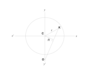
Figure 1: Geometry of the problem. O: observer, K: galaxy, C: cluster’s centre

2 Observed velocities

For the sake of simplicity, let us consider the $xy$ plane of a spherically symmetric cluster, undergoing a radial collapse (Fig.1), where $\@vec{r}$ is the position vector of a galaxy at K, relative to the centre C of the cluster. The velocity $\@vec{v}$ of the galaxy at K relative to the observer is given by the relation

$$\@vec{v}=\frac{\mathrm{d}\@vec{r}}{\mathrm{d}t}+\@vec{v}_{\mathrm{C}},\\$$ (1)

where $\@vec{v}_{\mathrm{C}}$ is the velocity of the centre C relative to O. Defining $v_{r}(r)=\mathrm{d}r/\mathrm{d}t$, where $r$ is the magnitude of $\@vec{r}$ and multiplying both sides of eqn.(1) by the unit vector $\hat{\@vec{r}}_{\mathrm{K}}$ along $\overrightarrow{OK}$ direction, we have

$$v_{\mathrm{obs}}(r,R)=\@vec{v}_{\mathrm{C}}\cdot\hat{\@vec{r}}_{\mathrm{K}}\pm\sqrt{1-\left({\frac{R}{r}}\right)^{2}}v_{r}(r),\\$$ (2)

where $v_{\mathrm{obs}}=\@vec{v}\cdot\hat{\@vec{r}}_{\mathrm{K}}$ is the observed velocity along the line–of–sight. From eqn.(2), for $r=R$ and for $r=r_{\mathrm{M}}$, the observed velocity takes the same value $v_{\mathrm{obs}}(r,R)=\@vec{v}_{\mathrm{C}}\cdot\hat{\@vec{r}}_{\mathrm{K}}$. Thus, $v_{\mathrm{obs}}$ takes extreme values for $r$ between $R$ and $r_{\mathrm{M}}$. We denote by $r_{\mathrm{M}}$ the radius of maximum expansion (turnaround radius) where $v_{r}(r_{\mathrm{M}})=0$.

For constant $R$, the quantity $\@vec{v}_{\mathrm{C}}\cdot\hat{\@vec{r}}_{\mathrm{K}}$ does not depend on $r$ and thus the condition $\partial v_{\mathrm{obs}}/\partial r=0$ for the extreme is written

$$\left[1-\left({\frac{R}{r}}\right)^{2}\right]\frac{\mathrm{d}v_{r}(r)}{\mathrm{d}r}+\frac{R^{2}}{r^{3}}v_{r}(r)=0.\\$$ (3)

The solution $r_{*}$ for $r$ of eqn.(3) is a function of $R$ ($r_{*}=r_{*}(R)$). This $r_{*}$ is the radial –relative to the centre of the cluster– distance of the galaxy which shows the observer the maximum or minimum velocity at a given $R$. Thus, the extreme values of $v_{\mathrm{obs}}$ at $R$ are

$$v_{\mathrm{obs,ext}}(R)=\@vec{v}_{\mathrm{C}}\cdot{\hat{\@vec{r}}}_{\mathrm{K}}\pm\sqrt{1-\left[{\frac{R}{r_{*}(R)}}\right]^{2}}v_{r}(r_{*}(R)).\\$$ (4)

The curves described by eqn.(4) are known as caustics (Regös & Geller (regos (1989))).

Following Diaferio et al. (diaf97 (1997)), we define the amplitude $A$ of the caustics by the relation

$$A(R)=\frac{1}{2}[v_{\mathrm{obs,max}}(R)-v_{\mathrm{obs,min}}(R)],$$ (5)

which is given by

$$A(R)=-\sqrt{1-\left({\frac{R}{r_{*}}}\right)^{2}}v_{r}(r_{*}).\$$ (6)

Note that by definition $v_{r}$ is negative in the infall region of the cluster. The amplitude contains only information about the dynamical situation of the cluster, since effects due to the motion of the observer relative to the cluster are excluded. Such effects are described by the term $\@vec{v}_{\mathrm{C}}\cdot\hat{\@vec{r}}_{\mathrm{K}}$ in eqn. (4) and have been studied by Praton & Schneider (praton (1994)). Differentiating eqn.(6) with respect to $R$, we have

$$\frac{\mathrm{d}A}{\mathrm{d}R}=\frac{Rv_{r}(r_{*})}{r_{*}^{2}\sqrt{1-\left({\frac{R}{r_{*}}}\right)^{2}}}$$

$$-\left[\frac{R^{2}v_{r}(r_{*})}{r_{*}^{3}\sqrt{1-\left({\frac{R}{r_{*}}}\right)^{2}}}+\sqrt{1-\left({\frac{R}{r_{*}}}\right)^{2}}\frac{\mathrm{d}v_{r}(r_{*})}{\mathrm{d}r_{*}}\right]\frac{\mathrm{d}r_{*}}{\mathrm{d}R}.$$ (7)

Because of eqn. (3), the term inside brackets equals zero and this leads to

$$\frac{v^{2}_{r}(r_{*})}{r_{*}^{2}}=-\frac{A(R)}{R}\frac{\mathrm{d}A(R)}{\mathrm{d}R}.\$$ (8)

Using eqns. (6) and  (8) we have

$$r_{*}=R\sqrt{1-\left(\frac{\mathrm{d}\ln A(R)}{\mathrm{d}\ln R}\right)^{-1}}.\$$ (9)

Solving eqn.(9) for $R$ and substituting in eqn.(8) the radial velocity is fully defined. This is an interesting result, since it shows that the exact data can give the exact profile of the infall velocity, in the case of a completely radial collapse. It is interesting to note that the above relations lead to eqn.(10), relating the logarithmic derivatives of the amplitude to the infall velocity;

$$\frac{\mathrm{d}\ln[-v_{r}(r_{*})]}{\mathrm{d}\ln r_{*}}=\frac{\mathrm{d}\ln A(R)}{\mathrm{d}\ln R}\$$ (10)

The above equations refer to the ideal case of a pure spherical collapse and completely accurate observations. In real systems, the velocity field is a superposition of a radial systematic component and a component of a random nature. The first one can be assumed as spherically symmetric while the second accounts for the effects of small-scale substructure and observational errors. The effects of small-scale substructure are clearly shown in the results of N-body simulations performed by van Haarlem and van de Weygaert (van (1993)). They conclude that the velocity profile, as predicted by the spherical infall model, compares badly with the actual velocity field resulting from their simulations. In real systems, such as the Coma cluster, the smearing of the form of the caustics is also clear (van Haarlem et.al vh (1993)). However, if the systematic radial component of the velocity field is known, a mass profile of the infall regions of the clusters can be determined, applying the spherical infall model. This profile should give a lower limit for the mass of the system since the effects of small-scale substructure reported above increase the amplitude of the caustics. Thus, we apply the previous eqns. assuming that $v_{r}$ describes the systematic radial component of the velocity. In Sect.4 we use model functions for the amplitude $A$, calculating the profile of $v_{r}$ by eqns. (8) and (9), we apply the spherical infall model and we derive a mass profile for the Coma cluster. These model functions for $A$ are smooth and decreasing, as it required by eqns. (8) and (9), and their approximation is based on the respective curves estimated by Geller et al. (gell99 (1999)).

3 The spherical infall model – Mass estimation

The eqn. of motion of a spherical shell of initial radius $a$ is given by Newton’s law as

$$\ddot{r}=\frac{\mathrm{d}^{2}r}{\mathrm{d}t^{2}}=-\frac{GM(r)}{r^{2}}$$ (11)

where $M(r)$ is the mass inside radius $r$ and $G$ is the gravitational constant. If the mass inside the shell is conserved (no shells crossing), then $M(r)$ is constant and equal to $M(a)$. We assume that this condition holds in what follows. Multiplying eqn.(11) by $\dot{r}$ and integrating, we have

$$\left(\frac{\mathrm{d}r}{\mathrm{d}t}\right)^{2}=v^{2}(t)=2E+\frac{2GM(a)}{r}$$ (12)

where $E={1}/{2}\leavevmode\nobreak\ {v_{i}}^{2}-(GM(a))/a$ is a constant with dimensions of specific energy and $v_{i}$ is the initial velocity. The solution of the above eqn., in the case of negative $E$, is given in parametric form by the expressions

$$r=\frac{GM(a)}{(-2E)}(1-cos\eta)\$$ (13)

$$t=\frac{GM(a)}{(-2E)^{\frac{3}{2}}}(\eta-sin\eta)+t_{a}.\$$ (14)

In order to synchronize all shells, we add the constant $t_{a}$ given by $t_{a}=t_{i}-\frac{GM(a)}{(-2E)^{\frac{3}{2}}}(\eta_{i}-\sin{\eta_{i}})$, where $t_{i}$ is the age of the universe at the initial conditions and $\eta_{i}$ is the initial phase of the shell, given by eqn.(13) for $r=a$. A shell reaches the radius of maximum expansion for $\eta=\pi$ and completes its collapse for $\eta=2\pi$. We denote by $\mu(a)$ the fractional excess of mass of a sphere of radius $a$, relative to the mass $M_{b}(a)$ of a sphere of the same radius that has a constant density (equal to the mean density of the universe at the initial conditions). Using the relation between the mean density of the universe $\rho_{b}$, the Hubble constant $H$ and the density parameter $\Omega$, that is

$$\rho_{b}(t)=\frac{3H^{2}(t)\Omega(t)}{8\pi G},$$ (15)

the mass inside radius $a$ is given by

$$M(a)=\frac{H^{2}_{i}\Omega_{i}a^{3}}{2G}(1+\mu(a)),\$$ (16)

where index $i$ stands for the values at the initial conditions. Assuming that the initial velocity of the shell is that of Hubble’s flow ($v_{i}=aH_{i}$), the energy $E$ is written

$$E=\frac{1}{2}H^{2}_{i}a^{2}\Omega_{i}\left[{\Omega_{i}}^{-1}-1-\mu(a)\right]\$$ (17)

Substituting eqn.(17) in eqns. (13), (14) and calculating the time derivative of the radius yields the relations

$$r=\frac{a}{2}\frac{{\mu_{e}(a)}+{\Omega_{i}}^{-1}}{\mu_{e}(a)}(1-\cos{\eta})\\$$ (18)

$$t=\frac{\mu_{e}(a)+{\Omega_{i}}^{-1}}{2H_{i}{\Omega_{i}}^{\frac{1}{2}}{\mu_{e}}^{\frac{3}{2}}(a)}(\eta-\sin{\eta})+t_{a}\\$$ (19)

$$v_{r}=aH_{i}{\Omega_{i}}^{\frac{1}{2}}{\mu_{e}}^{\frac{1}{2}}(a)\frac{\sin{\eta}}{1-\cos{\eta}}\\$$ (20)

where $\mu_{e}(a)=1+\mu(a)-\Omega_{i}^{-1}$.

Combining eqns. (18), (19) and (20) results in

$$(t-t_{a})\frac{v_{r}}{r}=\frac{\sin{\eta}(\eta-\sin{\eta})}{(1-\cos{\eta})^{2}},\\$$ (21)

where $t$ is the present age of the shell. The time $t$ is approximated by $t={H_{0}}^{-1}f(\Omega_{0},z)$, where $z$ is the redshift of the cluster, $H_{0}$ is the present value of the Hubble constant and $\Omega_{0}$ is the value of the density parameter. The function $f$ for the Friedmann-Lemaitre cosmological model is given in standard books of cosmology (see Zel’dovich & Novikov zeldovich (1983)) and its form depends on the value of $\Omega_{0}$ relative to the critical value $\Omega_{0}=1$. Reasonable initial conditions are those at the epoch of decoupling, when matter starts playing a significant role. The value of $t_{a}$ is very small compared to $t$, so it can be omitted without significant error in the calculation of the phase $\eta$. However, eqn. (21) can also be solved in its full form based on the following procedure. Solving eqn.(18) for $\mu_{e}$ gives

$$\mu_{e}(a)=\frac{a(1-\cos{\eta}){\Omega_{i}}^{-1}}{2r-a(1-\cos{\eta})}.$$ (22)

The substitution of the above expression in eqn.(20) leads to the following cubic for $a$

$$a^{3}+(1-\cos{\eta})^{2}Ca-2r(1-\cos\eta)C=0$$ (23)

where $C=v^{2}_{r}/(\sin^{2}{\eta}H^{2}_{i})$. This has one real and positive root, given by the relation

$$a=\left(\frac{rv^{2}_{r}}{H^{2}_{i}(1+\cos\eta)}\right)^{\frac{1}{3}}\left[(1+\sqrt{F})^{\frac{1}{3}}+(1-\sqrt{F})^{\frac{1}{3}}\right]$$ (24)

where

$$F=1+\frac{1}{r^{2}}\frac{(1-cos\eta)^{3}}{27}\frac{v^{2}_{r}}{H^{2}_{i}(1+\cos\eta)}.$$ (25)

Thus, $\mu_{e}$ can be expressed as a function of $r,v_{r},H_{i},\Omega_{i}$ and $\eta$. Then, $t_{a}$ can also be expressed in terms of the same variables, since it is given by the relation

$$t_{a}=t_{i}-\frac{1}{2H_{i}\Omega^{\frac{1}{2}}_{i}}\frac{\mu_{e}(a)+\Omega^{-1}_{i}}{\mu_{e}^{\frac{3}{2}}(a)}(\varphi-{\sin}^{-1}\varphi)$$ (26)

where $\varphi=\frac{2\mu^{\frac{1}{2}}_{e}(a)}{\Omega^{\frac{1}{2}}_{i}(\mu_{e}(a)+\Omega^{-1}_{i})}$ and $t_{i}$ is the age of the universe at the initial conditions (decoupling), given in standard books of cosmology (see Zel’dovich & Novikov zeldovich (1983)).

The present method can be summarized as follows: A known profile of the amplitude of the caustics, using eqns. (8) and (9) leads to the profile of radial velocity. Then, the solution of eqn.(21) defines the phase $\eta$ of any shell. Assuming no shell crossing during the evolution of the cluster, the combination of eqns. (16), (18) and (20) gives the mass inside a spherical region with current radius $r$ as

$$M(r)=\frac{r{v^{2}}_{r}}{G}\frac{1-\cos{\eta}}{sin^{2}\eta}.$$ (27)

4 Applications

The procedure described above is applied to estimate a lower limit for the mass profile of the Coma cluster. For this purpose, we employ data provided by Geller et al. (gell99 (1999)). The largest sample presented by these authors contains 691 galaxies. The cluster’s velocity $cz_{\mathrm{C}}$ ($c$ is the speed of light and $z_{\mathrm{C}}$ is the redshift of the cluster centre) is $7\,090\mathrm{Km\,sec^{-1}}$ and for a Hubble constant $H_{0}=100\mathrm{h\,Km\,sec^{-1}\,Mpc^{-1}}$, its distance is $70.9\mathrm{h^{-1}\,Mpc}$.

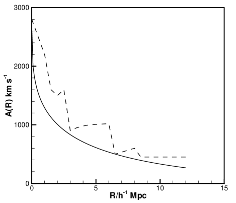
Figure 2: Dashed line: profile of the amplitude of the caustics (Geller et al. (gell99 (1999))). Solid curve: approximation of this line using analytical smooth functions (see eqn.(28) and text for more details.)

As noted in Sect. 2, our approach is based on the profile of the amplitude $A$ of the caustics. Departures from spherical symmetry, random motions due to the development of substructure, the finite number of galaxies in the cluster and observational errors are some of the reasons making the determination of caustics non-trivial. A general approach, given by Diaferio (diaf99 (1999)), is based on the argument that caustics are high density regions (see Regös & Geller regos (1989)) and is as follows. First, a smooth estimate for the density $f$ of observed galaxies on the $(R,v_{obs})$ plane is calculated and then a cut is applied at some density contour which is taken to correspond to the caustics. A similar procedure is followed by Reisenegger et al. (reinse (2000)) in their application to the Sharpley Supercluster. Problems associated with the above procedure, such as the choice of smoothing lengths and the density cutoff, are discussed in the above papers. The dashed line –shown in Fig. 2– is Geller et al.’s (gell99 (1999)) estimation of the amplitude $A_{est}(R)$ of the caustics derived by the above–discussed procedure. We assume that this can be written in the form

$$A_{est}(R)=A(R)+dA(R)$$

where $A(R)$ stands for the component due to the radial infall velocity and the positive $dA(R)$ describes the

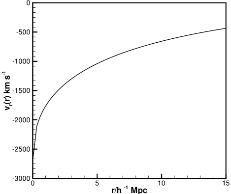
Figure 3: Radial velocity profile corresponding to the smooth curve plotted in Fig.2

’inflation’ of the caustics due to the development of random motions. Unfortunately, $dA(R)$ cannot be modelled properly and an infinite number of curves lower than $A_{est}$ could be provided as models for $A$. For this reason we use the following procedure. First, we use models for $A(R)$ of the form

$$A(R)=v_{0}\left[1-\left(\frac{R}{r_{\mathrm{M}}}\right)^{\frac{1}{k}}\right]^{k},\leavevmode\nobreak\ v_{0}\geq 0,\leavevmode\nobreak\ R\leq r_{\mathrm{M}}.$$ (28)

Then, we estimate the values of the parameters $v_{0},r_{M}$ and $k$ in order that these curves satisfy the condition $dA(R)>0$ for all values of $R$ and minimize the sum $\sum[A_{est}(R)-A(R)]^{2}$. In this way, we derive a profile that could be considered as an upper bound for the $A$ component. Such a curve is plotted in Fig.2. The parameters used in eqn.(28) are: $v_{0}=2\,700\mathrm{Km\,sec^{-1}},r_{\mathrm{M}}=60h^{-1}\mathrm{Mpc},k=2.8$. We note that $r_{\mathrm{M}}$ is not the physical radius of the system, but a fitting parameter. The form of eqn.(28) has mathematical advantages, since it allows an analytical evaluation of the profile of the infall velocity, using eqns. (8) and (9) reported in Sect. 2. This is given by the relation

$$v_{r}(r)=-v_{0}\left[1-\left(\frac{r}{r_{\mathrm{M}}}\right)^{\frac{2}{2k-1}}\right]^{k-{\frac{1}{2}}},\leavevmode\nobreak\ r\leq{r_{\mathrm{M}}},\leavevmode\nobreak\ k>{\frac{1}{2}}\$$ (29)

with $r=\left(\frac{r_{\mathrm{M}}}{R}\right)^{\frac{1}{2k}}R$.

In Fig.3, the resulting profile of the radial infall velocity is plotted. Assuming that the above profile is a good approximation of the radial systematic component of the infall velocity, we apply the spherical infall model to calculate mass profiles, for various values of the density parameter $\Omega_{0}$ of the universe, that are plotted in Fig.4. Starting from the bottom of the figure, the different curves correspond to $\Omega_{0}=0.2,0.4,0.6,0.8,1.0$ respectively. Larger values of $\Omega_{0}$ lead to steeper mass profiles at the outer regions. The variation of $\Omega_{0}$ alters the profile at the outer regions of the cluster and (as expected) larger values of the density parameter of the universe give rise to larger amount of mass inside a given radius. Notice that the mass scales as ${\Omega_{0}}^{0.2}$, roughly as expected (see Regös & Geller regos (1989)). Thus, the matter inside $10h^{-1}\mathrm{Mpc}$ varies for various values of the density parameter of the universe in the range $0.994$ to $1.12\times 10^{15}h^{-1}M_{\sun}$. The dashed curve, plotted also in this Fig., is the cumulative mass of an halo with a Navarro et al. (navarro (1995)) profile. This is given by the relation $M(r)=4\pi{\rho}_{0}{r^{3}}_{s}\{\ln[1+(r/rs)]-(r/rs)/[1+(r/rs)]\}$, where $\rho_{0}$ and $r_{s}$ are fitting parameters. The values of the parameters used are: $\rho_{0}=3.8\times 10^{15}h^{2}M_{\sun}\mathrm{Mpc}^{-3}$, $r_{s}=0.2h^{-1}\mathrm{Mpc}$. It is clearly shown in Fig.4 that there is a remarkable agreement of the form of the cumulative mass profiles estimated by the present approach (solid curves) with the Navarro et al. (navarro (1995)) mass profile (dashed curve). Note that the dashed curve describes the mass profile in the virialized region of the cluster.

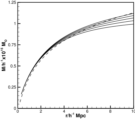
Figure 4: Mass profiles corresponding to the radial velocity profile (Fig.3) for varying $\Omega_{0}$. From the bottom of the figure, the curves correspond to $\Omega_{0}=0.2,0.4,0.6,0.8,1.0$ respectively. Dashed curve: Navarro et al. (navarro (1995)) mass profile.

5 Conclusions

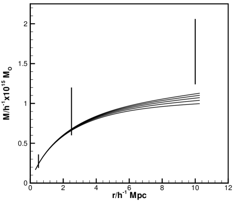
Figure 5: Mass profiles for various values of $\Omega_{0}$ as in Fig.4. The bar at $0.5$ shows the limits given by Hughes (hughes (1989)) while the bar at $2.5$ shows the limits given by Briel et al. (briel (1992)). The outer bar at $10$ shows the estimation given by Geller et al. (gell99 (1999))

Several methods have been proposed in the literature regarding the estimation of the mass of galaxy clusters.

A class of such methods, used to estimate the density profile of these systems, is based on the use of X-ray data (The & White the (1988); Hughes hughes (1989); Watt et al. watt (1992)). It is assumed that the gas is described by the equation of hydrostatic equilibrium. The latter is solved using the density and temperature profiles of the gas, that are measured using X-ray observations. This method is accurate in the region where the hydrostatic equilibrium holds, that is the central region of galaxy clusters. For example, Hughes (hughes (1989)) determined the minimum and maximum mass profiles consistent with all the data for Coma –if the mass-to-light ratio of the data was not constrained to be a constant– obtaining allowed mass ranges of $M_{0.5}=1.9-3.6\times 10^{14}h^{-1}M{\sun}$ and $M_{2.5}=0.5-1.5\times 10^{15}h^{-1}M{\sun}$ where $M_{0.5}$ and $M_{2.5}$ are the masses inside $0.5h^{-1}\mathrm{Mpc}$ and $2.5h^{-1}\mathrm{Mpc}$ respectively. Briel et. al (briel (1992)) used their ROSAT survey image to measure the X-ray surface brightness out to $100^{\prime}$ from the cluster center. They found that the binding mass is more centrally concentrated than the X-ray gas, and obtain $M_{2.5}=0.6-1.2\times 10^{15}h^{-1}M{\sun}$.

Another class of methods employs the projected velocities of the galaxies-members of the cluster. The methods based on the form of the caustics in redshift space belong -among others- in this class. In a series of papers (Diaferio et al. diaf97 (1997); Diaferio diaf99 (1999); Geller et al. gell99 (1999)), it has been proposed to estimate the mass profile of a galaxy cluster using the equation

$$GM(r)\approx\frac{1}{2}\int_{0}^{r}{A^{2}_{est}(x)\mathrm{d}x}.$$ (30)

Although there is no rigorous proof for this relation, its testing against cosmological N-body simulations shows that it approximates well the mass profiles. The derivation of the above relation is based on the argument that the amplitude of the velocity field of galaxy clusters depends mainly on local dynamics, since the random motion is significant. The mass profile is, in any case, roughly proportional to the square of the amplitude of the caustics and since the amplitude used by Geller at al. (gell99 (1999)) is larger because it includes the effect of random motion, one expects their estimation to result in a larger mass for the system. They estimate a mass inside a radius of $10h^{-1}\mathrm{Mpc}$ in the range $(1.65\pm 0.41)\times 10^{15}h^{-1}M_{\sun}$.

In Fig.5, we compare the mass estimations provided by our method for the Coma cluster to the mass estimations given by Hughes (hughes (1989)) , Briel (briel (1992)) and Geller et al. (gell99 (1999)). It is clear that the mass profile resulting from our application shows the minimum estimated values of mass at different radii and provides a reasonable estimation of the lower limit of the mass profile of the system.

More detailed observations could lead to a more accurate definition of the caustics and improve the estimation of mass profiles .

- (1) Briel, U.G., Henry, J.P. & Böhringer, H. 1992, A&A,259, L31
- (2) Diaferio, A. & Geller, M.J. 1997, ApJ 481, 633
- (3) Diaferio, A. 1999, MNRAS 309, 610
- (4) Geller, M. J., Diaferio, A. & Kurtz, M. J. 1999, ApJ 517, L23
- (5) Gunn, J. E. & Gott, J. R. 1972, ApJ 176, 1
- (6) Gunn, J. E. 1977, ApJ 218, 592
- (7) Hughes, J.P. 1989, ApJ 337,21
- (8) Kaiser, N. 1987, MNRAS 227, 1
- (9) Navarro, J. F., Frenk, C. S. & White, S. D. M. 1995, MNRAS 275, 720
- (10) Ostriker, E. C., Huchra, J. P., Geller, M. J., & Kurtz, M.J. 1988, AJ 96, 1775
- (11) Peebles, P. J. E. 1976, ApJ 205, 318
- (12) Peebles, P. J. E. 1980, The Large Scale Structure of the Universe (Princeton University Press, Princeton), 64
- (13) Praton, E. A. & Schneider, S. E. 1994, ApJ 422, 46
- (14) Regös, E. & Geller, M. J 1989, AJ 98, 755
- (15) Reinsenegger, A., Quintana, H., Carrasco, E. R., et al. 2000, AJ 120, 523
- (16) Schechter, P. L. 1980, AJ 85, 801
- (17) Shectman, S. A. 1982, ApJ 262, 9
- (18) Silk, J. 1974, ApJ 193, 525
- (19) The, L. S. & White, S. D. M. 1988, AJ 95, 15
- (20) van Haarlem, M. P. & van de Weygaert, R. 1993, ApJ, 418, 544
- (21) van Haarlem, M. P., Cayón, L., de la Cruz, C.G., et al. 1993 MNRAS 264, 71
- (22) Watt, M. P., Ponman, T.J., Bertram, D., et al. 1992, MNRAS 258, 738
- (23) Zel’dovich, Y. B. & Novikov, I. D. 1983, The Structure and Evolution of the Universe (The University of Chicago Press, Chicago and London), 54