On the reliability of peak-flux distributions, with an application to solar flares

Narrow-band radio spikes have been recorded during a solar flare with unprecedented resolution. This unique example allows us to study the effect of low resolution in previously published peak-flux distributions of radio spikes. We give a general, analytical expression for how an actual peak-flux distribution is changed in shape if the peaks are determined with low temporal and/or frequency resolution. It turns out that, generally, low resolution tends to cause an exponential behavior at large flux values if the actual distribution is of a power-law shape. The distribution may be severely altered if the burst-duration depends on the peak-flux. The derived expression is applicable also to peak-flux distributions derived at other wavelengths (e.g. soft and hard X-rays, EUV). We show that for the analyzed spike-event the resolution was sufficient for a reliable peak flux distribution. It can be fitted by generalized power-laws or by an exponential.

1 Introduction

Statistical flare models envisage the flare process as an ensemble of sub-processes and do not focus on the single constituent processes. The most prominent of these global models are the so-called Cellular Automaton models (Lu & Hamilton 1991; Lu et al. 1993; Vlahos et al. 1995; Georgoulis & Vlahos 1996; Galsgaard 1996; Georgoulis & Vlahos 1998; MacPherson & MacKinnon 1999; Isliker et al. 2000, 2001). They assume flares to be fragmented and stochastic processes, and so the need for a comparison through statistical quantities is present. Furthermore, there is direct evidence that flares are fragmented to some unknown level (deJager & deJonge 1978, Benz 1985, Aschwanden et al. 1990), and that flares really are stochastic processes (Isliker & Benz 1994; Isliker 1996; Ryabov et al. 1997, Veronig et al. 2000).

Observed peak-flux distributions of flares and flare fragments are used to test statistical flare models. Systems in a state of self-organized criticality (SOC) lack any characteristic scale and thus show power-law distributions. Stochastic growth in uncorrelated regions of instability yield log-normal peak-flux distributions found in interplanetary type III bursts (Cairns & Robinson 1997). Open driven plasmas yield burst-like pulses distributed exponentially at large fluxes (Robinson et al. 1996).

There exists a number of observational studies of peak-flux distributions of flare-related (non-thermal) emissions, in the hard X-ray range as well as in the radio range (see references in Aschwanden et al. 1998). In this article, we will concentrate on narrow-band, millisecond spike events in the radio range. Robinson et al. (1996) have determined a peak-flux distribution from a single-frequency spike observation, which they find to be exponential for high-flux values. Aschwanden et al. (1998) have analyzed some spike events with poor temporal resolution (typically one measurement point per spike event), and found exponential distributions. Mészárosová et al. (2000) analyzed single-frequency measurements of spikes. They found exponential and power-law distributions, the latter being very small in extent, however (much less than one decade). Such analyses raise a question: since every measurement is only at discrete points in time and frequency, a detected peak in an observation is in general not identical with the true peak which would be seen if continuous recording were feasible. The detected peak (termed pseudo-peak in the following) is likely to be further away from the true peak, the lower the time- and frequency-resolutions. Therefore the derived peak-flux distribution must be expected to be biased. Furthermore, peak-fluxes in the radio-range have mostly been determined at fixed frequencies, neglecting completely the fact that one may be far from the true peak in the frequency-direction. The question therefore is what bias in a peak-flux distribution must be expected due to finite and possibly low resolution in time and/or frequency.

We give an analytical expression of how a given true peak-flux distribution is changed when determined with finite time- and frequency-resolution (Sec. 2). The expression is independent of the wave-length range under consideration, it can also be applied e.g. to soft and hard X-rays, or to EUV. We then present the peak-flux distribution of narrow-band radio spikes in an event measured with unprecedented high time and frequency resolution (Sec. 3). We will discuss the peak-flux distribution of the spike event with the introduced statistical theory, as well as the distributions reported in the literature, which are subject to poor resolution, or even derived without frequency information. We will address the question of how good the time and frequency resolution must be (in terms of duration and bandwidth of the events), in order that the detected peak-flux distributions are near to the true ones, and what is to be expected if the frequency information is not available or not taken into account (Sec. 4).

2 The biasing of peak-flux distributions through finite resolution

In this section, we will establish the analytical expression which relates the peak-flux distribution of the true peaks to the distribution of the observed ones with given time and frequency resolutions, which we will refer to as pseudo-peaks. We start by making the following definitions:

Let $a$ be the amplitude of a pulse (e.g. spike), and assume a pulse-shape of the form

$$\Phi(\nu,t,a)=a\cdot\Phi_{\nu}(\nu\,g(a))\cdot\Phi_{t}(t\,h(a))\equiv a\cdot s$$ (1)

with $\Phi_{\nu}(0)=\Phi_{t}(0)=1$, and $g(a)$ and $h(a)$ functions of the amplitude $a$ (for instance $g(a)=1$, $a$, or $1/a$), and where we have introduced the abbreviation $s=s(\nu,t;a)$. Such a pulse-shape is reasonably general, but of course not completely so: we assume that the profiles in the frequency and in the time direction are independent, and particularly, it is assumed that the amplitude causes merely a scaling of the duration and/or bandwidth, and that there is no dependence on an additional, hidden, possibly stochastic parameter.

In statistical language, we consider the ideal measurement of the true peak-fluxes as the outcome of a random variable $A$, with probability density $p_{A}(a)$ ($a_{1}\leq a\leq a_{2}$) (which, in other words, is the normalized peak-flux distribution). Analogously, the measurement of pseudo peak-fluxes (the ones subject to finite temporal and spatial resolution) is considered as the outcome of a random variable $R$, with probability density $p_{R}(r)$. The question is what the relation between $p_{A}(a)$ and $p_{R}(r)$ is, i.e. we need to find the connection between $A$ and $R$:

Measuring the pseudo-peaks can be viewed as choosing a random point $(N,T)$ in the $\nu$-$t$-plane within a certain rectangle around the true peak, whose side-length are $\tau_{t}$ and $\tau_{\nu}$ (the temporal and spatial resolutions, respectively), and reading out the flux-value at this point. Hence, the uniform probability for choosing a random point $(N,T)$ in the rectangle of the $\nu$-$t$-plane is transformed into a probability distribution on the flux axis: for a given pulse with amplitude $A=a$, the random point $(N,T)$ transforms into a random point $a\cdot S$ on the flux axis through the pulse-shape, $a\cdot S\equiv a\cdot\Phi_{\nu}(N)\,\Phi_{t}(T)$, which will give the probability distribution $p_{S}(s)$ of the random variable $S$. More generally, we assume the pulse-shape to depend on the amplitude of the pulse (Eq. 1), so that S is given as

$$S=\Phi_{\nu}(N\cdot g(a))\cdot\Phi_{t}(T\cdot h(a)).$$ (2)

Its probability distribution is conditionally dependent on the amplitude, $p_{S}(s|a)$, and its range is $s_{1}(a)\leq S\leq s_{2}(a)\equiv 1$ ($p_{S}(s|a)\,ds$ denotes the conditional probability, i.e. the probability for $S$ to assume values in $[s,s+ds]$, given that $A$ is known to assume the value $a$). The random point on the flux-axis $a\cdot S$ is the pseudo-peak flux, so that the relation between the true and the pseudo peak-flux is, in terms of random variables,

$$R=A\cdot S$$ (3)

and the wanted pseudo-peak flux distribution $p_{R}(r)$ is given as

$$p_{R}(r)=p_{A\cdot S}(r).$$ (4)

Of course, it would be of interest to invert the problem, i.e. to derive from given $p_{R}(r)$ and $p_{S}(s)$ the true distribution $p_{A}(a)$. However, this is not possible, as will be shown in Sec. 2.4, since $p_{R}(r)$ and $p_{S}(s)$ do not contain enough information to uncover $p_{A}(a)$.

Three tasks are to be worked out now:

• The rectangle in the $\nu$-$t$-plane, out of which a random point is chosen, has to be determined (to find the probability density of the point $(N,T)$, which is needed to derive $p_{S}$ through Eq. 2).

• The probability $p_{S}(s|a)$ has to be derived (through Eq. 2), since it is an input to Eq. (4).

• The probability distribution of the product of the random variables $A$ and $S$ has to be found to evaluate Eq. (4), which yields the wanted $p_{R}$.

2.1 The rectangle around the true peak in which the pseudo-peak is located

The probability density $p_{N,T}(\nu,t)$ for the random point $(N,T)$ in the $\nu$-$t$-plane, at which the pseudo-peak flux is measured, is uniform in some region around the true peak (this follows from the complete absence of correlations between the measurement and the measured). In order to specify $p_{N,T}(\nu,t)$, the shape and size of this region have to be determined.

Without loss of generality, we may assume a true peak to occur at $t_{0}=0$, $\nu_{0}=0$. Since we assume the burst-profile to factorize (Eq. 1), we can expect the measurement point $(N,T)$ to lie in a rectangle,

$$(N,T)\in[L_{\nu-},L_{\nu+}]\times[L_{t-},L_{t+}]$$ (5)

around the true peak at $(t_{0},\nu_{0})=(0,0)$, and we may derive the time- and the frequency-interval independently. Note that we explicitly treat the case where the pulse-shape is asymmetric. If the pulse shape is symmetric, then the rectangle is simply given as $[-\tau_{\nu}/2,\tau_{\nu}/2]\times[-\tau_{t}/2,\tau_{t}/2]$, as follows straightforwardly from symmetry considerations.

We start with treating the time-direction. Assume a true peak to be located at $t_{0}=0$. In the measurement procedure, a grid of time-points $t_{i}$ is put onto the $t$-axis (with $t_{i}-t_{i-1}=\tau_{t}$, $\forall i$, with $\tau_{t}$ the time resolution), which is randomly positioned relative to $t_{0}=0$. At one of these points, say at $t_{i}$, the measured flux will be highest, and a pseudo-peak is detected. This means that (i) $a\Phi_{t}(t_{i})\geq a\Phi_{t}(t_{i}+\tau_{t})$, and (ii) $a\Phi_{t}(t_{i})\geq a\Phi_{t}(t_{i}-\tau_{t})$ (for now we assume the burst profile to be independent of the amplitude $a$). Obviously, the pseudo-peak occurance-time $t_{i}$ lies in the interval

$$t_{i}\in\Big{\{}t^{\prime}\Big{|}\Phi_{t}(t^{\prime})\geq\Phi(t^{\prime}+\tau_{t}),\ {\rm and} \ \Phi_{t}(t^{\prime})\geq\Phi_{t}(t^{\prime}-\tau_{t}),$$

$${\rm and} |t^{\prime}|\leq\tau_{t}\Big{\}}$$ (6)

The left boundary $L_{t-}$ is given by the equation $\Phi_{t}(L_{t-})=\Phi_{t}(L_{t-}+\tau_{t})$, with allowed values of $L_{t-}$ in $[-\tau_{t},0]$, and the right boundary $L_{t+}$ is analogously given by the equation $\Phi_{t}(L_{t+})=\Phi_{t}(L_{t+}-\tau_{t})$ in the range $L_{t+}\in[0,\tau_{t}]$. In order that these solutions are unique, we need to demand that the pulse-shape is convex ($\Phi_{t}^{\prime\prime}<0$), i.e. strictly increasing until the peak, and then strictly decreasing with time, which is reasonable for a pulse-shape. If $L_{t-}+\tau_{t}$ is inserted into the equation for $L_{t+}$, then it is seen that it solves this equation, whence

$$L_{t+}=L_{t-}+\tau_{t}$$ (7)

— the size of the interval out of which a random point is chosen in a measurement is $\tau_{t}$, the time-resolution. Of practical interest in the following will be that

$$\Phi_{t}(L_{t-})=\Phi_{t}(L_{t+}).$$ (8)

So far, we have omitted the scaling factors $h(a)$ and $g(a)$. $L_{t-}$, for instance, would actually have to be determined by the equation $\Phi_{t}(L_{t-}h(a))=\Phi_{t}((L_{t-}-\tau_{t})h(a))$ instead of the one above, and in general one expects the solution $L_{t-}$ to depend on $a$. Under quite general assumptions, however, $L_{t-}$ is independent of $a$, e.g. for Gaussian, exponential, or power-law pulse-shapes. All these examples are pulse-shapes with the general form $a\Phi_{t-}=a\phi_{0}(c+\phi_{-}(t\,h(a)))$ for the left branch, and $a\Phi_{t+}=a\phi_{0}(c+\phi_{+}(t\,h(a)))$ for the right branch, where $\phi_{0}$ is any invertible function (e.g. an exponential), $c$ a constant, and $\phi_{-}$ and $\phi_{+}$ may be different, but homogeneous of the same degree (i.e. $\phi_{i}(bt)=b^{\kappa}\phi_{i}(t)$, for $i=-,+$, and $\kappa$ a constant), e.g. a power-law.

Completely analogously, $L_{\nu+}$ and $L_{\nu-}$ are determined, and again $L_{\nu+}=L_{\nu-}+\tau_{\nu}$ ($\tau_{\nu}$ denotes the frequency resolution) and $\Phi_{\nu}(L_{\nu-})=\Phi_{\nu}(L_{\nu+})$ hold. With the determination of the rectangle in which the random point $(N,T)$ lies, the probability density $p_{N,T}$ follows immediately as

$$p_{N,T}(\nu,t)=p_{N}(\nu)p_{T}(t)={1\over\tau_{t}\tau_{\nu}},$$ (9)

since it is uniform, as explained at the beginning of this subsection.

2.2 The determination of $P_{S}(s|a)$

Instead of the probability density $p_{S}(s|a)$, we will derive the cumulative probability distribution $P_{S}(s|a):=\int_{s_{1}}^{s}p_{S}(s^{\prime}|a)\,ds^{\prime}$, since in general the density has a singularity at the peak ($s=1$) of the pulse. $P_{S}(s|a)$ is given implicitly by Eq. (2) as a function of the pulse-shape. Starting from the definition of $P_{S}(s|a)$ and inserting Eq. (2), we have

$$P_{S}(s|a) \equiv {\rm prob}\Big{[}S\leq s\,\Big{|}\,{\rm given\ that\ }A=a\Big{]}$$ (13)

$$= {\rm prob}\Big{[}\Phi_{\nu}(N\cdot g(a))\cdot\Phi_{t}(T\cdot h(a))\leq s\,\Big{|}\,a\Big{]}$$

$$= {\rm prob}\Big{[}(T,N)\in$$

$$\big{\{}(t,\nu)\,\big{|}\,\Phi_{\nu}(\nu\,g(a))\cdot\Phi_{t}(t\,h(a))\leq s,\ {\rm and}$$

$$\ L_{\nu-}\leq\nu\leq L_{\nu+},\ {\rm and}\ L_{t-}\leq t\leq L_{t+}\big{\}}\,\Big{|}\,a\Big{]}$$

$$= \int\!\!\!\!\!\!\!\!\!\!\!\!\!\!\!\!\!\!\!\!\!\!\!\!\!\!\!\!\!\!\!\!\int\limits_{\begin{array}[t]{c}\Phi_{\nu}(\nu\cdot g(a))\,\Phi_{t}(t\cdot h(a))\leq s\\ L_{\nu-}\leq\nu\leq L_{\nu+}\\ L_{t-}\leq t\leq L_{t+}\end{array}}\!\!\!\!\!\!\!\!\!\!\!\!\!\!\!\!\!\!\!\!\!\!\!\!\!\!\!\!\!\!\!\!p_{T}(t)\,p_{N}(\nu)\,dt\,d\nu$$

where $p_{T}(t)p_{N}(v)$ is given by Eq. (9).

Because of the possible asymmetry of the pulse-shape, it is necessary to treat the four quadrants separately. In each quadrant then, the integration limits in Eq. (10) imply four different cases, depending on the value of $s$. If in the four quadrants we denote the respective inverses of the pulse-shape by $\Phi_{t+}^{-1}$, $\Phi_{t-}^{-1}$, and $\Phi_{\nu+}^{-1}$, $\Phi_{\nu-}^{-1}$, and if we write $L_{t}$ where one can insert either $L_{t+}$ or $L_{t-}$ without changing the numerical values of the respective expressions (due to Eq. 8), and analogously $L_{\nu}$, then, in the first quadrant, we have (a substitution $\bar{t}:=\Phi_{\nu}(\nu)\Phi_{t}(t)$ allows to calculate the $t$-integral in Eq. 10):

• for $s\leq\Phi_{\nu}(L_{\nu}\,g(a))\,\Phi_{t}(L_{t}\,h(a))$

  $$P_{S}(s\,|\,a)=0$$ (14)

• for $\,\Phi_{\nu}(L_{\nu}\,g(a))\leq s$, and $\,\Phi_{t}(L_{t}\,h(a))\leq s$, and $s\leq 1$

  $$P_{S}(s\,|\,a) = \ {|L_{\nu+}L_{t+}|\over\tau_{\nu}\tau_{t}}$$

  $$- {1\over\tau_{\nu}\tau_{t}} \,{1\over g(a)}{1\over h(a)}\left|\int\limits_{0}^{\Phi_{\nu+}^{-1}(s)}\!\!\!d\nu\,\Phi_{t+}^{-1}\left({s\over\Phi_{\nu}(\nu)}\right)\right|$$ (15)

• for $\Phi_{\nu}(L_{\nu}\,g(a))\leq s\leq\Phi_{t}(L_{t}\,h(a))$

  $$P_{S}(s\,|\,a) = {|L_{\nu+}L_{t+}|\over\tau_{\nu}\tau_{t}}$$

  $$- {1\over\tau_{\nu}\tau_{t}} \,{1\over g(a)}{1\over h(a)}\left|\int\limits_{\Phi_{\nu+}^{-1}\left({s\over\Phi_{t}(L_{t}\,h(a))}\right)}^{\Phi_{\nu+}^{-1}(s)}\!\!\!\!\!\!\!\!\!\!\!\!\!\!\!d\nu\,\Phi_{t+}^{-1}\left({s\over\Phi_{\nu}(\nu)}\right)\right|$$ (16)

  $$- \left|{L_{t+}\over\tau_{\nu}\tau_{t}}\,\Phi_{\nu+}^{-1}\left({s\over\Phi_{t}(L_{t}\,h(a))}\right)\,{1\over g(a)}\right|$$

• for $\Phi_{t}(L_{t}\,h(a))\leq s\leq\Phi_{\nu}(L_{\nu}\,g(a))$

  $$P_{S}(s\,|\,a) = {|L_{\nu+}L_{t+}|\over\tau_{\nu}\tau_{t}}$$

  $$- {1\over\tau_{\nu}\tau_{t}} \,{1\over g(a)}{1\over h(a)}\left|\int\limits_{0}^{L_{\nu+}g(a)}\!\!\!d\nu\,\Phi_{t+}^{-1}\left({s\over\Phi_{\nu}(\nu)}\right)\right|$$ (17)

• for $\Phi_{\nu}(L_{\nu}\,g(a))\Phi_{t}(L_{t}\,h(a))\leq s$, and $s\leq\Phi_{\nu}(L_{\nu}\,g(a))$, and $s\leq\Phi_{t}(L_{t}\,h(a))$

  $$P_{S}(s\,|\,a) = {|L_{\nu+}L_{t+}|\over\tau_{\nu}\tau_{t}}$$ (18)

  $$-{1\over\tau_{\nu}\tau_{t}} \,{1\over g(a)}{1\over h(a)}\left|\int\limits_{\Phi_{\nu+}^{-1}\left({s\over\Phi_{t}(L_{t}\,h(a))}\right)}^{L_{\nu+}g(a)}\!\!\!\!\!\!\!\!\!\!\!\!\!\!\!d\nu\,\Phi_{t+}^{-1}\left({s\over\Phi_{\nu}(\nu)}\right)\right|$$

  $$- \left|{L_{t+}\over\tau_{\nu}\tau_{t}}\,\Phi_{\nu+}^{-1}\left({s\over\Phi_{t}(L_{t}\,h(a))}\right)\,{1\over g(a)}\right|$$

• for $1\leq s$

  $$P_{S}(s\,|\,a)={|L_{\nu+}L_{t+}|\over\tau_{\nu}\tau_{t}}$$ (19)

The non-trivial cases are for intermediate ranges of $s$, i.e. for $\Phi_{\nu}(L_{\nu}g(a))\Phi_{t}(L_{t}h(a))\leq s\leq 1$. The formulae for the other three quadrants are gained completely analogously to the given ones, by just correspondingly interchanging the indices $t+$, $t-$, $\nu+$, $\nu-$ (it is for this purpose that we had to write absolute values for all the appearing terms). If the pulse-shape is symmetric in $\nu$ and $t$, then the contributions of the four quadrants are equal.

2.3 The probability distribution of the product $A\cdot S$

In the last step, we determine the probability distribution $p_{R}$ of the pseudo-peaks, i.e. the probability distribution of the product $A\cdot S$ (Eqs. 3 and 4). The case of multiplying two random variables which are independent and have infinite range is found in standard textbooks. However, since both, $A$ and $S$, have finite range, and since $S$ is conditionally dependent on $A$, it is worthwhile to give the respective formulae. Essentially, the probability distribution of the product $A\cdot S$ equals $p_{A,S}(a,s)$, integrated over the subregion of the region $[a_{1},a_{2}]\times[s_{1}(a),s_{2}(a)]$ where $as\leq r$ is fulfilled ($p_{A,S}(a,s)$ is the joint probability distribution of $A$ and $S$). Using that $p_{A,S}(a,s)=p_{A}(a)p_{S}(s|a)$, we explicitly have

$$P_{R}(r) \equiv {\rm prob}[R\leq r]={\rm prob}[A\cdot S\leq r]$$ (23)

$$= \int\!\!\!\!\!\!\!\!\!\!\!\!\!\!\!\!\!\!\!\!\!\!\!\!\int\limits_{\begin{array}[t]{c}as\leq r\\ a_{1}\leq a\leq a_{2}\\ s_{1}(a)\leq s\leq s_{2}(a)\end{array}}\!\!\!\!\!\!\!\!\!\!p_{A,S}(a,s)\,da\,ds$$

$$= \int\limits_{\begin{array}[t]{c}a_{1}\leq a\leq a_{2}\\ a\leq r/s_{1}(a)\end{array}}\!\!\!\!\!\!\!\!\!\!p_{A}(a)\,da\int\limits_{\begin{array}[t]{c}s_{1}(a)\leq s\leq s_{2}(a)\\ s\leq r/a\end{array}}\!\!\!\!\!\!\!\!\!\!\!\!\!\!\!p_{S}(s\,|\,a)\,ds$$ (28)

where $s_{1}a_{1}\leq r\leq s_{2}a_{2}$. (As mentioned in Sec. 2.2, $p_{S}(s|a)$ might have a singularity at $s=1$, and we must therefore use the cumulative probability distribution $P_{S}(s|a)$, which is achieved if also for $R$ we use the cumulative probability distribution $P_{R}(r)$, as done in Eq. (17), and identify $\int_{\alpha}^{\beta}p_{S}(s^{\prime}|a)\,ds^{\prime}=P_{S}(\beta|a)-P_{S}(\alpha|a)$.)

In the following, we write again $L_{t}$ if inserting $L_{t+}$ or $L_{t-}$ does not change the respective numerical values, and correspondingly $L_{\nu}$ is used instead of $L_{\nu+}$ or $L_{\nu-}$. For intermediate values of $r$, i.e. for $a_{1}\cdot\Phi_{\nu}(L_{\nu}g(a_{1}))\Phi_{t}(L_{t}h(a_{1}))\leq r\leq a_{2}$, four non-trivial cases of integration limits turn out to exist, depending on the values of r. We have:

• for $r\leq a_{1}\cdot\Phi_{\nu}(L_{\nu}\,g(a_{1}))\,\Phi_{t}(L_{t}\,h(a_{1}))$

  $$P_{R}(r)=0$$ (29)

• for $r\leq a_{2}\cdot\Phi_{\nu}(L_{\nu}\,g(a_{2}))\,\Phi_{t}(L_{t}\,h(a_{2}))$, and $r\leq a_{1}$

  $$P_{R}(r)=\!\!\!\!\!\!\!\!\!\!\int\limits_{a_{1}}^{a\leq r/\Phi_{\nu}(L_{\nu}\,g(a))\,\Phi_{t}(L_{t}\,h(a))}\!\!\!\!\!\!\!\!\!\!\!\!\!\!\!da\,p_{A}(a)\,P_{S}(r/a\,|\,a)$$ (30)

• for $a_{1}\leq r\leq a_{2}\cdot\Phi_{\nu}(L_{\nu}\,g(a_{2}))\,\Phi_{t}(L_{t}\,h(a_{2}))$

  $$P_{R}(r)=P_{A}(r)\,+\!\!\!\!\!\!\!\!\!\!\!\!\!\!\!\int\limits_{r}^{a\leq r/\Phi_{\nu}(L_{\nu}\,g(a))\,\Phi_{t}(L_{t}\,h(a))}\!\!\!\!\!\!\!\!\!\!\!\!\!\!\!\!\!\!\!\!da\,p_{A}(a)\,P_{S}(r/a\,|\,a)$$ (31)

• for $a_{2}\cdot\Phi_{\nu}(L_{\nu}\,g(a_{2}))\,\Phi_{t}(L_{t}\,h(a_{2}))\leq r\leq a_{1}$

  $$P_{R}(r)=\int\limits_{a_{1}}^{a_{2}}da\,p_{A}(a)\,P_{S}(r/a\,|\,a)$$ (32)

• for $a_{2}\cdot\Phi_{\nu}(L_{\nu}\,g(a_{2}))\,\Phi_{t}(L_{t}\,h(a_{2}))\leq r$, and $a_{1}\leq r$, and $r\leq a_{2}$

  $$P_{R}(r)=P_{A}(r)+\int\limits_{r}^{a_{2}}da\,p_{A}(a)\,P_{S}(r/a\,|\,a)$$ (33)

• for $a_{2}\leq r$

  $$P_{R}(r)=1$$ (34)

Inserting $P_{S}(s|a)$ (Eqs. (11) to (16)) into the formulae for $P_{R}(r)$ yields the desired pseudo peak-flux distribution.

2.4 Inversion is not possible

To derive the true peak flux distribution from a given pseudo-peak flux distribution (the inverse problem), we have to proceed as follows: from Eq. (3) we find

$$A=R/S,$$ (35)

and we can uncover the true distribution from the pseudo one analogously as we had proceeded in Eq. (17):

$$P_{A}(a) \equiv {\rm prob}[A\leq a]={\rm prob}[R/S\leq a]$$ (36)

$$= \int\!\!\!\!\!\!\int\limits_{r/s\leq a}p_{R,S}(r,s)\,dr\,ds$$

$$= \int\!\!\!\!\!\!\int\limits_{r/s\leq a}p_{R}(r|s)p_{S}(s)\,dr\,ds$$

so that we need to know the conditional probability $p_{R}(r|s)$ of $R$ given that $S$ is known. That $R$ is not independent of $S$ is evident from the fact that $R$ is equivalent to $A\cdot S$, and one explicitly finds, if $p_{A}(a)$ is assumed to be known, that

$$P_{R}(r|s)=P_{A}(r/s)$$ (37)

What is measured, however, is

$$p_{R}(r)=\int\limits_{s_{1}\leq s\leq s_{2}}p_{R}(r|s)p_{S}(s)\,ds,$$ (38)

the distribution of $R$ irrespective of the value of $S$, so that all the conditional information is lost. In other words, to uncover $P_{A}(a)$ one has to know $P_{R}(r|s)$, which is essentially equivalent to knowing the true peak-flux distribution $P_{A}(a)$ (see Eq. 26), and which would be feasible only in continuous observations. Whence it follows that uncovering the true distribution from the measured one is not possible.

3 The peak-flux distribution of solar narrow-band spikes

Table 1: Fits of different functional forms to the peak-flux distributions of the event 1982/06/04 (see Sec. 3), where the four data-sets are distributions derived from a) peaks in 2D plane, $\tau_{t}=2\,{\rm ms}$, $\tau_{\nu}=1\,{\rm MHz}$ (data-set a); b) peaks at $\nu=362\,{\rm MHz}$, $\tau_{t}=2\,{\rm ms}$ (data-set b); c) peaks in 2D plane, $\tau_{t}=100\,{\rm ms}$, $\tau_{\nu}=1\,{\rm MHz}$ (data-set c); d) peaks at $\nu=362\,{\rm MHz}$, $\tau_{t}=100\,{\rm ms}$ (data-set d). If the $\chi^{2}$ approved a fit, then the power-law index or an ’o.k.’ is stated, else a ’—’ is noted.

data	nr. of	$ax^{c}$	$a(x-b)^{c}$	$a(x-b)^{c}+d$	$ae^{cx}$
set	peaks	$c=$	$c=$	$c=$
a	59	—	-15.6$\pm$6.8	-2.7$\pm$7.5	o.k.
b	144	—	—	-14.9$\pm$7.3	o.k.
c	38	-1.2$\pm$0.2	-3.5$\pm$6.9	-0.8$\pm$7.9	o.k.
d	76	—	-16.3$\pm$4.8	-15.8$\pm$6.8	o.k.

The solar narrow-band millisecond spike event we analyzed was observed by the ETH Zurich radio-spectrometer on 1982/06/04, 13:38:41 UT (the event is published and described in Güdel & Benz, 1990; Csillaghy & Benz, 1993). The resolution is 2 ms in time and 1 MHz in frequency (from 361 to 364 MHz), whereas the spikes have a typical duration of 73 ms (FWHM; Güdel & Benz, 1990), and a typical bandwidth of 7 MHz (FWHM; Csillaghy & Benz, 1993). Hence the spikes are well resolved in time. Also in frequency, the spikes are resolved although the observation range (4 MHz) is smaller than the typical bandwidth, as only spikes with peaks unambiguously in the range are taken into account. The peaks were determined by looking for strong enough local maxima above the noise-level, and a constant background was subtracted (representing the quiet Sun). The normalized distribution of the respective peak-fluxes is shown in Fig. 1 (solid line, with error-bars).

Different curves were fitted to this distribution, and a $\chi^{2}$-test was performed to check whether the fits are compatible with the data or not. The fitted curves are: a simple power-law ($ax^{c}$), two generalized forms of power-laws ($a(x-b)^{c}$, and $a(x-b)^{c}+d$), and an exponential ($ae^{x}$). The result is presented in Fig. 2 and summarized in Table 1 (data-set a): The peak-flux distribution of the event can be fitted by the generalized power-laws as well as by the exponential, but not by the simple power-law. The indices of the generalized power-laws are subject to large errors (determined by the bootstrap resampling method) due to the large error-bars (the number of peaks is relatively small) and due to the relative flexibility of the generalized power-laws (three resp. four free parameters and 10 data-points).

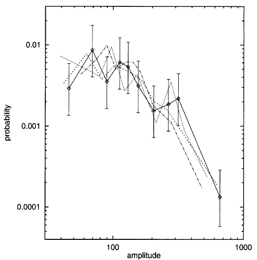
Figure 1: Peak-flux distributions (probability densities) of the narrow-band spike event 1982/06/04 (see Sec. 3): a) peaks in 2D plane, $\tau_{t}=2\,{\rm ms}$, $\tau_{\nu}=1\,{\rm MHz}$ (solid line, with error- bars); b) peaks at $\nu=362\,{\rm MHz}$, $\tau_{t}=2\,{\rm ms}$ (dashed line); c) peaks in 2D plane, $\tau_{t}=100\,{\rm ms}$, $\tau_{\nu}=1\,{\rm MHz}$ (dotted line); d) peaks at $\nu=362\,{\rm MHz}$, $\tau_{t}=100\,{\rm ms}$ (dash-dotted line). (The histograms are drawn by connecting the midpoints of the bins, and the bin-widths are such that each contains the same number of data-points. The amplitude is in SFU.)

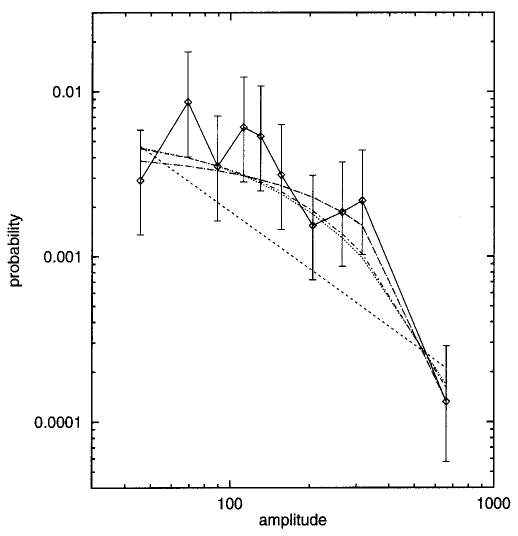
Figure 2: Fits to the peak-flux distribution (probability density) of the narrow-band spike event 1982/06/04 (see Sec. 3, and also Table 1). The peaks are determined in the 2D plane, with $\tau_{t}=2\,{\rm ms}$ and $\tau_{\nu}=1\,{\rm MHz}$. Plotted are the original data (solid line), and the fits $ax^{c}$ (dashed), $a(x-b)^{c}$ (dotted), $a(x-b)^{c}+d$ (dash-dotted), $ae^{x}$ (wide dash-dotted). (The histogram is drawn and generated as described in Fig. 1, and the amplitude units are again SFU.)

4 Discussion of the empirical peak-flux distributions

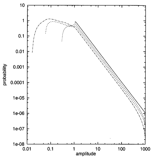
Figure 3: Amplitude-independent pulse-shape: (0) True peak-flux distribution ($\alpha=2$, $a_{1}=1$, $g(a)=h(a)\equiv 1$) (solid), together with the pseudo peak-flux distributions for (i) $\tau_{t}=2\,{\rm ms}$, $\tau_{\nu}=1\,{\rm MHz}$ (dashes); (ii) $\tau_{t}=2\,{\rm ms}$, $\tau_{\nu}=15\,{\rm MHz}$ (small dashes); (iii) $\tau_{t}=100\,{\rm ms}$, $\tau_{\nu}=1\,{\rm MHz}$ (dots); (iv) $\tau_{t}=100\,{\rm ms}$, $\tau_{\nu}=15\,{\rm MHz}$ (dot-dashed). The cases (0) and (i) practically coincide.

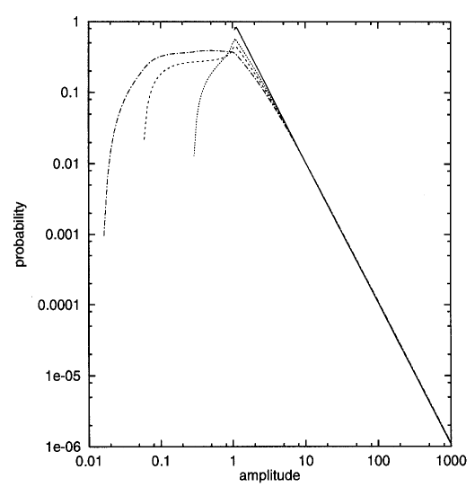
Figure 4: Amplitude-dependent pulse-shape I: True peak-flux distribution ($\alpha=2$, $a_{1}=1$, $g(a)=h(a)=a^{-1}$) (solid), together with pseudo peak-flux distributions for $\tau_{t}$ and $\tau_{\nu}$ as described in the caption to Fig. 3. The cases (0) and (i) practically coincide.

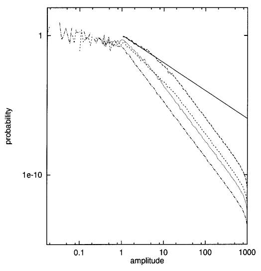
Figure 5: Amplitude-dependent pulse-shape II: True peak-flux distribution ($\alpha=2$, $a_{1}=1$, $g(a)=h(a)=a^{1}$) (solid), together with pseudo peak-flux distributions for $\tau_{t}$ and $\tau_{\nu}$ as described in the caption to Fig. 3.

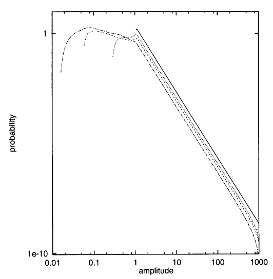
Figure 6: Steeper true distribution: True peak-flux distribution ($\alpha=3$, $a_{1}=1$, $g(a)=h(a)\equiv 1$) (solid), together with pseudo peak-flux distributions for $\tau_{t}$ and $\tau_{\nu}$ as described in the caption to Fig. 3. The cases (0) and (i) practically coincide.

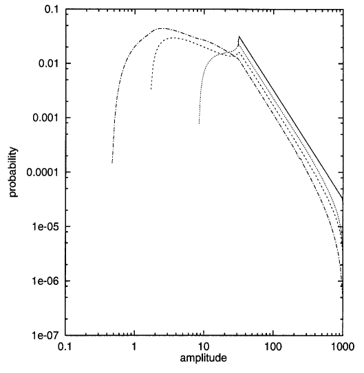
Figure 7: Smaller range of amplitudes: True peak-flux distribution ($\alpha=2$, $a_{1}=30$, $g(a)=h(a)\equiv 1$) (solid), together with pseudo peak-flux distributions for $\tau_{t}$ and $\tau_{\nu}$ as described in the caption to Fig. 3. The cases (0) and (i) practically coincide.

To apply the statistical theory introduced in Sec. 2 to the narrow-band spike event analyzed in Sec. 3, we have to make an assumption about the pulse-shape of the individual spikes. According to Güdel & Benz (1990), and Csillaghy & Benz (1993), it is reasonable to assume a Gaussian pulse-shape, i.e.

$$\Phi_{\nu}(\nu)=e^{-{1\over 2}\left({\nu\over b_{\nu}}\right)^{2}}$$ (39)

and

$$\Phi_{t}(t)=e^{-{1\over 2}\left({t\over b_{t}}\right)^{2}}$$ (40)

with $b_{\nu}=3.1\,{\rm MHz}$, and $b_{t}=31\,{\rm ms}$ (implying a FWHM of $7.3\,{\rm MHz}$, and $73\,{\rm ms}$, respectively, as reported by Güdel and Benz (1990), and Csillaghy and Benz (1993) for the given event). Furthermore, we have to assume a distribution of the true peak-fluxes $A$: we let $p_{A}(a)$ be a straight power-law

$$p_{A}(a)=Ca^{-\alpha},\ \ \ a_{1}\leq a\leq a_{2}$$ (41)

with $a_{2}=1000$ (from Fig. 1). Other true distributions can be expected to produce qualitatively the same effects as reported below for the case of this power-law.

The crucial parameters are the time-resolution $\tau_{t}$ and the frequency-resolution $\tau_{\nu}$, they determine how near the pseudo-peaks are to the true-peaks, on average. Whence, in the following parametric study (Figs. 3 to 7), we always show the true peak-flux distribution $p_{A}(a)$, together with the pseudo peak-flux distributions for four cases of time- and frequency-resolution: (i) good resolution in time and frequency, (ii) good resolution in time and a bad one in frequency, (iii) bad resolution in time and a good one in frequency, and (iv) bad resolution in both time and frequency (by ’good’ we mean $\tau<<$ FWHM, and ’bad’ means $\tau=2$ FWHM). The cases (ii) and (iv) represent also the case of single-frequency observations.

First, we investigate the case of an amplitude-independent pulse-shape, i.e. $g(a)=h(a)\equiv 1$ (see Eq. 1), and we set $a_{1}=1$, $\alpha=2$. Fig. 3 shows that for good resolution both in frequency and time the true and the pseudo peak-flux distributions practically coincide. If one or both resolutions are low, then the pseudo-peak flux distribution is generally near the true one, with a faster fall-off at high flux-values, however, i.e. a turning from power-law to exponential behaviour. At pseudo peak-flux values smaller than $a_{1}$, a completely artificial, relatively flat extension of the distribution appears. Turn-overs at small fluxes in distributions detected with low resolution(s) might thus be just the effect of an intrinsic low-amplitude cut-off in the true fluxes. Only high resolution analysis can tell whether or not such a flattening is real or not. The turning-over effect increases if the resolution decreases.

We turn now to the case of amplitude dependent pulse-shapes. If we let $g(a)=h(a)=a^{-1}$, then we get a deviation from the power-law behavior at small flux values, but nice coincidence for intermediate and high values (Fig. 4). For $g(a)=h(a)=a^{1}$ the slope (and shape at high flux-values) is drastically changed to a stronger fall-off (Fig. 5), the observed distribution is different even for good time and frequency resolution.

The general behavior demonstrated so far is rather independent of the shape of the original, true peak-flux distribution: In Fig. 6, we let again $g(a)=h(a)\equiv 1$, but now the power-law index $\alpha=3$. The corresponding pseudo peak-flux distributions behave analogously to the case $\alpha=2$ (Fig. 3).

It is worthwhile noting that the parameter $a_{1}$ may enhance the effect of turning to exponential behavior at high flux values: in Fig. 7, we let $g(a)=h(a)\equiv 1$ and $\alpha=2$, as in Fig. 3, but $a_{1}=30$ (cf. the lower cut-off in Fig. 1), and the tendency seen in Fig. 3 is enhanced, now. Thus, we conclude that the roll-over at large amplitude is more serious for a small range of amplitudes.

Obviously, it is crucial to know whether the durations and bandwidths of the pulses depend on the amplitude: Csillaghy and Benz (1993) report that the bandwidth of spikes sometimes is correlated with the amplitude, sometimes it is not, and sometimes it is anti-correlated. There is, however, no generally holding strong tendency, so that we may assume that the peak-flux distribution reported in Sec. 3 is near the true one.

This is also confirmed by the following: we artificially worsened the time and the frequency resolution in the data of Sec. 3 and compared the respective histograms: The dashed line in Fig. 1 is the histogram of the pseudo-peak fluxes resulting if the frequency information is completely neglected, i.e. one of the frequencies is selected, and the peaks are determined as maxima in time-direction only. The dotted line is the distribution for the resampled observation, using only every 50th data-point in time, which yields a spectrogram with $0.1\,{\rm sec}$ time resolution, and keeping full frequency resolution. Finally, the dashed-dotted line is the distribution for the resampled data, with again fixing a frequency and neglecting completely the corresponding information. Obviously, the biasing effects are smaller than the statistical errors in the distributions, all four distributions coincide within the error-bars, and the results are fairly independent of the sampling — only the fits seem to show different kinds of behavior (Table 1), but, as mentioned, the indices of the generalized power-laws are subject to large errors. The relative robustness (within the statistical errors) of the distribution on under-sampling is in turn a signature for amplitude-independent pulse-shapes.

5 Conclusion

The statistical theory we introduced allows us to predict the deviation of a pseudo-peak flux distribution from the true peak-flux distribution if the time and frequency resolutions are known. It turns out that in general there is a tendency towards exponential behavior at large flux values; the more expressed, the lower the resolutions are, including in particular the case of single-frequency observations. Only with high resolutions in both frequency and time (compared e.g. to the respective FWHM) are the detected distributions reliable in the whole range. The dependence of the pulse-shape on the amplitude (peak-flux) is crucial: If the width of a pulse (duration or bandwidth) is proportional to the inverse of the amplitude, then a strong deviation from the true peak flux distribution will result, the distributions will be steepened and completely biased in the whole range, even for high resolution in both frequency and time. If the width of the pulse is directly proportional to the amplitude, then a bias (flattening) appears only in the low amplitude range. All the biasing effects get stronger with a smaller extent of a distribution.

A different possible cause for a strong bias at low amplitudes (appearance of a relatively flat part in the detected distribution) is a possible intrinsic lower cut-off of the true amplitudes. Only high resolution data analysis can make sure whether a flattening at low amplitudes is real or an artifact.

The example of a narrow-band spike event we analyzed is a unique observation with respect to the high temporal and frequency resolutions; the spikes are completely resolved in frequency and time. Since moreover the burst-width seems to depend at most slightly on the amplitude, we conclude on the basis of our analytical study that the peak-flux distribution we get is reliable. It can be fitted by generalized power-laws or by an exponential, but definitely not by a simple power-law.

From our analysis, it follows that the peak-flux distributions of spikes reported by Robinson et al. (1996), Aschwanden et al. (1998), and Mészárosová et al. (2000), though observed with poor time-resolution or without any frequency information, are near the true distributions, except for the high-flux part, which must be expected to be too steep.

The exponential distribution we find supports the open driven plasma model (Robinson et al. 1996). We did though not try to fit a log-normal distribution, which in view of the relatively large statistical error in the empirical distribution, is likely to be also accepted by the $\chi^{2}$-test, so that we cannot exclude the stochastic growth theory (Cairns & Robinson 1997).

Conclusions on whether the distribution we find is compatible or not with SOC models are more difficult to draw. SOC models are models for the primary energy release, so far they do not include a mechanism for radio- (plasma-) emission. Moreover, the peak-fluxes of SOC models, which have been analyzed statistically, are defined as the peak-fluxes of entire flares, whereas here and in the cited articles on radio observations, the peak-fluxes of all the flare-fragments are analyzed. For both reasons, a direct comparison of SOC models to radio data is not possible without substantial new developments.

The statistical theory introduced here can be applied to the peak-flux distributions of all the different kinds of bursts, independent of the wavelength at which they occur, as soon as the pulse-shape and the functional dependency of the pulse-shape on the amplitude are (at least approximately) known: to radio-bursts (recent empirical studies include Aschwanden et al. (1998; type III, decimetric pulsations), Mercier and Trottet (1997; type I)), to soft X-rays, EUV, hard X-rays, etc. (see e.g. the review of Crosby et al. 1993; Krucker & Benz 1998).

- (1) Aschwanden, M.J., Benz, A.O., Schwartz, R.A., Lin, R.P., Pelling, R.M., Stehling, W., 1990, Solar Phys. 130, 39
- (2) Aschwanden, M.J., Dennis, B.R., Benz, A.O., 1998, ApJ 497, 972
- (3) Benz, A.O., 1985, Solar Phys. 96, 357
- (4) Cairns, I.H., Robinson, P.A., 1997, Geophysical Research Lett. 24 (No. 4), 369
- (5) Crosby, N.B., Aschwanden, M.J., Dennis, B.R., 1993, Solar Phys. 143, 275
- (6) Csillaghy, A., Benz, A.O., 1993, A&A 274, 487
- (7) Galsgaard, K., 1996, A&A 315, 312
- (8) Georgoulis, M., Vlahos, L., 1996, ApJ 469, L135
- (9) Georgoulis, M., Vlahos, L., 1998, A&A 336, 721
- (10) Güdel, M., Benz, A.O., 1990, A&A 231, 202
- (11) Isliker, H., 1996, A&A 310, 672
- (12) Isliker, H., Anastasiadis, A., Vlahos, L., 2000, A&A 363, 1134
- (13) Isliker, H., Anastasiadis, A., Vlahos, L., 2001, A&A, submitted
- (14) Isliker, H., Benz, A.O., 1994, A&A 285, 663
- (15) deJager, C., deJonge, G., 1978, Solar Phys. 58, 127
- (16) Krucker, S., Benz, A.O., 1998, ApJ 501, L213
- (17) Lu, E. T., Hamilton, R. J., 1991, ApJ 380, L89
- (18) Lu, E. T., Hamilton, R. J., McTierman, J. M., Bromund, K.R., 1993, ApJ 412, 841
- (19) MacPherson, K.P., MacKinnon, A.L., 1999, A&A 350, 1040
- (20) Mercier, C., Trottet, G., 1997, ApJ 474, L65
- (21) Mészárosová, H., Karlicky, M., Veronig, A., Zlobec, P., Messerotti, M., 2000, A&A 360, 1126
- (22) Robinson, P.A., Smith, H.B., Winglee, R.M., 1996, Phys. Rev. Lett. 76 (No. 19), 3558
- (23) Ryabov, V.B., Stepanov, A.V., Usik, P.V., Vavriv, D.M., Vinogradov, V.V., Yurovsky, Yu.F., 1997, A&A 324, 750
- (24) Veronig, A., Messerotti, M., Hanslmeier, A., 2000, A&A 357, 337
- (25) Vlahos, L., Georgoulis, M., Kluiving, R., Paschos, P., 1995, A&A 299, 897