Constraining Cosmological Parameters Based on Relative Galaxy Ages

Abstract

We propose to use relative galaxy ages as a means of constraining cosmological parameters. By measuring the age difference between two ensembles of passively–evolving galaxies at somewhat different redshifts, one could determine the derivative of redshift with respect to cosmic time, $dz/dt$. At high redshifts, $z\sim 1$–$2$, this measurement would constrain the equation-of-state of the dark energy, while at low redshifts, $z\lesssim 0.2$, it would determine the Hubble constant, $H_{0}$. The selected galaxies need to be passively–evolving on a time much longer than their age difference.

1 Introduction

Recently, there has been much progress in constraining cosmological parameters, such as the matter content of the Universe (Peacock et al. 2001) and the Hubble constant (Freedman et al. 2001). Available data for the microwave background anisotropies on degree scales (de Bernardis et al. 2000; Hanany et al. 2000; Netterfield et al. 2001; Lee et al. 2001 ) and the Hubble diagram of Type Ia supernovae (Riess et al. 1998; Perlmutter et al. 1999) indicate that the Universe has a flat geometry and is dominated at present by some form of dark energy with a negative pressure (Garnavich et al. 1998; Perlmutter et al. 1999). The equation of state of the dark energy, $p_{Q}=w_{Q}\rho_{Q}$, expresses the ratio between the pressure, $p_{Q}$, and the mass density, $\rho_{Q}$, of the dark energy in terms of the parameter $w_{Q}$ (in units of $c=1$). The value of $w_{Q}$ could either be constant as in the case of a cosmological constant ($w_{Q}=-1$), or time-dependent as in the case of a rolling scalar field or “Quintessence” (Ratra & Peebles 1988; Caldwell et al. 1998). Any such behavior would have far–reaching implications for particle physics. Therefore, the next observational challenge is to determine the evolution of $w_{Q}$ as a function of redshift (Huterer & Turner 2000; Maor et al. 2001; Weller & Albrecht 2001). The related observations need to be done at redshifts $z\lesssim 2$, when the dark energy started to dominate the expansion of the Universe.

The popular approach for measuring $w_{Q}(z)$ uses its effect on the luminosity distance of sources. In particular, the proposal for the Supernova/Acceleration Probe (SNAP) mission suggests to monitor $\lesssim 2000$ Type Ia supernovae across the sky per year and determine their luminosity distances up to a redshift $z\sim 1.5$ with high precision. However, the sensitivity of the luminosity distance to the redshift history of $w_{Q}(z)$ is compromised by its integral nature (Maor et al. 2001),

$$d_{\rm L}=(1+z)\int_{z}^{0}(1+z^{\prime}){dt\over dz^{\prime}}dz^{\prime},$$ (1)

where $t(z)$ is the age of the Universe at a redshift $z$ which depends on $w_{Q}(z)$.

In this paper, we propose an alternative method that offers a much better sensitivity to $w_{Q}(z)$ since it measures the integrand of equation (1) directly. Any such method must rely on a clock that dates the variation in the age of the Universe with redshift. The clock in our method is provided by spectroscopic dating of galaxy ages. Based on measurements of the age difference, $\Delta t$, between two passively–evolving galaxies that formed at the same time but are separated by a small redshift interval $\Delta z$, one can infer the derivative, $(dz/dt)$, from the ratio $(\Delta z/\Delta t)$. The statistical significance of the measurement can be improved by selecting fair samples of passively–evolving galaxies at the two redshifts and by comparing the upper cut-off in their age distributions. All selected galaxies need to have similar metallicities and low star formation rates (i.e. a red color), so that the average age of their stars would far exceed the age difference between the two galaxy samples, $\Delta t$.

This differential age method is much more reliable than a method based on an absolute age determination for galaxies (e.g., Dunlop et al. 1996; Alcaniz & Lima 2001; Stockton 2001). As demonstrated in the case of globular clusters, absolute stellar ages are more vulnerable to systematic uncertainties than relative ages (Stetson, Vandenberg & Bolte 1996). Moreover, absolute galaxy ages can only provide a lower limit to the age of the Universe and only place weak constraints on the possible histories of $w_{Q}(z)$.

The quantity measured in our method is directly related to the Hubble parameter,

$$H(z)=-{1\over(1+z)}{dz\over dt}.$$ (2)

Hence, an application of this method to old elliptical galaxies in the local Universe can be used to determine the value of the current Hubble constant, $H_{0}$.

In §2 we quantify the advantage of the above differential age method relative to the standard luminosity distance method in constraining the history of $w_{Q}(z)$. We then describe the spectroscopic dating technique and apply it to mock galaxy spectra in §3. In particular, we analyze the dependence of the cosmological constraints on the signal-to-noise ratio of the spectroscopic data and the number of observed galaxies. The significance level of the constraints attainable with a single pair of galaxies, dictates the number of such pairs required in order to differentiate between various histories of $w_{Q}(z)$. Finally, we summarize our main conclusions in §4.

2 Observables

We consider a flat universe composed of matter and dark energy, the latter having an equation of state $p_{Q}=w_{Q}(z)\rho_{Q}$, where $w_{Q}$ may depend on redshift. The Hubble parameter is $H^{2}=H_{0}^{2}[\rho_{T}(z)/\rho_{T}(0)]$. Here, the subscripts $Q$, $m$, and $T$ refer to the dark energy, the matter, or the total sum of the two, respectively. Assuming further that the matter is non-relativistic (i.e. effectively presureless), we get

$$H_{0}^{-1}{dz\over dt}=-(1+z){H(z)\over H_{0}}=-(1+z)^{5/2}\left[\Omega_{m}(0)+\Omega_{Q}(0)\exp\left\{3\int_{0}^{z}\frac{dz^{\prime}}{(1+z^{\prime})}w_{Q}\right\}\right]^{1/2},$$ (3)

where we have used the energy conservation equation for the dark energy, $\dot{\rho}_{Q}=-3H(1+w_{Q})\rho_{Q}$ (Maor et al. 2000). Thus, $({dz}/{dt})$ is related to the equation of state of the dark energy through one integration only, while the luminosity distance in equation (1) is given by an integral of the inverse of equation (3), namely through two integrations. By differentiating $(dz/dt)$ with respect to $t$ we find,

$$H_{0}^{-2}\frac{d^{2}z}{dt^{2}}=\frac{[H_{0}^{-1}({dz}/{dt})]^{2}}{(1+z)}\left[\frac{5}{2}+\frac{3}{2}w_{Q}(z)\right]-\frac{3}{2}\Omega_{m}(0)(1+z)^{4}w_{Q}(z),$$ (4)

which depends explicitly on $w_{Q}$ without any integrations. Thus, the second derivative of redshift with respect to cosmic time measures $w_{Q}$ directly. While it is possible to find significantly different redshift histories of $w_{Q}$ for which the evolution of $d_{\rm L}$ is similar, this cannot be done for $({d^{2}z}/{dt^{2}})$.

Maor et al. (2000) have argued that due to its integral form, the luminosity distance has only a weak discriminating power with respect to different possible histories of $w_{Q}(z)$. To demonstrate their case, they considered examples of $w_{Q}$ which have a quadratic dependence on $z$. Figure 1 shows similar examples (top panel) along with their corresponding observables, namely the luminosity distance $d_{\rm L}(z)$ (second panel), ${dz}/{dt}$ (third panel), and ${d^{2}z}/{dt^{2}}$ (bottom panel). The different $w_{Q}(z)$ histories generate a variation of $\sim 5\%$ in $d_{\rm L}$, $\sim 10\%$ in $({dz}/{dt})$, and $\sim 30\%$ in $({d^{2}z}/{dt^{2}})$ at $z\sim 1.5$. The last observable has a fractional variation as large as that of $w_{Q}(z)$.

3 Spectroscopic Dating of Passively–Evolving Gallaxies

The change of cosmic time with redshift may be inferred from the aging of stellar populations in galaxies. This inference must be done with caution since galaxies are vigorous sites of star formation at high redshift. It might seem difficult to estimate accurately the differential aging of the universe based on star–forming galaxies, since the stars in these galaxies are born continuously and a young stellar population may dominate their emission spectrum. Fortunately, examples of passively–evolving galaxies have already been identified in large numbers at high redshifts (Dunlop 1996; Daddi, Cimatti & Renzini 2000; Dey et al. 2001; Stockton 2001). We focus our attention on these red galaxies since their light is dominated by an old stellar population.

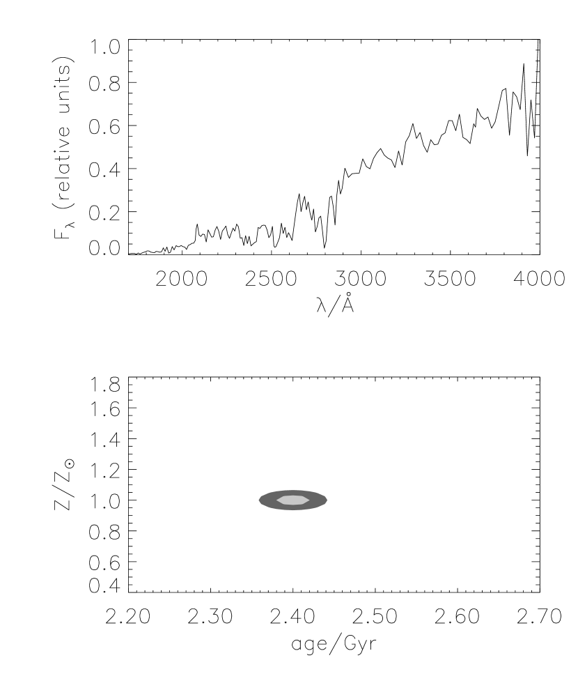
Figure 2: The top panel shows a simulated spectrum (flux per unit wavelength, $F_{\lambda}$) for a galaxy with a solar metallicity and an age of 2.4 Gyr, including Poisson photon noise with $S/N=30$ at a spectral resolution of 10Å. The bottom panel shows the accuracy of the metallicity and age recovery for $S/N=30$ (dark shaded region) and $S/N=50$ (lightly shaded region).

Our goal is to measure the age difference between two passively–evolving galaxies at different redshifts. How accurately can this be done? We emphasize that the relative age is better determined than the absolute age since systematic effects on the absolute scale are factored out (for a fractional age difference $\ll 1$). At redshifts $z\sim 1$–$2$ the rest-frame UV spectrum of non star–forming (elliptical) galaxies is dominated by light from main sequence stars with masses of 1–2 M_⊙, in a regime of stellar evolution that is well understood (Spinrad et al. 1997). The lack of interstellar dust or gas simplifies further the spectrum of old elliptical galaxies. The top panel in Figure 2 shows a simulated galaxy spectrum in the rest frame UV that can be easily collected by 10 meter class telescopes from the ground (e.g. Dunlop et al. 1996). This spectrum was calculated for a single stellar population with a specific metallicity (solar) and age (2.4 Gyr), using the synthetic stellar population models developed in Jimenez et al. (1998). The simulated spectrum has a 10 Å resolution, to which we have added Poisson photon noise with a signal-to-noise ratio $S/N=30$ per resolution element. The bottom panel shows the values recovered at the 95% confidence level (using a $\chi^{2}$ goodness-of-fit statistics) for the metallicity and age with $S/N=30$ (dark shaded region) and $S/N=50$ (lightly shaded inner region). Note that age and metallicity are not degenerate in the rest–frame UV, provided that the measured spectra have a sufficient $S/N$ (Nolan et al. 2001). A value of $S/N=15$–$30$ can be obtained for a faint galaxy of magnitude 24 in the $R$–band after 10 hours of integration on the Keck telescope (K. Adelberger, private communication). Observation of a sufficiently wide field of view would allow to measure spectra of many passively–evolving galaxies at the same time.

The assumption that stars in an elliptical galaxy have a single metallicity value is clearly an over-simplification. Local ellipticals have metallicity gradients (e.g. Davies et al. 1993), even though these gradients are mild (e.g. Friaca & Terlevich 1998). We therefore consider the possibility that elliptical galaxies have a mixture of populations with different metallicities. In order to assess the accuracy by which we can recover the age of a mixed stellar population, we simulated several spectra with a mixture of six metallicity values ranging from 0.01 to 5 times the solar value. For example, one of our models had weights of 5, 10, 25, 20, 12 and 28% for metallicities of 0.01, 0.2, 1, 2.5 and 5 times the solar value, respectively. We then attempted to recover the age by searching for the best–fit model with a single metallicity, and found an age uncertainty of 0.1 Gyr. Alternatively, we fitted the simulated spectrum by a mixed metallicity model with six free components, and recovered a more accurate age with an uncertainty of $\sim 0.05$ Gyr (as well as a reduced metallicity uncertainty of 8%).

Using the more conservative age uncertainty of 0.1 Gyr derived above for $S/N=30$, we may now estimate the attainable constraints on $w_{Q}(z)$ for a fiducial pair of passively–evolving galaxies which formed at the same time but are observed at $z=1.4$ and 1.6 and have ages of 2.79 and 2.4 Gyr, respectively. Figure 3 shows the resulting error bar on $(dz/dt)$, which is not sufficiently restrictive for a single pair of galaxies. However, for a statistical ensemble of independent galaxies (which do not all belong to the same local region of a galaxy cluster, for example), the error bar will be reduced by the square root of the number of analyzed galaxy pairs. The smaller error bar in the plot illustrates the constraint that could be placed by 20 such pairs. This constraint is sufficient to distinguish among the different $w_{Q}(z)$ histories in Figure 1.

The situation in reality is not as simple as described above, since a galaxy survey will not just identify galaxies that formed at the same cosmic time. Rather, the galaxies selected as not having substantial star formation, will show an age distribution at any given redshift. Given this age distribution, what is the accuracy by which one may recover the age shift, provided that the age of each passively–evolving galaxy is measured with a 0.1 Gyr uncertainty? To answer this question, we have simulated the galaxy age distributions at two different redshifts. The distribution at the higher redshift was modeled fiducially as a Schechter function which is asymptotically flat at low ages and is fully truncated at some finite maximum age value (because galaxies cannot be older than the age of the universe). In our example we chose a cutoff at 2.4 Gyr. The distribution was then binned into bins of 0.1 Gyr width, corresponding to the age uncertainty for individual galaxies. The age distribution at a lower redshift was chosen to be the same as the first one but shifted by either 0.0, 0.15 or 0.30 Gyr (so that the maximum age in the distribution would be 2.4, 2.55 or 2.7 Gyr, respectively). We also removed or added a fixed fraction (20%) of the galaxies within each bin through a random Poisson realization of this fraction. This degree of freedom is required since some galaxies may have merged with a star–forming galaxy and therefore disappeared from the old galaxy population. Moreover, the normalization of the two distributions is regarded as a free parameter because the volume surveyed at the two redshifts might be different. Our approach assumes that both samples of galaxies have been passively evolving for a time much longer than the age difference between the two redshifts. Each member of the low–redshift sample has a progenitor which, statistically speaking, is included in the high–redshift sample. But each high–redshift galaxy has some probability of encountering a merger and disappearing from the low–redshift sample. Our method would fail only if this probability is both significantly large and significantly age–dependent. However, for a sufficiently narrow redshift interval, the merger probability is small. The tight color–magnitude relation of present-day ellipticals further limits the effect of mergers on their age distribution (Peacock 1991; Bower, Lucey & Ellis 1992; Peacock et al. 1998).

The two distributions are shown as the two upper panels of Figure 4 for an age shift of 0.3 Gyr and a total of $\sim 75$ galaxies in each distribution. We binned the distributions for illustrative purposes. The best statistical method to recover the shift is the Kolmogorov–Smirnov (KS) test on the unbinned data. The bottom panel shows the probability for getting a particular value of the peak in the KS probability (Press et al. 1992) for the three cases we consider. We derived this probability distribution through a large number of Monte–Carlo realizations of the above distributions. Also shown as shaded regions are the shift levels for which one could distinguish among the different $w_{Q}(z)$ histories in Figure 3. We find that the shifts can be recovered with good precision, despite the fact that the tip of the age distribution is populated by a small number of galaxies. In particular, we get a $\gtrsim 90\%$ probability in this example for distinguishing among the different $w_{Q}(z)$ histories.

At present, there is no such set of galaxy spectra that could discriminate between a constant and a variable $w_{Q}(z)$. Nevertheless, it is instructive to examine the best spectroscopically observed pair of red galaxies to date, namely 53W091 and 53W069, which reside at $z=1.43$ and 1.55, respectively. The stellar populations of these galaxies have been studied in detail recently by Nolan et al. (2001), who demonstrated that the age–metallicity degeneracy can be broken based on UV rest-frame spectroscopy with high quality. However, since these galaxies where observed with only $(S/N)\sim 6$–$10$, they do not provide strong constraints on $w_{Q}(z)$.

4 Conclusions

We have shown that the derivative of cosmic time with respect to redshift can be used as an effective tool for measuring the equation of state of the dark energy as a function of redshift. For this purpose, spectra of passively–evolving galaxies need to be obtained with a high signal-to-noise ratio. In order to differentiate at the 2-$\sigma$ level between a constant and a variable $w_{Q}(z)$, one needs $\sim 70$ pairs of galaxies at $R\sim 24$. For a field of view $\sim(10^{\prime})^{2}$, which is attainable with instruments like DEIMOS on the Keck telescope and VIMOS on the VLT, we estimate that the required number of ellipticals may be found in the volume between $z=1.4$ and 1.6, and so all pairs can be observed simultaneously over 10 hours of integration on a 10 meter class telescope, such as Keck or the VLT.

The key advantages of our method relative to supernova searches such as the SNAP space mission, are that (i) the observable $(dz/dt)$ is more sensitive to $w_{Q}(z)$ than the luminosity distance $d_{\rm L}$; and (ii) the related precision observations can be done from the ground. In fact, some observational groups have already identified relevant sets of red galaxies at high–redshifts (e.g., Daddi et al. 2000; Stockton 2001).

The Hubble constant, $H_{0}$, can be measured by computing the age difference between red galaxies at $z=0$ and $z\sim 0.2$. The characteristic age difference in this redshift range, $\sim 2$ Gyr, can be measured for a single pair of galaxies with a precision of $\sim 20\%$ given data with $S/N=10$ and spectral resolution of 10Å . A large volume of spectroscopic data with this quality on red galaxies in the local universe, will soon be released by the Sloan Digital Sky Survey (SDSS). The wavelength coverage of the SDSS spectra of 3900–9100 Å  includes spectroscopic features such as $H_{\beta}$, that are sensitive to the aging of the stellar population. Given a statistical sample of many hundreds of red SDSS galaxies (D. Eisenstein, private communication), one could in principle determine the value of $H_{0}$ to a percent accuracy, as long as the systematic modeling uncertainties for relative ages can be reduced to that level. The differential age method is independent of the Cepheid distance scale and is subject to other uncertainties.

Figure 1: Several examples of $w_{Q}(z)$ as a function of redshift (top panel) and the sensitivity of several observables: $d_{\rm L}$ (second panel), $dz/dt$ (third panel) and $d^{2}z/dt^{2}$ (bottom panel).

Figure 3: The large error bar illustrates the constraint that can be placed on $w_{Q}(z)$ by using only a single pair of red galaxies that formed at the same time and are observed at $z=1.6$ and $z=1.4$. The spectra are assumed to have a spectral resolution of 10Å  and $S/N=30$. When data for 20 such pairs is available, the uncertainty is reduced to the thicker, smaller error bar.

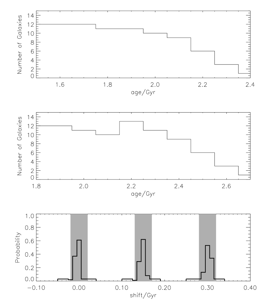
Figure 4: The top panel shows a hypothetical age distribution for 75 galaxies at a redshift $z=1.6$. The middle panel shows the same distribution at $z=1.4$, in which all galaxies are older by 0.3 Gyr and their fraction per bin changes by $\pm 20\%$ with Poisson fluctuations (due to mergers). The bottom panel shows the probability distribution of the recovered shift in age between the two galaxy distributions using the peak probability value of the KS–likelihood test for unbinned data with an age error of 0.1 Gyr per galaxy. We show three cases of shifts, namely: 0.0, 0.15 and 0.3 Gyr. The shaded regions show the range in the recovered shift which would allow to separate the different $w_{Q}(z)$ histories in Figure 3.

References

- Alcaniz & Lima (2001) Alcaniz, J. S. & Lima, J. A. S. 2001, ApJ, 550, L133
- (2) Bower, R. G., Lucey, J. R., Ellis R. S. 1992, MNRAS, 254, 601
- Caldwell, Dave, & Steinhardt (1998) Caldwell, R. R., Dave, R., & Steinhardt, P. J. 1998, Ap&SS, 261, 303
- de Bernardis et al. (2000) de Bernardis, P. et al. 2000, Nature, 404, 955
- (5) Daddi, E., Cimatti, A., Renzini, A. 2000, A&A, 362, 45
- (6) Dey et al. 2001, in preparation
- Dunlop et al. (1996) Dunlop, J., Peacock, J., Spinrad, H., Dey, A., Jimenez, R., Stern, D., & Windhorst, R. 1996, Nature, 381, 581
- Freedman et al. (2000) Freedman, W. L. et al. 2001, ApJ, in press; astro-ph/0012376
- Garnavich et al. (1998) Garnavich, P. M. et al. 1998, ApJ, 509, 74
- Hanany et al. (2000) Hanany, S. et al. 2000, ApJ, 545, L5
- Huterer & Turner (2000) Huterer, D. & Turner, M. S. 2000, Phys. Rev. D, submitted; astro-ph/0012510
- (12) Jimenez, R. Padoan, P. Matteucci, F. & Heavens, A. F. 1998, MNRAS, 299, 123
- (13) Lee, A.T. et al. 2001; astro-ph/0104459
- (14) Maor, I., Brustein, R., & Steinhardt, P. J. 2001, Phys. Rev. Lett. 86, 6
- (15) Netterfield, B. et al. 2001; astro-ph/0104460
- (16) Nolan, L. A., Dunlop, J. S., Jimenez, R., & Heavens, A. F. 2001, MNRAS, submitted; astro-ph/0103450
- (17) Peacock, J. A. 1991, in Blanchard A., Celnekier L., Lachieze–Rey, M., Tran Thanh Van J., eds, Proc. 2nd Rencontre de Blois, Physical Cosmology. Editions Frontieres, Gif-sur Yvette, p.337
- (18) Peacock, J. A. et al. 1998, MNRAS, 296, 1089
- (19) Peacock, J. A. et al. 2001; astro-ph/0103143
- Perlmutter et al. (1999) Perlmutter, S. et al. 1999, ApJ, 517, 565
- Perlmutter, Turner, & White (1999) Perlmutter, S., Turner, M. S., & White, M. 1999, Physical Review Letters, 83, 670
- (22) Press, W. H., Teukolsky, S. A., Vetterling, W. T., Flannery, B. P. 1992, Numerical Recipes. The art of scientific computing. Cambridge University Press.
- Ratra & Peebles (1988) Ratra, B. & Peebles, P. J. E. 1988, Phys. Rev. D, 37, 3406
- Riess et al. (1998) Riess, A. G. et al. 1998, AJ, 116, 1009
- (25) Spinrad, H. et al. 1997, ApJ, 484, 581
- (26) Stetson, P. B., Vandenberg, D. A., & Bolte, M. 1996, PASP, 108, 560
- (27) Stockton, A. 2001, to be published in Astrophysical Ages and Time Scales, ASP Conference Series; astro-ph/0104191
- (28) Weller, J. & Albrecht, A. 2001, Phys. Rev. Lett., 86, 1939