Future supernovae observations as a probe of dark energy

Abstract

We study the potential impact of improved future supernovae data on our understanding of the dark energy problem. We carefully examine the relative utility of different fitting functions that can be used to parameterize the dark energy models, and provide concrete reasons why a particular choice (based on a parameterization of the equation of state) is better in almost all cases. We discuss the details of a representative sample of dark energy models and show how future supernova observations could distinguish among these. As a specific example, we consider the proposed “SNAP” satellite which is planned to observe around 2000 supernovae. We show how a SNAP-class data set taken alone would be a powerful discriminator among a family of models that would be approximated by a constant equation of state for the most recent epoch of cosmic expansion. We show how this family includes most of the dark energy models proposed so far. We then show how an independent measurement of $\Omega_{\rm m}$ can allow SNAP to probe the evolution of the equation of state as well, allowing further discrimination among a larger class of proposed dark energy models. We study the impact of the satellite design parameters on this method to distinguish the models and compare SNAP to alternative measurements. We establish that if we exploit the full precision of SNAP it provides a very powerful probe.

I Introduction

One of the most challenging problems in modern cosmology is to provide an explanation for the recently observed accelerated expansion of the universe[1, 2, 3]. These observations have reopened the quest for the cosmological constant which was introduced by Einstein[4], but later abandoned[5] and infamously cited as his greatest blunder[6]. The cosmological constant can be considered as new kind of “world matter”[7] and be identified with the energy density of the vacuum[8], explaining and computing it in terms of particle physics has been largely unsuccessful[9, 10] because it is very difficult to explain the small vacuum energy density of $10^{-120}M_{\rm Pl}^{4}$ within fundamental physics; typically it is either much larger or exactly zero.

In recent years, the type Ia supernovae (SNe) as standard candles have been used to measure the distance-redshift relation in the universe providing evidence for an energy component in the universe which behaves like a cosmological constant[1, 2, 3]. This means the pressure of this component is negative and it appears to be dark in a sense that it is not recognizable by direct observation[11]. The Supernovae Cosmology Project (SCP)[1, 3] found evidence for a positive cosmological constant on the 99% level. These findings seem to be confirmed if one combines the most recent cosmic microwave background (CMB) radiation data from the BOOMERanG (Balloon Observations of Millimetric Extragalactic Radiation and Geomagnetics)[12, 13, 14, 15], MAXIMA (Millimeter Anisotropy eXperiment IMaging Array)[16, 17, 18] and DASI (Degree Angular Scale Interferometer)[19, 20] experiments with observations of rich clusters [21, 22].

With these observations we need a deeper understanding of the cosmological constant and attempts have been made to explain the missing energy as the energy density in a scalar field, which only interacts with the other fields via gravity. This field is rolling slowly down a potential or gets trapped in a local minimum[23, 24, 25, 26, 27, 28, 29, 30, 31, 32, 33, 34, 35, 36, 37, 38, 39, 40]. Therefore the vacuum energy of the universe becomes important for its evolution and the expansion begins to accelerate, generalizing the concept of the cosmological constant. Attempts have been made to connect this field to fundamental physics[29, 38] and resolve the problem of fine tuning of initial conditions[36]. The problem is that there is a plethora of models which can describe the observed expansion, but with the current available data it is not possible to distinguish between most of them.

To improve the observational situation a satellite mission – the “SuperNovae Acceleration Probe” (SNAP) –[41] and other dedicated SNe surveys have been proposed [42]. This satellite may observe about $2000$ SNe within two years and therefore increase the number of SNe by a factor of $25$. In this paper we present the details of a representative sample of dark energy models, discuss how the use of SNe as standard candles can distinguish the different models and what can be established about the equation of state of the dark energy component. Current upper bounds from SNe observations on the equation of state are $w_{\phi}\leq-0.6$ [11, 43, 45]. In order to reconstruct not only the constant contribution to the equation of state it is convenient to fit the SNe magnitude - redshift relation with a continuous function [44, 45, 46, 47, 86, 87, 88].

The main purpose of this paper is twofold: First we compare the quality of two different fits to the luminosity distance – redshift relation, where we emphasize the importance of a “good” fit in order to draw conclusion about the quality of the experiment. Secondly we analyze how SNe observations can constrain the equation of state factor and content of dark energy in the universe. A whole section presents the different dark energy models which we use for this analysis.

The outline of the paper is as follows. In section II we describe the current situation of the SNe observations, in section III we describe briefly the specifics of the proposed SNAP satellite mission, in section IV we introduce the commonly studied dark energy models, the parameters we choose for them and their cosmological evolution. In section V we discuss how to reconstruct the equation of state by expanding the equation of state factor as a power series in redshift and fit for the expansion coefficients. In section VI we discuss the impact of the experimental design and prior constraints on the matter content. Finally, section VII presents alternative measurements, before we draw our conclusions in VIII.

II The current observational situation

In this paper we concentrate on the results of the distant type Ia SNe observations [1, 2, 3] and mention other indications just briefly. The SCP and the High-Z Search Team used bright type Ia SNe as standard candles. These objects are thought to be thermonuclear explosions of carbon-oxide white dwarfs[50, 51, 52]. The correlation between the peak luminosity and the decline rate of the luminosity of the SNe[53, 54, 55, 56] makes it possible to estimate its magnitude and with spectral information about the host one can determine its redshift. The correlation can be quantified by the drop in magnitude $15$ days after the peak luminosity is reached. The SNe observations by the SCP are calibrated using the “low” redshift Calán/Tololo survey[57] which revealed that they have an excellent distance precision of $\sigma_{\rm mag}=0.15\;{\rm mag}$ for the magnitude and therefore can, in fact, be used as standard candles.

The apparent bolometric magnitude is given by

$$m(z)=M+5\log d_{\rm L}(z)+25\,,$$ (1)

with $M$ the absolute bolometric magnitude and $d_{\rm L}$ the luminosity distance, which is usually defined with distances in units of $10{\rm pc}$. However, cosmological distances are measured in ${\rm Mpc}$ and therefore there is an additional term $5\log{10^{5}}=25$ in eqn. (1). Furthermore, the luminosity distance depends on the cosmological evolution and hence on the cosmological parameters and is defined by $d_{\rm L}^{2}={\cal L}/4\pi{\cal F}$, where ${\cal F}$ is the measured flux and ${\cal L}$ the absolute luminosity of the object. The luminosity distance $d_{\rm L}$ can be expressed in terms of the coordinate distance $d_{\rm L}(z)=(1+z)r(z)$. As mentioned before the CMB data of BOOMERanG, MAXIMA and DASI[12, 13, 14, 15, 16, 17, 18, 19, 20] in combination with 2dF observations [58] indicates strongly that the universe has a flat topology and therefore we concentrate here on flat cosmologies where the coordinate distance is given by

$$r(z)=\int^{z}_{0}\frac{c}{H\left(z^{\prime}\right)}dz^{\prime}\,.$$ (2)

In expression (1) the quantities $m$, $M$ and $d_{\rm L}$ depend on the Hubble parameter $H_{0}$. From eqn. (2) we see that $d_{\rm L}\sim H_{0}^{-1}$ so we can rewrite $m(z)$ in the following way

$$m(z)\equiv M+5\log D_{\rm L}-5\log H_{0}+25\,,$$ (3)

where we have defined $D_{\rm L}\equiv H_{0}d_{\rm L}$. For low redshift SNe we can use the linear Hubble relation

$$m(z) = M+5\log{cz}-5\log{H_{0}}+25$$ (4)

$$= {\cal M}+5\log{cz}\,,$$ (5)

where we have defined the magnitude “zero point” ${\cal M}\equiv M-5\log{H_{0}}+25$. Theoretically, this quantity can be determined by the survey, but in practise this is just a statistical nuisance parameter which is marginalized to estimate the cosmological parameters, so that $D_{\rm L}(z)$ can be estimated without explicit knowledge of $H_{0}$[3]. In fig.1 we plot the effective bolometric magnitude $m_{\rm B}^{\rm eff}$ data points of the SCP[1, 3] and Calán/Tololo survey[57] as well as the curves $m(z)$ from the theoretical models we study in section IV. The effective magnitude refers to the apparent bolometric magnitude which has been corrected by the lightcurve width-luminosity correction, galactic extinction and the K-correction from the differences of the R- and B-band filter[3]. If we just allow a cosmological constant, dark and baryonic matter content in the universe and assume a flat cosmology, which seems to be confirmed by recent CMB and large scale structure observations[22, 13, 17, 58], the best fit values are roughly $\Omega_{\rm m}=0.28^{+0.09}_{-0.08}$ and therefore $\Omega_{\Lambda}=0.72$[3]. This is in agreement with the analysis of the High-Z Search Team of $\Omega_{\rm m}=0.24$ and $\Omega_{\Lambda}=0.76$[2]. The low matter density is confirmed by several observations; by the evolution of the number density of rich clusters[59], mass estimates of galaxy clusters, either by the Sunyaev-Zel’dovich effect[60] or through measurements of the X-ray flux[21] and also the shape of the matter power spectrum[61].

FIG. 1.: The Calán Tololo (open circles) and SCP data points (solid circles). The curves correspond to the theoretical models discussed in section IV.

Visually, one can hardly distinguish the different models in fig.1 in a sense that they all seem to fit well. In order to be able to tell more we plot the magnitude difference $\Delta m(z)=m(z)-m_{\Lambda}(z)$, where $m_{\Lambda}$ is the apparent magnitude of a fiducial model with $\Omega_{\Lambda}=0.7$ and $\Omega_{\rm m}=0.3$. We show the relative magnitude in fig.2. We can clearly distinguish most of the models of section IV, however we already realize the problem with the current observational situation that the available data can not really differentiate between the particular models. If we want to distinguish the models in the future we have to be able to achieve much smaller errorbars than the SCP data has. In the next section we describe the SNAP satellite project which is able to achieve this goal.

III The SuperNovae Acceleration Probe – SNAP

In order to improve the current observational situation significantly a new satellite, the SuperNovae Acceleration Probe – SNAP has been proposed[41], which will be dedicated to the observation of SNe. The SNAP satellite is equipped with a 2 meter telescope with a $1\Box^{\circ}$ optical imager, a $1\Box^{\prime}$ near-IR imager, and a three-channel near-UV-to-near-IR spectrograph. Every SNe at $z<1.2$ will be followed as its brightens and fades. The wide-field imager makes it possible to find and follow approximately 2000 SNe Ia in two years, and the $1.8-$ to $2.0-$ aperture of the mirror allows this data set to extend to redshift $z=1.7$. Furthermore, systematic uncertainties will improve considerably compared to the current situation. The uncertainty due to the Malmquist bias, the fact that the most distant SNe are only the ones with large intrinsic brightness and therefore represent a very biased sample in brightness, will also improve since each SNe will be observed 3.8 magnitudes below peak brightness. For a large subsample spectral time series and cross-wavelength flux calibration will reduce the uncertainties from the K-correction and cross-filter calibration. The Sloan Digital Sky Survey (SDSS)[62], the Space InfraRed Telescope Facility (SIRTF)[63] observation and SNAP spectra of host galaxy subdwarfs will improve the systematic uncertainty due to the Milky Way Galaxy extinction. The uncertainty due to gravitational lensing by clumped masses will be averaged out due to the large statistics. The error due to extinction due to ordinary dust outside the Milky Way will be reduced due to the cross-wavelength calibrated spectra. Also the uncertainties due to Non-SNe contaminations will decrease. Gray dust uncertainties can be addressed due to large observed redshifts, with $z>1.4$, and with broad wavelength measurements into the near-IR. Due to the large sample size and detailed lightcurve and spectral information, SNAP will provide sufficient data to measure second order effects like uncorrected evolution of the SNe. These systematic errors lead to an absolute uncertainty of $\sigma_{\rm sys}=0.02\,{\rm mag}$ at redshift $z=1.5$, while the statistical calibrated uncertainty is $\sigma_{\rm mag}=0.15\,{\rm mag}$ which corresponds to approximately $7\%$ uncertainty in the luminosity distance. The redshift coverage of the SNAP satellite within two years is shown in table I.

redshift interval	$z=0-0.2$	$z=0.2-1.2$	$z=1.2-1.4$	$z=1.4-1.7$
number of SNe	50	1800	50	15

TABLE I.: SNAP specifications for a two year period of observations, with a statistical uncertainty of $\sigma_{\rm mag}=0.15\,{\rm mag}$ and an uncertainty limit of ${\hat{\sigma}_{\rm sys}}=0.02\,{\rm mag}$ at redshift $z=1.5$.

The numbers in table I are based on the observed rates of SNe out to redshift $z=1.7$. In the redshift interval $z=0.2$ to $z=1.2$ we assume that SNAP will observe a 20 $\Box^{\circ}$ field within two years. At high redshifts there are many more SNe, but SNAP will not have the time for a spectroscopic follow up on all of them. Likewise, at the lowest redshifts there will be more type Ia SNe, but the limiting factor here is the sky coverage of SNAP. We use these specifications and simulate the SNAP experiment assuming a background cosmology with $\Omega_{\rm m}=0.3$ and $\Omega_{\Lambda}=0.7$. In the simulation we assume a Gaussian distribution of the uncertainties and an equidistant sampling of the redshifts in the four ranges. We further neglected the errors in redshift, since they are expected to be of the order $\delta z=0.002$ and therefore relatively small. In fig.2 we show the results of this simulation. For plotting purposes we bin the data points so the resulting uncertainty is $\sigma=0.02$. The number of data points in one bin, $N_{\rm bin}$, is given by $N_{\rm bin}\leq\sigma_{\rm mag}^{2}/\sigma_{\rm sys}^{2}$. However, the realistic situation is a bit more tricky since the systematic error is drifting from $\sigma_{\rm sys}=0$ at $z=0$ to $\sigma_{\rm sys}=0.02$ at $z=1.5$. For the discussion of systematic errors we assume a linear drift and use $\sigma_{\rm sys}=z{\hat{\sigma}_{\rm sys}}/1.5$. In the right plot in fig.2 we also bin the SCP and Calán/Tololo data.

FIG. 2.: The relative magnitude with respect to a cosmology with $\Omega_{\rm m}=0.3$ and $\Omega_{\Lambda}=0.7$. The SNAP data points are simulated with this cosmology. The solid triangles are the binned data points with errorbars from the SNAP type specifications as in table I. We have not plotted the data in the redshift interval $z=0-0.2$ for the SNAP experiment. On the left the Calán/Tololo (open circles) and SCP data points (solid circles) are not binned and in the right figure they are. The curves correspond to the theoretical models discussed in section IV and the key to this curves is the same as in fig.5. The thick dot-short dash line is a cosmological constant model with $\Omega_{\Lambda}=0.6$ and the thick short dash - long dash line a model with $\Omega_{\Lambda}=0.8$. The thick long dash line is the “Standard Cold Dark Matter” model with $\Omega_{\rm m}=1.0$, which is clearly ruled out by the current data.

One clearly recognizes in fig.2, that one can distinguish some of the models with a SNAP type observation, while the current data does not allow any differentiation. In the next section we will present the dark energy models we studied and then in section V we will quantify how SNe observations can distinguish these models.

IV Dark Energy Models

As mentioned in the introduction a possibility to generalize the concept of a cosmological constant is by introducing a scalar field which only gravitationally interacts with the other fields. The dark energy field is supposed to slowly roll down the potential or is trapped in a local minimum. This leads to a vacuum dominated state of the universe which hence leads to an accelerated expansion. The energy density of the field is given by its kinetic and potential component,

$$\rho_{\phi}=\frac{1}{2}\dot{\phi}^{2}+V(\phi)\,,$$ (6)

while the pressure is given by the difference,

$$p_{\phi}=\frac{1}{2}\dot{\phi}^{2}-V(\phi)\,.$$ (7)

Note that we assume that the field is homogeneous on large scales. The proportionality factor

$$w_{\phi}\equiv\frac{p_{\phi}}{\rho_{\phi}}\,,$$ (8)

in the equation of state, $p_{\phi}=w_{\phi}\rho_{\phi}$, is $w_{\phi}=-1$ if the kinetic term $\dot{\phi}^{2}/2$ is negligible. This is exactly the equation of state for a cosmological constant term. In this paper we study the behaviour of the magnitude – redshift relation and therefore, we have to solve the Friedmann equation

$$H^{2}(z)\equiv\left(\frac{\dot{a}}{a}\right)^{2}=\frac{1}{3}\left[\rho_{\rm other}+\frac{1}{2}\dot{\phi}^{2}+V(\phi)\right]\,$$ (9)

where we have used the Planck mass $M_{\rm Pl}=2.44\times 10^{18}{\rm GeV}$ as a unit, $a$ is the scale factor of the Robertson-Walker metric and $\rho_{\rm other}$ is the total energy density of the other contributing fields or energy components, like dark and baryonic matter and radiation. The evolution of the dark energy field is given by the field equation

$$\ddot{\phi}+3H\dot{\phi}+V^{\prime}(\phi)=0\,,$$ (10)

with $V^{\prime}(\phi)=d{\rm V}/d{\rm\phi}$. If $V(\phi)$ is approximately constant and the other energy components are negligible, the solution for the scale factor is $a\sim\exp[\sqrt{V}t]$ and hence, the expansion of the universe is accelerating. This is the same concept as inflation[64, 65, 66], which also exploits the rapid expansion rate. However, in the context of the cosmological constant and dark energy we are interested in solution where the universe is vacuum dominated only in recent times and not in the early universe as in inflationary models.

There are two possibilities to neglect the kinetic energy $\dot{\phi}^{2}/2$: either the field rolls down very slow the potential “hill” or it is trapped in a local minimum, which is illustrated in fig.3.

FIG. 3.: On the left the pure exponential potential [25, 26, 27, 28, 31, 32, 33] which is an example for a slow roll dark energy model and on the right the exponential with a polynomial prefactor as proposed in[40] which gives rise to a local minimum in which the field is trapped.

On the left side we plot an exponential potential as discussed in[25, 26, 27, 28, 31, 32, 33] which gives rise to a slow roll of the dark energy field. On the right side we plot the model proposed in[40] which is a potential with a local minimum.

FIG. 4.: The evolution of the densities relative to the critical density for the trapped minimum model[40]. The long dashed line is $\Omega_{\rm r}$, the energy density in the radiation, the dotted line $\Omega_{\rm m}$, for the matter fields, and the solid line $\Omega_{\phi}$, the dark energy contribution.

In fig.4 we show the evolution of the densities relative to the critical density $\rho_{c}=1/3H^{2}(z)$ for the model described in [40]. This example shows the generic feature that the universe first is radiation dominated (dashed line), then matter dominated (dotted line) and finally becomes dominated by dark energy just before the present day (solid line).

In the following discussion we present the dark energy models we will use to test the opportunities of future SNe observations. The specified parameters of the models below all lead to $H_{0}=65\,{\rm km}/{\rm sec}/{\rm Mpc}$, $\Omega_{\rm m}=0.3$ and $\Omega_{\phi}=0.7$, where $\Omega_{\phi}$ is the relative energy density of the dark energy component today.

Pure exponential - This potential appears naturally in compactified higher dimensional Kaluza-Klein theories as well as in certain Supergravity models. This model was discussed in the context of a dark energy field in[25, 26, 27, 28, 31, 32, 33, 73] and is given by the potential

$$V(\phi)=V_{0}e^{-\lambda\phi}\,.$$ (11)

For a range of parameters and initial conditions this solution exhibits an attractive behaviour whereby the field tracks the dominant component of the background cosmology, i. e. matter or radiation. However, in order to fulfill the observational constraint of the SNe experiments the model parameters have to be chosen from the transient, non-attractive, branch and the model needs fine tuning of initial conditions: in our discussion we used the values $V_{0}=10^{-120}M_{\rm Pl}^{4}$, $\lambda=1M_{\rm Pl}^{-1}$, $\phi(0)=0.135M_{\rm Pl}$ and $\dot{\phi}(0)=0$. The magnitude - redshift relation for this model corresponds to the thick long-dashed line in figs. 1,2,5. Note that this model is slightly below the zero line of the $\Lambda$ model in fig.2 and just outside the $1\sigma$ errorbars of the SNAP satellite.

Pseudo Nambu-Goldstone Boson (PNGB) - This potential can arise as potential energy of very light axions if the $U(1)$ Pecci-Quinn symmetry is broken [29, 30, 34, 39]. The potential is given by

$$V(\phi)=M^{4}\left[\cos\left(\phi/f\right)+1\right]\,,$$ (12)

where $M$ is of the order of a very light neutrino mass ($M\sim 0.001-0.01{\rm eV}$) and $f$ is the symmetry breaking scale ($f\sim 10^{15}-10^{19}{\rm GeV}$). For a wide range of parameters the model can behave like a pure cosmological constant and does not require fine tuning. However, we studied a parameter branch where the equation of state factor oscillates, as seen in fig. 5. We use this particular setup, because it will be used later to illustrate a case in which the reconstruction of the equation of state could be troublesome. We used $M^{4}=1.001\times 10^{-120}M_{\rm Pl}^{4}$ and $f=0.1M_{\rm Pl}$. In this parameter branch it is also necessary to tune the initial conditions to fulfill the observational constraints to $\phi(0)=1.184\times 10^{-4}M_{\rm Pl}$ and $\dot{\phi}(0)=0$. In the magnitude – redshift relation of figs.1,2,5 the thick solid line represents to this model. We note the oscillatory nature of the potential is also observed in the apparent magnitude $m(z)$. For this choice of parameters the model is almost ruled out already by the current SCP and Calán/Tololo data.

Cosmological tracker solutions - These solutions are a generalization of the attractor behaviour of the pure exponential potential[27]. The potentials have a functional form $f(M/\phi)$ and the most studied examples are the inverse tracker potential

$$V(\phi)=\frac{M^{4+\alpha}}{\phi^{\alpha}}\,,$$ (13)

and the exponential tracker potential

$$V(\phi)=M^{4}e^{M/\phi}\,.$$ (14)

The notion of tracker solutions refers to the fact that these solutions evolve on a common evolutionary track independent of the initial conditions[36, 35]. The inverse tracking potential is motivated by supersymmetric QCD. The common feature of these models is that the density in the dark energy field at late times dominates over all the other energy contributions and therefore the expansion of the universe begins to accelerate. The cosmic coincidence problem [35] is the fact that one still has to adjust the parameters of the model to determine the time when the dark energy component begins to dominate. However, as mentioned above, the initial conditions are almost arbitrary. For the inverse tracker potential we used the parameters $M=2.11\times 10^{-12}M_{\rm Pl}$ and $\alpha=6$. In figs.1,2,5 the inverse tracker model corresponds to the thick dotted line. This model seems also to be marginally disfavoured by current data as evident from the right panel of fig. 2. The only parameter to adjust for the exponential tracker potential is $M=9.09\times 10^{-31}M_{\rm Pl}$ and this model is plotted as a thin long dashed line in figs.1,2,5 and behaves in the shown redshift range almost entirely like the cosmological constant model.

Supergravity potential - This model is inspired by supersymmetry breaking in type I string theory and Supergravity [37, 38] with the potential given by

$$V(\phi)=\frac{M^{4+\alpha}}{\phi^{\alpha}}\exp\left[\frac{1}{2}\left(\frac{\phi}{M_{\rm Pl}}\right)^{2}\right]\,.$$ (15)

Since supersymmetry breaking should occur above the electroweak scale and in order to avoid fine tuning of initial conditions, the parameters of this model have to fulfill the constraints $\alpha\geq 11$ and $M\gtrsim 10^{-8}M_{\rm Pl}$. These requirements seem to lead to a “unnatural” way of supersymmetry breaking [67] but nevertheless this model is rare in that it is at least related to a fundamental theory, and recent work shows that SUGRA may prevent this type of difficulty [68]. For small values of $\phi$ the exponential in eqn.(15) is approximately constant so at early times the evolution behaves like an inverse tracker model and has, therefore, all the advantages of the tracking solutions. The parameters we chose for our discussion are $M=1.611\times 10^{-8}M_{\rm Pl}$ and $\alpha=11$ and the model is plotted as a thin solid line in figs.1,2,5. We recognize that although this model is clearly different from a cosmological constant, we can not distinguish this model from a pure cosmological constant with the current data.

Exponential with polynomial and rational prefactor - The problem with the models discussed so far is that the involved mass scales seem not to be natural in terms of Planck scale physics. The model proposed by Albrecht and Skordis[40] addresses this issue by multiplying an exponential potential by a polynomial prefactor

$$V(\phi)=V_{p}(\phi)e^{-\lambda\phi}\,,$$ (16)

where $V_{p}(\phi)$ is chosen to be

$$V_{p}(\phi)=A+\frac{\left(\phi-B\right)^{\alpha}}{M_{\rm Pl}^{\alpha-4}}\,.$$ (17)

In the right panel of fig.3 we show this potential for $\alpha=2$. In this example the field gets trapped in the local minimum of the potential independent of the initial conditions, so no fine tuning of them is necessary. In [69] it is shown that this false vacuum state of the field is stable to quantum decay, while [70] discusses the possibilities of a classical roll through this potential. The parameters used here are $\lambda=8M_{\rm Pl}^{-1}$, $B=33.989M_{\rm Pl}$ and $A=0.01M_{\rm Pl}^{4}$. This model is shown as a thin short dashed line in figs.1,2,5 and we recognize that it is completely indistinguishable from a pure cosmological constant. It is possible to generalize the polynomial prefactor and allow rational functions and there might be a possibility to connect the dark energy potential to the interaction of two separated 3-dimensional branes from string theory[71, 69]. A promising candidate for such a potential is

$$V_{p}\left(\phi\right)=\frac{M_{\rm Pl}^{6}}{\left(\phi-B\right)^{2}+\delta}\,,$$ (18)

where $\delta$ regularises the singularity at $\phi=B$. As with the trapped minimum model this potential also has the feature that the field gets trapped in a false vacuum state. We take the parameters of the model to be $\lambda=8M_{\rm Pl}^{-1}$, $=B=35.1628M_{\rm Pl}$ and $\delta=0.01M_{\rm Pl}^{2}$. This brane model is depicted as a thin short-dash dotted line in figs.1,2,5 and is also not distinguishable from a pure cosmological constant model. A model with different parameters but very similar behaviour is discussed in [72]. In both models the involved parameters are of order ${\cal O}(1)$ in units of the Planck mass $M_{\rm Pl}$. The parameter $B$ needs to be adjusted that the field gets trapped in the local minimum at the right time to account for the observed density in the dark energy field of $\Omega_{\phi}=0.7$ today.

Two exponentials - This type of potential could arise in string theory as a possible result of Kaluza-Klein type compactification and is given by

$$V(\phi)=V_{0}\left[e^{\lambda\phi}+e^{\beta\phi}\right]$$ (19)

and there is no fine tuning problem of the initial conditions[73]. The parameters in this model are chosen to be $V_{0}=8.2\times 10^{-121}M_{\rm Pl}^{4}$, $\lambda=20M_{\rm Pl}^{-1}$ and $\beta=0.5M_{\rm Pl}$. In [73] other possible parameter choices are discussed. In figs.1,2,5 the model is drawn as a thin short-dashed - long-dashed line and we note that this model’s apparent magnitude evolves almost like a cosmological constant in the observed redshift range.

Periodic Potential - The common feature of most of the models discussed so far is that the parameters have to be adjusted in a way that the dark energy component only becomes dominant today, which means we live in a special epoch. The only exception is the pure exponential[27, 32] which has an attractor behaviour and follows the dominant component of the background component, that is matter or radiation. However, the pure exponential models in the attractor branch of the parameter space are ruled out by Big Bang Nucleosynthesis (BBN) and the SNe observations. A sinusoidal modulation of the pure exponential can resolve this problem[74] and such potential is given by

$$V(\phi)=V_{0}\left[1+\delta\sin\left(\beta\phi\right)\right]e^{-\lambda\phi}\,.$$ (20)

There is only an adjustment of the parameters necessary to fulfill the BBN constraint and the parameters used in our discussion are $V_{0}=2.55\times 10^{5}M_{\rm Pl}^{4}$, $\lambda=4.0M_{\rm Pl}^{-1}$, $\delta=0.98$ and $\beta=0.51M_{\rm Pl}^{-1}$. This model corresponds to the thick short-dashed line in figs.1,2,5.

FIG. 5.: The redshift evolution of equation of state factor $w_{\phi}=p_{\phi}/\rho_{\phi}$ for the discussed models. The thin short dash line is the trapped minimum model, the thin dot - short dash line is from the brane inspired potential, the thin short dash - long dash line from the potential which involves two exponentials, the thick short dashed line from the periodic potential, the thick long dashed line from the pure exponential, the thick solid line from the Pseudo Nambu-Gotu Boson potential, the thin solid line from the Supergravity inspired potential, the thin long dashed line from the exponential tracker solution (underneath $w=-1$), and the thick dotted line from the inverse tracker.

In fig.5 we show the evolution of the equation of state factor $w_{\phi}$ of the dark energy component. We recognize that most of the models have a smooth behavior, apart from the PNGB model. For this model $w_{\phi}$ oscillates between $-1$ and $1$. We have now a fairly representative sample of dark energy models though it seems impossible to include the rapidly increasing number of all suggested models. Two classes of models which are entirely missing in our discussion are the one where the dark energy field is non-minimally coupled to gravity[75, 76, 77], where the field is directly coupled to matter[78, 79] and where the dark energy field is kinetically driven[80, 81]. The reconstruction of the equation of state for these models is discussed in [82, 83]. In the following we will show which of the presented models can be distinguished by SNAP type SNe observations.

V A fit designed to reconstruct the equation of state

In order to distinguish between different dark energy models we have to be able to quantify how well SNe observations with a SNAP type experiment can map out the magnitude – or luminosity distance – redshift relation. There has been a suggestion to fit the luminosity distance by a polynomial[46]. This fit is motivated by the need of a smooth function to reconstruct the equation of state factor of the dark energy component and by its obvious simplicity. More recent work suggest to fit the luminosity distance by a rational function with three free coefficients[47]. This fit has the advantage that in extreme cases it behaves like the analytical solutions for a pure cosmological constant cosmology or a completely matter dominated universe. There have also been other suggestions with different fitting functions [48] and it may to be possible to fit directly for the evolution of the dark energy density [49].

The polynomial fit of the luminosity distance is defined by

$$d_{\rm L}(z)=\sum_{i=0}^{N}c_{i}z^{i}\,,$$ (21)

where we will truncate the power series at an appropriate $N$. Since the luminosity distance $d_{\rm L}(0)=0$, for all cosmological models, we can set $c_{0}=0$. In order to study this fit we use the proposed dark energy models from section IV and create data sets with the SNAP type specifications from table I with a Monte Carlo simulation. We assume that the errors $\delta m$ in the magnitude are Gaussian distributed with a zero mean and a variance of $\sigma_{\rm mag}$. Furthermore we impose an equidistant sampling in redshift, which seems to be the optimal sampling [84], and neglect the uncertainties in redshift space. The simulation is repeated and the fitting procedure $N_{\rm stat}=1000$ times to obtain the appropriate statistics and we find that the distribution of the coefficients $c_{i}$ is Gaussian.

We will now discuss how to reconstruct the equation of state factor $w_{\phi}$ from the measured magnitude or luminosity distance. The conservation of energy in the dark energy component yields

$$\frac{{\dot{\rho}}_{\phi}}{\rho_{\phi}}=-3H(1+w_{\phi})\,,$$ (22)

with $H={\dot{a}}/a=(\rho_{\rm m}+\rho_{\phi})/3$, $a^{-1}=1+z$ and the definition of the coordinate distance $r(z)$ in eqn. (2) we obtain[46]

$$1+w_{\phi}=\frac{1+z}{3}\frac{3\Omega_{\rm m}H_{0}^{2}\left(1+z\right)^{2}+2\frac{r^{\prime\prime}}{r^{\prime 3}}}{\Omega_{\rm m}H_{0}^{2}\left(1+z\right)^{3}-\frac{1}{r^{\prime 2}}}\,,$$ (23)

where $r^{\prime}$ denotes the derivative of the coordinate distance $r$ with respect to redshift $z$. Since the coordinate distance is $r(z)=d_{\rm L}(z)/(1+z)$ we can calculate the derivatives from the fit in eqn. (21), although we will need to quantify the matter content $\Omega_{\rm m}$ in order to do this. Since the errors in the coefficients $c_{i}$ are Gaussian we can calculate the error in the reconstructed $w_{\phi}$ by ordinary Gaussian error propagation

$$\delta w_{\phi}^{2}=\sum_{ij}\frac{\partial w_{\phi}}{\partial c_{i}}\frac{\partial w_{\phi}}{\partial c_{j}}\sigma_{ij}\,,$$ (24)

with $\sigma_{ij}$ the covariance matrix of the simulated sample of $c_{i}$.

FIG. 6.: The reconstructed equation of state factor $w_{\phi}$ for the cosmological constant model with the theoretical value of $w_{\phi}(z)=-1$. In the top left panel we show the mean values for the reconstructed $w_{\phi}$ with the dotted line for the $N=3$ polynomial fit, the solid line the $N=4$ and the dashed line the $N=5$ fit. The top right panel is the $N=3$ fit with the shaded region representing the $1\sigma$ uncertainty levels. The lower left panel is the same plot for $N=4$ and the lower right panel for $N=5$.

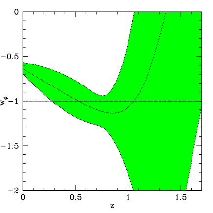
In fig. 6 we show the reconstructed equation of state factor $w_{\phi}$ for different values of $N$. The background cosmology is a cosmological constant model with $\Omega_{\rm m}=0.3$ and $\Omega_{\Lambda}=0.7$. In the top right panel we plot the mean values of the reconstructed $w_{\phi}$. We note that for $N=3$ fit (dotted line and top right panel) the mean value does not represent the theoretical $w_{\phi}$ well. This is because in order to reconstruct $w_{\phi}$ we need the second derivative of the coordinate distance $r(z)$ (eqn. 23). The coordinate distance is already reduced by one order in $z$ compared to the luminosity distance so the $N=3$ fit might not represent sufficiently the evolution in $r(z)$ to produce a second derivative in $r(z)$ which represents the theoretical value at least roughly. The $N=4$ (solid line) and $N=5$ (dashed line) fit however reproduce, at least in the relevant redshift range, the theoretical value of $w_{\phi}$ to a satisfactory level. The $N=5$ fit naturally reproduces the $w_{\phi}$ better then the $N=4$ fit, however the errorbars for the $N=5$ fit (lower right panel) are much larger then for the $N=4$ fit (lower left panel). A fourth order polynomial, therefore, yields the best reconstruction for $w_{\phi}$ with the SNAP type specifications from table I. We note, however, from the lower left panel in fig. 6 that for the 4th order polynomial fit we can only reproduce $w_{\phi}$ in the required range if $-1.3<w_{\phi}<-0.7$, at the $1\sigma$ level.

As we saw in the previous section it seems nearly impossible to make any predictions about the equation of state factor $w_{\phi}$ with the SNAP type specifications. However, the problem could be the polynomial fit and not the SNAP experiment. If we assume for example a constant $w_{\phi}$ and try to reconstruct it with a polynomial fit of the luminosity distance, we can show analytically that no finite order polynomial can do this exactly. Even in the extreme case of just a pure cosmological constant model with $\Omega_{\Lambda}=1$ or the SCDM model with $\Omega_{\rm m}=1$ the polynomial can not fit it exactly. This problem was recognized in [46] and they suggested to use Padé approximants or even splines. In [47] a rational function is used which at least allows that the extreme cases of $\Omega_{\Lambda}=1$ and $\Omega_{\rm m}=1$ to be fitted with an exact relation. This method has been improved due to the introduction of a more complicated rational function with more free parameters [85]. A problem with all these reconstruction methods is that we need, the matter density $\Omega_{\rm m}$ as another input parameter as seen in eqn. (23). A further problem is that in order to reconstruct $w_{\phi}$ we have to calculate second order derivatives in $r(z)$ which will in general, increase the errorbars on the reconstructed equation of state factor. We propose a fit which has been discussed recently [86, 87, 88] allowing one to read off the equation of state factor directly with no reconstruction as in eqn. (23) and also includes the possibility to fit for $\Omega_{\rm m}$ in a more natural way.

We expand the equation of state factor into its redshift evolution

$$w_{\phi}=\sum_{i=0}^{N}w_{i}\left(1+z\right)^{i}\,,$$ (25)

where we chose the expansion in $(1+z)$ for computational convenience. With this expansion and eqns. (2),(22) we obtain the luminosity distance in a flat universe

$$d_{\rm L}^{\rm fit}(z)=\frac{c(1+z)}{H_{0}}\int\limits_{0}^{z}\frac{\left(1+z^{\prime}\right)^{-3/2}}{\sqrt{\Omega_{\rm m}+\Omega_{\phi}\left(1+z^{\prime}\right)^{3w_{0}}\exp\left\{3\sum\limits_{i=1}^{N}\frac{w_{i}}{i}\left[\left(1+z^{\prime}\right)^{i}-1\right]\right\}}}\,dz^{\prime}\,,$$ (26)

with $\Omega_{\phi}=1-\Omega_{\rm m}$. We note that for $w_{i}=0$ for $i\geq 1$ and $w_{0}=-1$ we obtain the standard result for the cosmological constant. In the following discussion we take $\Omega_{\rm m}=0.3$ fixed and later we examine the fit with different prior information on $\Omega_{\rm m}$.

The fit is done by minimizing the $\chi^{2}$ function

$$\chi^{2}\left(\left\{w_{i}\right\}\right)=\sum_{k=0}^{N_{z}}\left[\frac{d_{\rm L}(z_{k})-d_{\rm L}^{\rm fit}(z_{k})}{\delta d_{\rm L}(z_{k})}\right]^{2}\,,$$ (27)

with $\delta d_{\rm L}(z_{k})=\sigma_{\rm mag}d_{\rm L}(z_{k})\ln(10/5)$, the uncertainties in $d_{\rm L}(z)$ as the weight on the particular data points. The sum runs over the whole redshift range from table I, with $N_{z}$ the overall number of measurement redshifts. Again we assume that the redshift range is split into equidistant samples in the four ranges from table I. We minimize this rather complicated expression with the MINUIT routine from the CERN program library which also delivers the covariance matrix on the parameters.

FIG. 7.: The fit from eqn. (26) for the periodic potential as the cosmological background. We plot the fitted $d_{\rm L}^{\rm fit}$ with respect to the theoretical luminosity distance $d_{\rm L}$ in percent (%). The dotted line is the $N=0$ fit, the solid line the $N=1$ fit and the dashed line the $N=2$ fit. The left panel is the one with $\Omega_{\rm m}=0.3$ as a prior and the right one has just the constraint that $0\leq\Omega_{\rm m}\leq 1$.

In fig. 7 we plot the fit for different values of $N$ for the periodic potential as the dark energy model. We choose this model because we see in fig. 5 that the equation of state factor for this model is evolving within the relevant range. For a cosmological constant model a fit with $N=0$ should be the best, because it is exact and we do not gain any information by going to higher order. In fig. 7 we note that the $N=0$ fit, with $\chi^{2}\approx 31$, is a relatively poor fit of the theoretical values if we set a prior of $\Omega_{\rm m}=0.3$ (left panel). The first order results in a satisfactory fit with $\chi^{2}\approx 0.47$ and $N=2$ improves this result only slightly, with $\chi^{2}=7.3\times 10^{-3}$. So in order to study the luminosity distance $d_{\rm L}$ the first order fit seems to be sufficient. If we release the prior on $\Omega_{\rm m}$ and just constrain the matter contents of the universe by $0\leq\Omega_{\rm m}\leq 1$ the $N=1$ and $N=2$ fit are indistinguishable and fit reasonably well. It appears that the $w_{\phi}$ fit (eqn. 26) leads to more accurate results than the polynomial fit (eqn. 21) with less free parameters!

FIG. 8.: Relative accuracy of the rational fit (dotted line), the quadratic and cubic polynomial fit (dashed line) and the linear and quadratic $w$-expansion (solid line). The cosmology is taken from the periodic potential.

In fig. 8 we plot the relative accuracy of the different fits, for an unweighted sampling points. We recognize that the cubic polynomial- and quadratic $w$-expansion lead to the best fit. This results holds also if we use the weights from the SNAP specifications. We performed this comparison for the SUGRA and the periodic potential models as well as for a toy model [88]. For the cosmological constant the $w$-expansion results by construction to the best results because the fit is “exact”. We expect that this behaviour holds as well for the nearly constant models, like the two exponentials model.

FIG. 9.: The relative magnitude plots for the $N=0$ fit in the left panel and the $N=1$ fit in the right panel. The light grey lines are the theoretical values and the dark lines are the fitted results. The line styles are the same as in fig. 5.

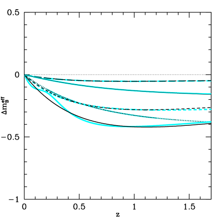
In fig. 9 we plot the results of the constant, $N=0$, fit and the linear, $N=1$, fit for a few of the sample of dark energy models which we have discussed (black lines) and their theoretical values (grey lines). We note that for the models which do not evolve much such as the inverse tracker (dotted line) and the pure exponential (long dashed line), the constant fit seems to be sufficient. However, for the SUGRA model (thin solid line) and the periodic potential (short dashed line) only the first order fit is acceptable. Note that both orders are not a good enough to fit the PNGB model (thick solid line).

In the following we will discuss the resulting $w_{\phi}(z)$ from the fit. First, we have to know the error matrix which is calculated as the inverse of the second derivative of the $\chi^{2}$-function at its minimum

$$\sigma_{ij}^{-1}=\left.\frac{\partial^{2}\chi^{2}\left(\left\{w_{i}\right\}\right)}{\partial w_{i}\partial w_{j}}\right|_{\left\{w_{i,j}=w_{i,j}^{\rm min}\right\}}\,,$$ (28)

which is a valid approximation if the $\chi^{2}$ function has an approximately parabolic shape around its minimum. MINUIT also calculates the marginalized errors on the parameters by calculating the values of the parameters for $\chi^{2}_{\rm min}+\Delta\chi^{2}$ with $\Delta\chi^{2}=1$. We used both methods and found that they give consistent results. The errors on $w_{\phi}$ are then given by Gaussian error propagation

$$\delta w_{\phi}^{2}=\sum_{ij}\frac{\partial w_{\phi}}{\partial w_{i}}\frac{\partial w_{\phi}}{\partial w_{j}}\sigma_{ij}=\sum_{ij}\left(1+z\right)^{i+j}\sigma_{ij}\,.$$ (29)

FIG. 10.: The equation of state factor $w_{\phi}$ for the periodic model. The theoretical value is $w_{\phi}(z)$ is given by the thin dotted line. In the top left panel we plot the mean values for the fitted $w_{\phi}$ with the dotted line for the $N=0$ fit, the solid line for the $N=1$ and the dashed line the for $N=2$ fit. The top right panel is the $N=0$ fit with the shaded region representing the $1\sigma$ uncertainty levels. The lower left panel is the same plot for $N=1$ and the lower right panel for $N=2$.

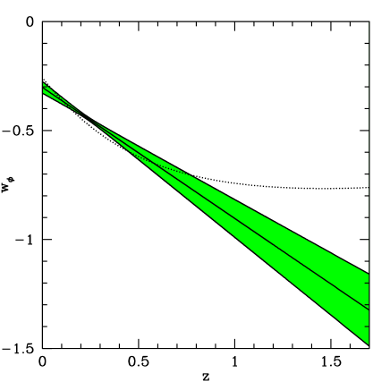
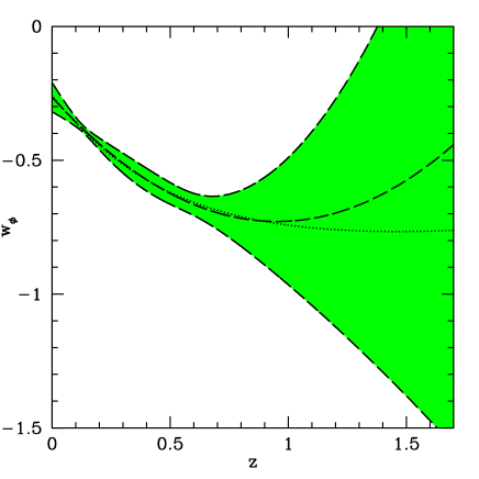
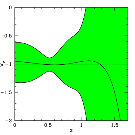
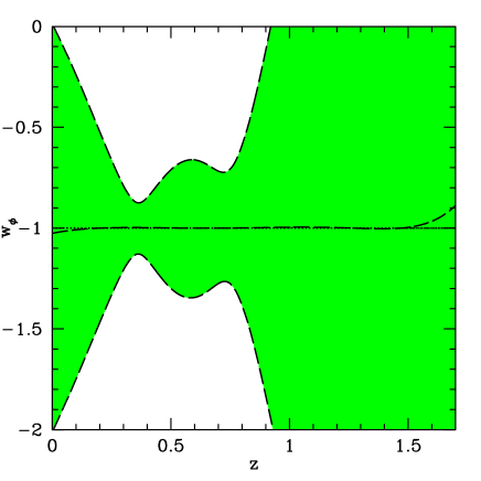
In fig. 10 we plot the resulting $w_{\phi}$ for different orders $N$ of the fit in eqn. (26) with the periodic potential as background cosmology. In the top left panel we plot the mean values and the theoretical curve (thin dotted line). The dashed line is for the $N=0$ fit and we recognize that a $w_{\phi}=w_{0}=const.$ fit can not reproduce the evolving model. The $N=1$ fit (solid line) already represents some evolution, so for $z>0.6$ the fit becomes fairly poor. The dashed line is the quadratic, $N=2$, fit, which leads to a better result than the linear fit. In the top right panel we show the constant, $N=0$ fit with it’s very small errorbars, in the lower left panel the $N=1$ fit and in the lower right panel the $N=2$ fit with the errorbars. We recognize that the errorbars for the $N=1$ and $N=2$ fit are roughly on the same level for $z<0.7$, but then the errorbars of the $N=2$ fit increase rapidly. In general the errorbars on the $N=1$ fit are smaller then the ones on the $N=2$ fit, since there are less degrees of freedom.

FIG. 11.: The fitted $w_{\phi}$ for different dark energy models. The solid lines and the dark shaded region corresponds to the mean and $1\sigma$ error regions of the pure cosmological constant model. The dashed lines and the light shaded region to the periodic potential (top left panel), the inverse tracker potential (top right panel) and the SUGRA potential (lower left panel). In the lower right panel we show the theoretical (dotted line) and reconstructed (solid line) $w_{\phi}$ of the PNGB model.

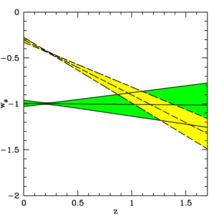
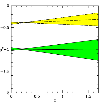
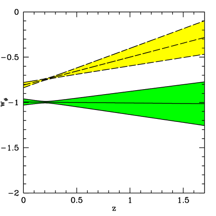
In fig. 11 we plot the periodic potential model (top left panel), the inverse tracker (top right panel) and the SUGRA inspired dark energy model (bottom left panel). The light shaded regions are the $1\sigma$ confidence levels. In each plot we show the cosmological constant model for comparison (dark shaded region). We recognize that for the fit from eqn. (26) we can distinguish the $w_{\phi}(z)$ evolution from a cosmological constant on the $1\sigma$ level. We also performed the fits for the $N=2$ approximation and got still better results as for the polynomial fit, despite the increased size of the errorbars. In the lower right panel we show the mean of the fit for the PNGB model (solid line). We recognize that the $w_{\phi}$ fit is not appropriate for the oscillating PNGB model (dotted line). This behavior does not improve much if we apply a second order fit. The polynomial fit hardly can distinguish the reconstructed $w_{\phi}$ of the inverse tracker, the periodic and the SUGRA potential from a cosmological constant, although their theoretical $w_{\phi}$ is completely different from $w_{\phi}=-1$ as evident from fig. 5.

We will now examine the question of whether we can reconstruct an evolving $w_{\phi}$ with the SNe observations. Since the $\chi^{2}$ values for the $N=1$ fit where sufficient and the errorbars on this fit are relatively small we will concentrate in the following on this linear fit. In order to be able to decide if a model is evolving we perform a change of variable to more convenient expansion. We can rewrite eqn. (25) as

$$w_{\phi}(z)=\sum_{i=0}^{N}w_{i}\left(1+z\right)^{i}=\sum_{i=0}^{N}{\tilde{w}}_{i}z^{i}\,,$$ (30)

with

$${\tilde{w}}_{i}=\sum_{k=0}^{N}{k\choose i}w_{k}\,.$$ (31)

For the $N=1$ fit this leads to ${\tilde{w}}_{0}=w_{0}+w_{1}$ and ${\tilde{w}}_{1}=w_{1}$. The errors in the new expansion coefficients ${\tilde{w}}_{i}$ can, again, be found by Gaussian error propagation

$$\delta{\tilde{w}}_{i}^{2}=\sum_{kl}{k\choose i}{l\choose i}\sigma_{kl}\,.$$ (32)

We calculated these expansion coefficients and their $1\sigma$ errors for all the models.

	${\tilde{w}}_{0}$	$\delta{\tilde{w}}_{0}$	${\tilde{w}}_{1}$	$\delta{\tilde{w}}_{1}$	theoretical evolution	evolution reconstructed
$\Lambda$	$-1.00$	$0.035$	$-0.011$	$0.16$	$-$	$-$
trapped minimum	$-0.99$	$0.035$	$-0.0057$	$0.16$	$-$	$-$
Brane	$-0.97$	$0.034$	$0.028$	$0.16$	$+$	$-$
two exp.	$-0.95$	$0.034$	$-0.016$	$0.16$	$-$	$-$
periodic	$-0.30$	$0.027$	$-0.60$	$0.11$	$+$	$+$
pure exp.	$-0.84$	$0.033$	$-0.14$	$0.15$	$0$	$0$
PNGB	$-0.00$	$0.025$	$-0.94$	$0.10$	$+$	$+$
SUGRA	$-0.81$	$0.029$	$0.31$	$0.13$	$+$	$+$
exp. tracker	$-1.00$	$0.035$	$-0.011$	$0.16$	$-$	$-$
inv. tracker	$-0.40$	$0.025$	$0.054$	$0.10$	$-$	$-$

TABLE II.: The evolution coefficients with errorbars for the linear fit $w_{\phi}={\tilde{w}}_{0}+{\tilde{w}}_{1}z$. “$+$” denotes evolution, “$-$” no evolution and “$0$” marginal evolution.

In table II we present the expansion coefficients for the dark energy models we have discussed. We note that we obtain evidence at the $1\sigma$ level for evolution for the SUGRA and periodic potential. The only model which is not reproduced correctly in the context of an evolving $w_{\phi}$ is the brane-inspired model. This is because equation of state factor for the brane model changes only relatively early ($z>0.8$), where the data does not have so much weight. Note although we get a consistent result for the PNGB model, the fit of $w_{\phi}$ is relatively bad (fig. 11, lower right panel) and it has with $\chi^{2}\approx 24.8$ an unacceptable luminosity distance fit. We also note in fig. 11 that the inverse tracker model is not only evolving, but also does not behave like a cosmological constant, since $w_{\phi}\approx-0.4$, which is consistent with the result in table II.

FIG. 12.: The joint confidence regions in the ${\tilde{w}}_{0}-{\tilde{w}}_{1}$ plane. In the left panel we show the $68.3\%$ confidence regions and in the right panel the $99\%$ region. The shaded region is the uncertainty region for an arbitrary but constant equation of state factor with $-1<w_{\phi}<0$. The thin short dash ellipse is for the trapped minimum models, the thin dot - short dash ellipse is for the brane inspired potential, the thin short dash - long dash ellipse for the potential which involves two exponentials, the thick short dashed ellipse for the periodic potential, the thick long dashed ellipse for the pure exponential, the thin solid ellipse for the Supergravity inspired potential, the thin long dashed ellipse for the exponential tracker solution, and the thick dotted ellipse for the inverse tracker.

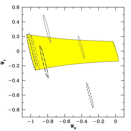
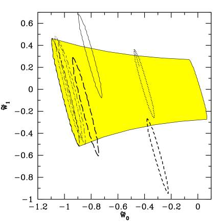
In fig. 12 we show the joint probability contours in the ${\tilde{w}}_{0}-{\tilde{w}}_{1}$ plane, for the $68.3\%$ and $99\%$ confidence levels. The confidence levels for the joint probability are calculated as the regions with $\chi^{2}=\chi^{2}_{\rm min}+\Delta\chi^{2}$ with $\Delta\chi^{2}=2.3$ and $\Delta\chi^{2}=9.21$ respectively, which is valid since the errors are symmetric. The shaded region is the $68.3\%$, resp. $99\%$, confidence region for $-1<w_{\phi}=const<0$. In this plot we see that only the SUGRA (thin solid ellipse) and periodic potential (thick short dashed ellipse) can be distinguished from a constant $w_{\phi}$ at the $1\sigma$ level (left panel). At the $99\%$ level (right panel ) it is even harder to extract evolving models and only the periodic potential can be distinguished from $w_{\phi}=const$. However, if we are just interested in whether a model is evolving we have to concentrate on the parameter ${\tilde{w}}_{1}$ and marginalize over ${\tilde{w}}_{0}$, which corresponds to the projection of the confidence region with $\Delta\chi^{2}=1$ for the $1\sigma$ errorbars[89, 90]. But even if we consider the marginalized errors on ${\tilde{w}}_{1}$ in table II the only model for which we can find evidence for evolution with $99\%$ confidence is the periodic potential. Note that we have omitted the PNGB model in this discussion because the reproduced $w_{\phi}$ for this model is not valid.

Up to now we have used a fixed prior on $\Omega_{m}$ to fit the luminosity distance and reconstruct the equation of state factor $w_{\phi}$. We will now discuss how our results will change if we have no prior information on $\Omega_{\rm m}$ and use just the constraint $0\leq\Omega_{\rm m}\leq 1$.

	$w_{0}$	$\delta w_{0}$	$w_{1}={\tilde{w}}_{1}$	$\delta w_{1}=\delta{\tilde{w}}_{1}$	$\Omega_{\rm m}$	$\delta\Omega_{\rm m}$
$\Lambda$	$-0.94$	${}_{-0.46}^{+1.08}$	$-0.063$	${}_{-1.10}^{+0.64}$	$0.31$	${}_{-0.31}^{+0.07}$
inv. tracker	$-0.44$	${}_{-0.15}^{+1.53}$	$-0.01$	${}_{-0.99}^{+0.99}$	$0.38$	${}_{-0.38}^{+0.23}$
periodic	$0.75$	${}_{-0.65}^{+0.86}$	$-1.10$	${}_{-0.83}^{+0.69}$	$0.41$	${}_{-0.21}^{+0.08}$
SUGRA	$-1.10$	${}_{-0.20}^{+1.31}$	$0.21$	${}_{-1.42}^{+0.29}$	$0.34$	${}_{-0.34}^{+0.13}$

TABLE III.: The expansion parameters from eqn. (25) for a $N=1$ fit, where $\Omega_{\rm m}$ is only constrained by $0\leq\Omega_{\rm m}\leq 1$. The underlying theoretical models have all $\Omega_{\rm m}=0.3$.

In table III we show the results of the fit with $N=1$ and no prior on $\Omega_{\rm m}$. Note that we show the quantities $w_{i}$ and not ${\tilde{w}}_{i}$. The reason for this is, that if we include $\Omega_{\rm m}$ as parameter to fit, the errors on the fitted $w_{i}$ are not symmetric, and therefore not Gaussian. Therefore, we can not perform the error propagation using eqn. (32). We study two models which are theoretically not evolving, $\Lambda$ and the inverse tracker, and two models which have an evolving $w_{\phi}$, the periodic and SUGRA potential. First, we note that the errorbars on the fitted value of $\Omega_{\rm m}$ are large, and that the mean value, in the case of the periodic and inverse tracker potential is displaced from the theoretical value by over $25\%$! Although, due to the large errorbars the mean value and the theoretical value always lie within the $1\sigma$ errorbars. In the case of the periodic potential we can recover evolution marginally, since ${\tilde{w}}_{1}=-1.10^{+0.69}_{-0.83}$. However, at the $99\%$ level we can not gain any evidence for evolution. For the SUGRA model we can not reconstruct evolution since the obtained value for ${\tilde{w}}_{1}$ is consistent with no evolution (${\tilde{w}}_{1}=0$) already on the $1\sigma$ level. We conclude, therefore, that if we fit simultaneously for $\Omega_{\rm m}$ and $w_{1}$ simultaneously it is poor and has large errorbars.

	$w_{0}$	$\delta w_{0}$	$\Omega_{\rm m}$	$\delta\Omega_{\rm m}$
$\Lambda$	$-0.99$	$0.06$	$0.30$	$0.02$
inv. tracker	$-0.45$	$0.11$	$0.37$	$0.12$
periodic	$-0.28$	$0.01$	$0.00$ (!)	$0.03$
SUGRA	$-0.91$	$0.07$	$0.38$	$0.03$

TABLE IV.: The fit results for $\Omega_{\rm m}$ and $w_{0}$ using the $N=0$ fit.

In table IV we show the results for the constant $N=0$ fit. First, we note that the errorbars on $w_{0}$ and $\Omega_{\rm m}$ are much smaller than for the linear $N=1$ fit. However, we do not expect that this will work for models which are evolving. In fact, we recognize that for the periodic potential we get $\Omega_{\rm m}=0$ where this is only the “best fit” value because of the constraint on $\Omega_{\rm m}$. If we release the constraint for this fit, $\Omega_{\rm m}$ floats to negative and non-physical values. This is because the periodic potential has an evolving $w_{\phi}$ and an $N=0$ fit can not reproduce such an evolving model. The pure $\Lambda$, the SUGRA and the inverse tracker model seem to give reasonable results, apart from the SUGRA model results in a too large value for $\Omega_{\rm m}$, where the true value of $\Omega_{\rm m}$ is outside the $1\sigma$ errorbar. This is again due to the fact that $w_{\phi}$ is evolving for the SUGRA model.

FIG. 13.: The joint probabilities for $\Omega_{\rm m}$ and $w_{0}$ for the $N=0$ fit for the $\Lambda$ model (solid line) and the SUGRA model (dotted line). The dark shaded region is the $68.3\%$ confidence level and the brighter shaded region the $99\%$ level.

In fig. 13 we show the joint probability contours in the $w_{0}-\Omega_{\rm m}$ plane. The solid line is the pure cosmological constant and the dotted line the SUGRA model. We note that even for a marginally evolving model like the SUGRA model that the $N=0$ fit gives a reasonable result. Note that we did not impose a constraint of $w_{0}\geq-1$ for the $N=0$ fit. This constraint basically results in a cut off of the confidence regions in fig. 13 below the $w_{0}=-1$ line. To conclude we remark that we either need a fixed prior on $\Omega_{\rm m}$ to be able to tell whether the equation of state factor $w_{\phi}$ is evolving, or we only consider the constant contribution to $w_{\phi}$ which would allow us to establish both $\Omega_{\rm m}$ and $w_{\phi}$ accurately. In section VI we will now investigate how different satellite designs and priors on $\Omega_{\rm m}$ may change this behavior.

VI Impact of experiment design parameters and priors on the matter content

We will now discuss the impact of the specific SNAP setup on the estimation on $w_{\phi}$.

FIG. 14.: The dependence of the statistical errors $\sigma_{ij}$ on the SNAP specifications for the linear, $N=1$, fit. The dotted line is $\sigma_{00}=\delta w_{0}^{2}$ the dashed line is $-\sigma_{01}=\left<\delta w_{0}\delta w_{1}\right>$ and $\sigma_{11}=\delta w_{1}^{2}$ the solid line. In the top left panel we show the dependence on the number of observed redshifts $N_{z}$ where the maximal redshift is fixed to $z_{\rm max}=2$ and the statistical error on the magnitude is $\sigma_{\rm mag}=0.15\,{\rm mag}$. In the top right panel we show the dependence on $\sigma_{\rm mag}$, where the number of redshifts is fixed to be $N_{z}=2000$. In the lower left panel we plot the error matrix as a function of the maximal observed redshift, where we fix the number of observed SNe to $2000$ and $\sigma_{\rm mag}=0.15\,{\rm mag}$. In the lower right panel we show the evolution of the statistical error with the maximal observed redshift assuming that $90\%$ of the observations are in the low redshift region $0<z<1.2$.

In fig. 14 we show the dependence of the error matrix $\sigma_{ij}$ on the experimental parameters using the $N=1$ fit for the periodic potential model with $\Omega_{\rm m}=0.3$ fixed. The dotted line is $\sigma_{00}$, the dashed line $-\sigma_{01}$ and the solid line is $\sigma_{11}$. In the top left panel we show the dependence on the observed number of redshifts $N_{z}$ where we keep the magnitude error fixed at $\sigma_{\rm mag}=0.15\,{\rm mag}$ and the maximal observed redshift is $z_{\rm max}=2$. We recognize that the variances scale as expected with $1/N_{z}$, or the errors with $1/\sqrt{N_{z}}$. In the top right panel we show that the dependence on the absolute magnitude error $\sigma_{\rm mag}$, where the maximal redshift is fixed to $z_{\rm max}=2$ and the number of observed SNe is $N_{z}=2000$. We note that the error matrix is increasing as $\sigma_{\rm mag}$ increases as expected. The conservative limit on the total dispersion is $\sigma_{\rm mag}=0.15\,{\rm mag}$ as stated in table I, which includes using the best currently known methods of standardizing and calibrating the luminosity of type Ia SNe with a residual dispersion of $0.12\,{\rm mag}$ and a measurement uncertainty of $0.09\,{\rm mag}$ after correcting for extinction and using the color of the SNe. Optimistically view that with new methods and all the additional information which is available for the SNe with SNAP might reduce the residual dispersion from the standardization and calibration to $0.05\,{\rm mag}$, although we do not expect to the improvement in the measurement uncertainties to be more then $0.08\,{\rm mag}$. Therefore, the most optimistic choice results in $\sigma_{\rm mag}=0.09\,{\rm mag}$. We see in the top right panel of fig. 14 that if we improve the statistical error from $\sigma_{\rm mag}=0.15\,{\rm mag}$ to $\sigma_{\rm mag}=0.09\,{\rm mag}$ the uncertainties on the fit parameters $w_{i}$ improve by $70\%$. This means we are able to reconstruct evolution even for the marginally evolving pure exponential model (thick long dashed line, fig. 5) at the $68.3\%$ level with ${\tilde{w}}_{1}=-0.14$ and $\delta{\tilde{w}}_{1}=0.09$.

In the lower left panel of fig. 14 we plot the dependence on the maximal observed redshift where we keep the number of observed SNe redshifts fixed to $2000$ and $\sigma_{\rm mag}=0.15\,{\rm mag}$. It is evident from the plot that we can gain most accuracy if the observations are done up to a redshift of $z_{\rm max}\approx 3$. Beyond this redshift there is no further improvement. In the lower right panel we show more realistic result of increasing the maximal observed redshift on the statistical error. In this plot we assume that there is a fixed threshold number $\Delta n$ of photons which have to arrive in the detector in order to observe an SNe. We neglect the effects of color in this analysis. The brightness or flux of a SNe is ${\cal F}={\cal L}/4\pi d_{\rm L}^{2}$ and the measured flux in the detector is ${\cal F}\propto(\Delta n)/(\Delta A\Delta t)$, where $\Delta A$ is the effective area of the detector. From this relation we can work out the time $\Delta t$ for which we have to measure the flux from a SNe at a particular redshift in order to observe it. We assume that for a fraction $p$ of the total observation time $T$ we find SNe in a low redshift region $0<z<z_{l}$ and a fraction $(1-p)$ in the high redshift region $z_{l}<z<z_{\rm max}$. In order to calibrate the relation we fix the low redshift region with $z_{l}=1.2$ and the number of observed SNe in this region to ${\cal N}_{l}=1850$ as in table I. The number of observed SNe in the high redshift region is then approximately

$${\cal N}_{h}\approx{\cal N}_{l}\frac{1-p}{p}\frac{\left(1+z_{l}+z_{l}^{2}/3\right)}{\left(1+z_{l}\right)^{2}+\left(1+z_{l}\right)\left(z_{\rm max}-z_{l}\right)+\left(z_{\rm max}-z_{l}\right)^{2}/3}\,.$$ (33)

In the lower right panel of fig. 14 we assume that for $p$ equivalent to 90% of the total observation time we discover SNe in the low redshift region $0<z<1.2$. If we choose $z_{\rm max}=1.7$ we observe ${\cal N}_{h}=65$ SNe in the region $1.2<z<1.7$ in agreement with the values given in table I. For redshifts $z\leq 1.2$ a similar equation to eqn. (33) holds, where in this case the entire observation time is spent in the low redshift region. If we observe out to a redshift of $z_{\rm max}=2.5$ we can observe ${\cal N}_{h}=48$ SNe. From fig. 14 we recognize that if we go from $z_{\rm max}=1.7$ to $z_{\rm max}=2.5$ we improve the statistical error by $10\%$. We see from table II that such an improvement of the statistical error on ${\tilde{w}}_{1}$ is only marginal and we can not distinguish more models or establish evolution for more models when compared to the case when we can just measure out to redshifts of $z_{\rm max}=1.7$.

We notice in fig. 11, that the “reconstructed” $w_{\phi}$ has a region where the errorbars are relatively small, which is for the $N=1$ fit in eqn.(26) around $z_{f}\approx 0.2$. We find the position $z_{f}$ of the feature by minimizing $\delta w_{\phi}$ in eqn.(29) assuming a symmetric error matrix and a linear fit

$$1+z_{f}=-\frac{\sigma_{01}}{\sigma_{11}}\,,$$ (34)

with $\sigma_{ij}$ the covariance matrix from eqn.(28). This feature corresponds to the “sweet spot” in [91] and is also the redshift around which [91] perform the $w$-expansion in order to obtain uncorrelated expansion coefficients. From this expression we already expect that the position of the feature will not vary if we change the number of data points $N$ or the statistical error on the magnitude $\sigma_{\rm mag}$ and this behavior was established by numerical experiments.

FIG. 15.: The shift of the minimal error region $z_{f}$ with the change of the maximal observed redshift $z_{\rm max}$.

In fig. 15 we plot the dependence of the position of the feature $z_{f}$ versus the maximally measured redshift for the periodic potential. We plotted the behavior up to the very high redshift $z=20$ and recognize that even for such high redshifts the feature is still below $z_{f}=0.7$. The transition from matter to vacuum domination (when the energy density of the dark energy field dominates over the one of matter) for the periodic model is around $z\approx 0.75$. So even if one could measure SNe at the unrealistic distance of $z=20$ we still do not have the smallest errorbars in the interesting $z=0.75$ region. This behavior is similar for all the dark energy models we studied.

We examine now the behavior of the statistical error if we fit for the parameters $w_{0}$ and $\Omega_{\rm m}$.

FIG. 16.: Improvement of the statistical error on $w_{0}$ and $\Omega_{\rm m}$ for the fitted $\Lambda$ model. The solid line is $\sigma_{11}=\delta\Omega_{m}^{2}$, the dashed line is $-\sigma_{01}=\left<\delta w_{0}\delta\Omega_{m}\right>$ and the dotted line is $\sigma_{00}=\delta w_{0}^{2}$. In the left panel we show the improvement of the uncertainty on the fit parameters due to increasing the maximal observed redshift, where we assume that for $90\%$ of the observation time we find low redshift SNe. In the right panel we show the dependence of the statistical error on the residual magnitude dispersion.

In fig. 16 we show the behavior of the covariance matrix $\sigma_{ij}$ with a varying $z_{\rm max}$ and $\sigma_{\rm mag}$. In this case $\sigma_{11}$ is the square of the error on the best fit $\Omega_{\rm m}$. In the left panel we show the evolution with the maximal measured redshift where we construct the sampling rate in the high and low redshift bins with eqn. (33) and ${\cal N}_{l}=1850$, $z_{l}=1.2$. We recognize that we improve the statistical uncertainty by $14\%$ if we measure SNe out to redshifts of $z_{\rm max}=2.5$ instead of $z_{\rm max}=1.7$. In the right panel we change the residual dispersion $\sigma_{\rm mag}$ with the rest of the parameters fixed to the SNAP specification in table I. The improvement on the statistical error by going from $\sigma_{\rm mag}=0.15\,{\rm mag}$ to $\sigma_{\rm mag}=0.09\,{\rm mag}$ is $64\%$. We will discuss the relevance of this improvement when we examine different priors on the fit parameters $w_{0}$, $w_{1}$ and $\Omega_{\rm m}$. However we conclude that an improvement of the measurement uncertainties is far more relevant than the ability to observe SNe at larger redshifts.

We will now discuss how different priors on the fit parameter $\Omega_{\rm m}$ influence the accuracy. We have discussed just the most extreme cases of priors on the $N=1$ fit with either $\Omega_{\rm m}=0.3$ fixed or $w_{1}=0$ fixed.

FIG. 17.: Error contours of the SUGRA model with different priors on $\Omega_{\rm m}$ in the ${\tilde{w}}_{0}$–$w_{1}$ plane. The solid line contours are the $39.3\%$ joint probability regions, which project to $1\sigma$ errors on the axis and shaded regions represent the $68\%$ or $1\sigma$ joint probabilities. The range of increasingly larger contours represents the result using prior knowledge on $\Omega_{m}$ with increasingly poorer uncertainty, $\sigma_{\Omega_{m}}=\delta\Omega_{\rm m}$. The unlabelled, black dotted curve corresponds to the projected-1$\sigma$ error contour obtained for more optimistic dataset specifications and with a prior of $0.25\leq\Omega_{m}\leq 0.35$.

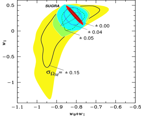
In fig. 17 we show the decreasing errorbars in the ${\tilde{w}}_{0}-w_{1}$ plane with different Gaussian priors on $\Omega_{\rm m}$. Note that we analyzed the full likelihood function and did not assume a Gaussian shape for the probability distribution. The current observations provide either just a crude measurement or upper limits on $\Omega_{\rm m}$. From [59] we obtain $\Omega_{\rm m}=0.2^{+0.3}_{-0.1}$ which is too crude to result in a significant improvement on our $w_{0}$-$w_{1}$-$\Omega_{\rm m}$ estimation. The X-ray observation in [21] give an upper limit of $\Omega_{\rm m}\leq 0.32\pm 0.01$ and the Sunyaev Zel’dovich results in [60] are $\Omega_{\rm m}\leq 0.34^{+0.05}_{-0.03}$. Future Sunyaev Zel’dovich surveys [60, 92] can possibly determine $\Omega_{\rm m}$ up to an accuracy of $3\%$ if one considers in conjunction with CMB measurements[93]. Future X-ray surveys could determine $\Omega_{\rm m}$ to even higher accuracy independent of any other measurement[93].

We observe in fig. 17 that only very tight bounds of $\Omega_{\rm m}\pm\delta\Omega_{\rm m}$ with $\delta\Omega_{\rm m}\leq 0.05$ improve the statistical errorbars which are stated in table III. If we improve the statistical error on the magnitude to $\sigma_{\rm mag}=0.09$ and double the number observed SNe we can even further improve the accuracy (dotted line in fig. 17).

prior $\delta_{\Omega_{m}}$	measurement $\sigma_{\rm mag}$	$\delta_{w_{0}}$	$\delta_{w_{1}}$
No ${\Omega_{m}}$ prior; $w_{1}=0$	0.15	0.06
0.15	0.15	0.15	0.6
0.05	0.15	0.06	0.2
”	0.09	0.05	0.12
0.04	0.15	0.05	0.16
0     (fixed ${\Omega_{m}}$)	0.15	0.03	0.12

TABLE V.: Statistical measurement uncertainties on $w_{0}$ and $w_{1}$, given supernova magnitude measurement uncertainty, $\sigma_{\rm mag}$, and a range of uncertainties, $\delta_{\Omega_{m}}$, in the independent prior knowledge of $\Omega_{m}$. (As in fig. 17 , the Supergravity model is used here as the example, but the other models give comparable results.)

In table V we summarize our findings for the accuracy of the SNAP measurement with different priors on $\Omega_{\rm m}$. If we combine these findings with the results in table II we see that for the periodic potential the current accuracy on $\Omega_{\rm m}$ is sufficient to establish evolution at least on the $1\sigma$ level, however for the SUGRA model we need at least the tight prior with $\delta\Omega_{\rm m}=\pm 0.05$.

A further restrictive prior for the linear fit is $-1\leq w_{\phi}(z=0)<0$ which results in the constraint $-1<w_{0}+w_{1}<0$. The constraint $-1\leq w_{\phi}$ excludes non-minimally coupled scalar-tensor theories [76, 94, 95], which we have not included in our discussion. If we analyze the results for the $N=1$ fit with fixed $\Omega_{\rm m}$ this prior does not improve the statistical uncertainty. If we do not fix $\Omega_{\rm m}$, the constraint $-1<w_{0}+w_{1}<0$ for the linear fit, or $-1<w_{0}<0$ for the constant fit also does not improve the statistical errors. From this we conclude that either we use a tight measurement of $\Omega_{\rm m}$ from an independent observation or we can not establish evolution of $w_{\phi}$ for most of the dark energy models. A further prior we have used throughout this paper is the assumption that the universe is flat. For a non-flat universe the luminosity distance is given by

$$d_{\rm L}(z)=\frac{c\left(1+z\right)}{\sqrt{\left|\Omega_{k}\right|}H_{0}}{\cal S}\left(\sqrt{\left|\Omega_{k}\right|}\int\limits_{0}^{z}\left[\Omega_{k}(1+z^{\prime})^{2}+\Omega_{m}(1+z^{\prime})^{3}+\Omega_{\phi}(1+z^{\prime})^{3(w_{0}+1)}{\rm e}^{3w_{1}z^{\prime}}\right]^{-1/2}\;dz^{\prime}\right)\,,$$ (35)

with $\Omega_{k}=1-\Omega_{\phi}-\Omega_{m}$ and ${\cal S}(x)=\sin(x)$ for $\Omega_{k}<0$ and ${\cal S}(x)=\sinh(x)$ for $\Omega_{k}>0$.

FIG. 18.: The difference in magnitudes between non-flat models and the fiducial $\Lambda$ cosmology, where the ratio between $\Omega_{m}$ and $\Omega_{\phi}$ is fixed. The solid line is for $\Omega_{k}=-0.2$, the dotted line for $\Omega_{k}=0.2$, the short dashed line for $\Omega_{k}=-0.05$ and the long dashed line for $\Omega_{k}=0.05$. The data points correspond to the binned SNAP data as in fig.2.

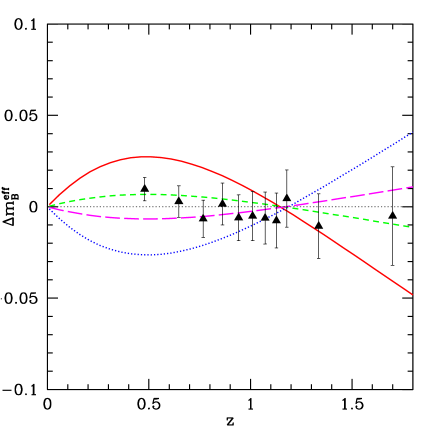
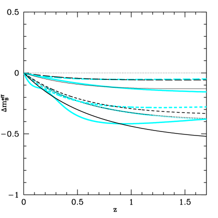
In fig.18 we show the magnitude difference to the fiducial $\Lambda$ model for models with non-vanishing curvature $\Omega_{k}$, where we fixed the ratio $\Omega_{m}/\Omega_{\phi}$. The solid line is for $\Omega_{k}=-0.2$ and the dotted line for $\Omega_{k}=0.2$. SNAP could clearly distinguish these models on the $1\sigma$ level. However the current uncertainties on the curvature from CMB and large scale structure observations are $\Delta\Omega_{k}=\pm 0.05$ on the $2\sigma$ level [15, 58]. The long and short dashed lines in fig.18 correspond to $\Omega_{k}=\pm 0.05$ and we see that with the SNAP data we can not improve the current constraints. The inclusion of a curvature term in the analysis presented in this paper in principle increases the uncertainty of the estimated parameters, however in the light that future CMB observations like MAP and Planck will provide even tighter constraints on the curvature (for Planck $\Delta\Omega_{k}=\pm 0.007$ [96]), we assume, as mentioned before, a fixed prior of $\Omega_{k}=0$.

We turn now to the question how systematic errors influence our ability to distinguish dark energy models and reconstruct the equation of state factor $w_{\phi}$. The systematic error in the luminosity distance is related to that in the magnitude $\sigma_{\rm sys}$ by

$$\pm\delta d_{\rm L}^{\rm sys}=\left(10^{\pm\frac{\sigma_{\rm sys}}{5}}-1\right)d_{\rm L}\,.$$ (36)

Since we marginalize over the magnitude zero point ${\cal M}$ in eqn.(5), we expect the systematic error for the magnitude to be zero for low redshifts. We assume a linear drift of the systematic error by

$$\sigma_{\rm sys}=\frac{{\hat{\sigma}_{\rm sys}}}{1.5}z\,,$$ (37)

where ${\hat{\sigma}_{\rm sys}}$ is the systematic error at a redshift of $z=1.5$.

FIG. 19.: The effects of the linear drifting systematic error on the fitted parameters. The dark shaded region corresponds to $68.3\%$ joint probability region of the models without systematic error, the light shaded regions to ${\hat{\sigma}_{\rm sys}}=\pm 0.02\,{\rm mag}$ and the transparent regions to ${\hat{\sigma}_{\rm sys}}=\pm 0.05\,{\rm mag}$. The ellipses with a solid margin are the results for the $\Lambda$ model. In the left panel we show the results for the $N=1$ fit with $\Omega_{\rm m}$ fixed. The dashed margins are from the periodic potential model. In the right panel the results for the $\Omega_{\rm m}$-$w_{0}$ fit are shown, where the dotted lines correspond to the SUGRA model.

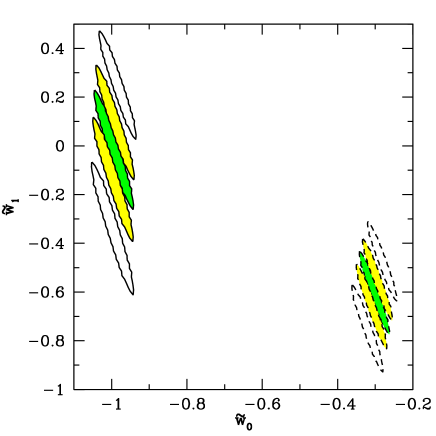
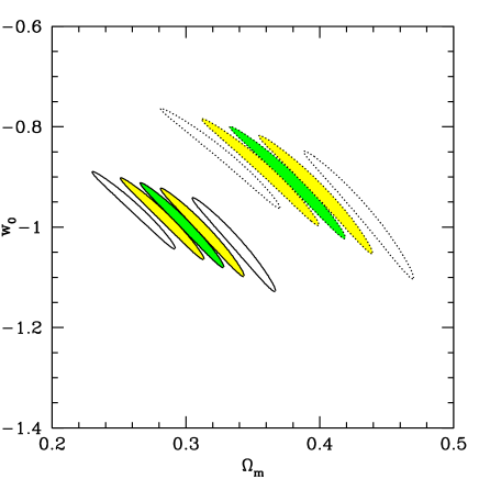
In fig. 19 we show the influences of the systematic uncertainty, where we plot the $68.3\%$ joint probability regions on the estimated parameters with the standard SNAP specifications from table I. The light shaded regions correspond to a systematic error of ${\hat{\sigma}_{\rm sys}}=\pm 0.02\,{\rm mag}$, the transparent regions to ${\hat{\sigma}_{\rm sys}}=\pm 0.05\,{\rm mag}$ and the dark shaded region is the result for no systematic error. In the left panel we show the result for the $N=1$ fit with a fixed $\Omega_{\rm m}$. We note that the linear drifting systematic error leads to a shift in the ${\tilde{w}}_{1}$ direction, but the marginalized error on ${\tilde{w}}_{0}$ changes only slightly. The shift for the periodic potential model (dashed lines) is much smaller than for the $\Lambda$ model (solid lines). But if we take into account the relative sizes of the statistical error depicted by the error ellipses, we find that the shift due the systematic error is roughly in agreement with these errors. In both cases the systematic error with ${\hat{\sigma}_{\rm sys}}=\pm 0.05\,{\rm mag}$ is only in marginal agreement with the reconstructed values of ${\tilde{w}}_{1}$ with no systematic error. The value of ${\tilde{w}}_{1}$ for the $\Lambda$ model is ${\tilde{w}}_{1}=-0.011$ and the one for the periodic potential is ${\tilde{w}}_{0}=-0.60$ if we do not include the systematic error. The $68.3\%$ joint probability regions for ${\hat{\sigma}_{\rm sys}}=\pm 0.05\,{\rm mag}$ only marginally overlap with these values in both cases. However, the $99\%$ confidence regions are all in agreement even in the shifted case with the theoretical mean values. We can reconstruct evolution of the periodic potential model even for ${\hat{\sigma}_{\rm sys}}=-0.05\,{\rm mag}$ which results in ${\tilde{w}}_{1}=-0.47$ and $\delta{\tilde{w}}_{1}=0.11$ which is still in agreement with ${\tilde{w}}_{1}\neq 0$ at the $3\sigma$ level. We also expect that we can distinguish the same models without inclusion of a systematic error since the main difference of the models is along the ${\tilde{w}}_{0}$ axis as evident from fig. 12. In the right panel we show the results for the $\Omega_{\rm m}$-$w_{0}$ fit, where the dotted ellipses correspond to the results from the SUGRA model. As before the estimate value of $w_{0}$ is not as strongly affected by the systematic error as the fitted value of $\Omega_{\rm m}$. Again the $68.3\%$ confidence levels for ${\hat{\sigma}_{\rm sys}}=\pm 0.05\,{\rm mag}$ (transparent regions) are only marginally in agreement with the fitted $\Omega_{\rm m}$ for no systematic error (dark shaded region). We conclude that the influence of the systematics is of significant importance for the estimated $\Omega_{\rm m}$ or ${\tilde{w}}_{1}$ only at the $1\sigma$ level, but is almost negligible for the estimation of the constant contribution ${\tilde{w}}_{0}$ to the equation of state factor $w_{\phi}$. In order to answer the question as to whether we can reconstruct evolution and $\Omega_{\rm m}$ of the periodic model with the SNAP experiment we have to take into account systematic errors. First, we realize that for the standard SNAP configuration from table I with a systematic error of ${\hat{\sigma}_{\rm sys}}=0.02$ and a statistical uncertainty we get for the best fit parameter, $w_{0}=0.75^{+0.86}_{-0.65}\pm 0.04$, $w_{1}=-1.07^{+0.69}_{-0.83}\pm 0.04$ and $\Omega_{\rm m}=0.41^{+0.08}_{-0.21}{}^{+0.02}_{-0.03}$, where the second error is due to the systematics. We recognize that we can only reconstruct evolution, which is the inconsistency of $w_{1}$ with a zero mean, at the $1\sigma$ level and that the statistical error on $\Omega_{\rm m}$ is nearly of the order of the mean ($50\%$). The limited amount of linear evolution we can reconstruct at the $3\sigma$ level with this experimental setup is $w_{1}\approx\pm 2.4$ and none of the models we studied has such a large linear evolution. If we are able to increase the precision of the SNAP satellite to the limit of $\sigma_{\rm mag}=0.09$ the best fit parameters for the periodic model are, $w_{0}=0.75^{+0.49}_{-0.42}\pm 0.04$, $w_{1}=-1.07^{+0.43}_{-0.48}\pm 0.04$ and $\Omega_{\rm m}=0.41^{+0.05}_{-0.09}{}^{+0.02}_{-0.03}$. We note that for this setup we can reconstruct evolution at the $2\sigma$ level, but also that the errorbars on $\Omega_{\rm m}$ are significantly smaller for this setup as for the conservative SNAP specifications from table I. In order to establish evolution on the $3\sigma$ level, we need a linear term of the order $w_{1}\approx\pm 1.5$ which none of the studied dark energy models fulfill. In order to improve the SNAP proposal even further we assume that we are able to measure twice as many SNe in each redshift interval as for the proposed SNAP specifications from table I. For this setup we obtain the following parameters: $w_{0}=0.75^{+0.35}_{-0.30}\pm 0.04$, $w_{1}=-1.07^{+0.31}_{-0.31}\pm 0.04$ and $\Omega_{\rm m}=0.41^{+0.04}_{-0.06}{}^{+0.02}_{-0.03}$. We notice that with the $\Omega_{\rm m}$ measurement we almost reach the systematic error limit and we obtain relatively tight bounds on the matter contents. Furthermore, we have reconstructed evolution for the periodic potential at the $3\sigma$ level and the limit on evolution we can measure with this setup is $w_{1}\approx\pm 1$. So we can conclude that if it is possible to build SNAP with $\sigma_{\rm mag}=0.09$ and measure around $N_{z}=3830$ SNe out to a redshift $z_{\rm max}=1.7$ it is possible to establish evolution of the equation of state factor $w_{\phi}$ on the $3\sigma$ level, if the slope of the linear evolution is $|w_{1}|\geq 1$.

VII Alternatives to the SNAP mission

We examine now the question of whether there could be an alternative to SNAP. Therefore, we assume that we can improve the low redshift results from SCP and measure about ${\cal N}_{l}=160$ SNe in the redshift range $z=0.1-0.55$, with a statistical uncertainty of $\sigma_{\rm mag}=0.20\,{\rm mag}$ and a systematic error of ${\hat{\sigma}_{\rm sys}}=0.05\,{\rm mag}$, where the reference redshift for the systematic error is $z=0.5$. For the high redshift region we assume that we can observe ${\cal N}_{h}=100$ SNe in a redshift range $z=2-2.5$ with the Next Generation Space Telescope (NGST) and the same statistical and systematic error as in the low redshift region.

FIG. 20.: The $99\%$ joint probability contours for $N=1$ (left panel) and $\Omega_{\rm m}$-$w_{0}$ fit (right panel), for the SNAP (light shaded) and low redshift+NGST (dark shaded) specifications. In the left panel we plot the $\Lambda$ model (solid lines) and the periodic potential model (dashed lines). In the right panel there is the SUGRA model (dotted lines) and the $\Lambda$ model.

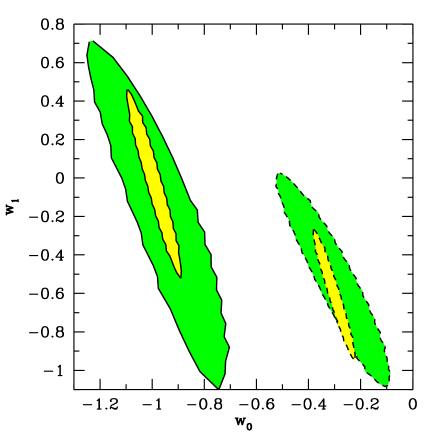
In fig. 20 we show the results of these specifications for the $\Lambda$ model, the periodic potential (dashed line) and the SUGRA inspired model (dotted line). In the left panel we plot the $99\%$ joint probability regions for the linear fit with a fixed prior on $\Omega_{\rm m}$. With NGST specifications we can not establish evolution even for the strongly evolving periodic potential model. If we study the constant fit with no constraints on $\Omega_{\rm m}$ (right panel) we can not improve current bounds on $\Omega_{\rm m}$ as given in [59]. We have not included the systematic error of this measurement in the analysis, which makes the results even more spread out. Altogether it seems clear that a refined low redshift measurement together with the NGST can not provide the same information concerning dark energy models as SNAP, although NGST can complement SNAP in the high redshift region. This leaves the question open if there are surveys which exploit different physics to gain information about the dark energy content of the universe. One possibility are future galaxy cluster surveys [93] either with an Sunyaev Zel’dovich or an X-ray survey. The analysis for these surveys in the context of dark energy has only been performed for constant $w_{\phi}$ models. The $3\sigma$ errors for the joint probabilities in the $\Omega_{\rm m}$-$w_{0}$ plane for a X-ray survey have roughly the same size as for the SNAP specification in fig. 13. It is interesting that these methods seem to be complementary to the SNAP observations in the sense that the error contours are nearly perpendicular to each other [97]. One of the main drawbacks of this method is the unknown evolution of cluster luminosity-temperature relation. How an evolving $w_{\phi}$ could influence the estimation of parameters with galaxy cluster abundance is not clear and should be included in a future analysis. A different method was proposed in [97] which exploits galaxy counts with the planned Deep Extragalactic Evolutionary Probe (DEEP) survey[98]. This survey gives roughly the same error contours as the ones we present in fig. 13. Again the analysis of this survey has not included an evolving $w_{\phi}$ model. Further possibilities to constrain dark energy could be the Alcock-Paczynski test [99, 100], the evolution of density perturbations [44], gravitational waves [101], lensing surveys or observations of the Lyman-$\alpha$ forest [102].

VIII Conclusions

We have investigated the prospects of future supernova experiments to pin down the nature of the dark energy. We have emphasized the importance of choosing a good parameterization scheme for the different dark energy models, concluding that parameterizing the equation of state of the dark energy is the most powerful known method, because the magnitude-redshift functions $m(z)$ which result give the best fits to most of the dark energy models actually proposed. There are two caveats worth noting here. Firstly, there might be an even better parameterization scheme out there that has yet to be discovered (that provides even better fits). Secondly, this scheme is unlikely to provide good fits to all possible models (the periodic model is an example). The ultimate test for a given model is to simply generate $m(z)$ for that model and compare it with the data.

We then use the proposed SNAP satellite as case study for what might be possible with improved datasets. In three recent publications by I. Maor et al. [86], P. Astier [87] and our own [88] the prospect of the SNAP mission have been briefly discussed. Maor et al. [86] argue that SNAP can not distinguish different dark energy models and that it is nearly impossible to reconstruct evolution of the equation of state of the dark energy component. Ours and P. Astier’s [87] results agree with their findings, but as seen in figs. 13 and 19, we show that if we constrain the analysis to a constant $w_{\phi}$ then it is well within the scope of SNAP to distinguish dark energy models, even if we do not impose any priors on $\Omega_{\rm m}$. If it is possible to exploit the full precision of the SNAP instrument ($\sigma_{\rm mag}=0.09\,{\rm mag}$) and to constrain $\Omega_{\rm m}$ to $0.05$, then it is even possible to reconstruct evolution at the $3\sigma$ level as long as the linear evolution today is above the $|w_{1}|>0.6$ threshold. These results are confirmed by [87]. As a conclusion we can say that SNAP certainly has the ability to distinguish dark energy models from a cosmological constant and possible can put some constraints on the evolution of the equation of state of the scalar field component. Whether or not alternative surveys, like a X-ray or SZ survey [93] or the DEEP survey [97] can achieve the same accuracy is currently under investigation.

REFERENCES

- [1] S. Perlmutter et al., Ap. J. 483, 565 (1997).
- [2] A. Riess et al., Astron. J 116, 1009 (1998).
- [3] S. Perlmutter et al., Ap. J. 517, 565 (1999).
- [4] A. Einstein, Sitzungsberichte der Preussischen Akad. d. Wiss. , 142 (1917).
- [5] A. Einstein, Sitzungsberichte der Preussischen Akad. d. Wiss. , 235 (1931).
- [6] G. Gamow, My world line (New York: Viking Press, 1970).
- [7] W. de Sitter, MNRAS 78, 3 (1917).
- [8] Ya. B. Zel’dovich, Sov. Phys. Usp. 11, 381 (1968).
- [9] S. Weinberg, Rev. Mod. Phys. 61, 1 (1989).
- [10] S. M. Carroll, Living Rev. Rel. 4, 1 (2001).
- [11] S. Perlmutter, M. S. Turner and M. White, Phys. Rev. Lett. 83, 670 (1999).
- [12] P. de Bernadis, Nature 404, 955 (2000).
- [13] A. E. Lange et al., Phys. Rev. D63, 042001 (2001).
- [14] C. B. Netterfield et al., astro-ph/0104460.
- [15] P. de Bernadis et al., Ap. J. 564, 559 (2002).
- [16] S. Hanany et al., Ap. J. Lett. 545, 5 (2000).
- [17] A. Balbi et al., Ap. J. Lett. 545, 1 (2000).
- [18] R. Stompor et al., Ap. J. Lett. 561, 7 (2001).
- [19] N. W. Halverson et al., astro-ph/0104489.
- [20] C. Pryke et al., astro-ph/0104490.
- [21] J. J. Mohr, B. Mathiesen and A. E. Evrard, Ap. J. 517, 627 (1999).
- [22] S. Dodelson and L. Knox, Phys. Rev. Lett. 84, 3523 (2000).
- [23] M. Reuter and C. Wetterich, Phys. Lett. B188, 38 (1987).
- [24] R. D. Peccei, J. Sola and C. Wetterich, Phys. Lett. B195, 183 (1987).
- [25] C. Wetterich, Nucl. Phys. B302, 668 (1988).
- [26] P. J. E. Peebles and B. Ratra, Ap. J. 325, L17 (1988).
- [27] B. Ratra and P. J. E. Peebles, Phys. Rev. D37, 3406 (1988).
- [28] C. Wetterich, Astron. Ap. 301, 321 (1995).
- [29] J. Frieman et al., Phys. Rev. Lett. 75, 2077 (1995).
- [30] K. Coble, S. Dodelson and J. A. Frieman, Phys. Rev. D55, 1851 (1997).
- [31] P. G. Ferreira and M. Joyce, Phys. Rev. Lett. 79, 4740 (1997).
- [32] P. G. Ferreira and M. Joyce, Phys. Rev. D58, 023503 (1998).
- [33] E. J. Copeland, A. R. Liddle and D. Wands, Phys. Rev. D57, 4686 (1998).
- [34] R. R. Caldwell, R. Dave and P. J. Steinhardt, Phys. Rev. Lett. 80, 1582 (1998).
- [35] I. Zlatev, L. Wang and P. J. Steinhardt, Phys. Rev. Lett. 82, 896 (1999).
- [36] P. J. Steinhardt, L. Wang and I. Zlatev, Phys. Rev. D 59, 123504 (1999).
- [37] P. Binétruy, Phys. Rev. D60, 063502 (1999).
- [38] Ph. Brax and J. Martin, Phys. Lett. B 468, 40 (1999).
- [39] K. Choi, Phys. Rev. D62, 043509 (2000).
- [40] A. Albrecht and C. Skordis, Phys. Rev. Lett. 84, 2076 (2000).
- [41] See at: http://snap.lbl.gov
- [42] Y. Wang, Ap. J. 531, 676 (2000).
- [43] P. M. Garnavich et al., Ap. J. 509, 74 (1998).
- [44] A. A. Starobinsky, JETP Lett. 68, 721 (1998).
- [45] G. Efstathiou, MNRAS 310, 842 (1999).
- [46] D. Huterer and M. S. Turner, Phys. Rev. D60, 081301 (1999).
- [47] T. D. Saini et al., Phys. Rev. Lett. 85, 1162 (2000).
- [48] T. Nakamura and T. Chiba, Ap. J. 550, 1 (2001).
- [49] Y. Wang, Ap. J. 552, 445 (2001).
- [50] V. Trimble, Rev. Mod. Phys. 54, 1183 (1982).
- [51] V. Trimble, Rev. Mod. Phys. 55, 511 (1983).
- [52] S. E. Woosley and T. A. Weaver, ARA & A 24, 205 (1986).
- [53] R. Barbon, F. Ciatti and L. Rosino, Astron. Ap. 25, 241 (1973).
- [54] Y. P. Pskovskii, Sov. Astron. 21, 675 (1977).
- [55] Y. P. Pskovskii, Sov. Astron. 28, 658 (1984).
- [56] M. M. Phillips, Ap. J. Lett. 413, 105 (1993).
- [57] M. Hamuy, Astron. J 106, 2392 (1993).
- [58] G. Efstathiou et al., astro-ph/0109152.
- [59] N. Bahcall and X. Fan, Ap. J. 504, 1 (1998).
- [60] J. Carlstrom et al., in “Particle Physics and the Universe” (Nobel Symposium 1999), edited by L. Bergstrom, P. Carlson and C. Fransson, (World Scientific 1999).
- [61] G. Efstathiou, J. Bond and S. White, MNRAS 258, 1 (1992).
- [62] See at http://www.sdss.org/sdss.html
- [63] See at http://sirtf.caltech.edu/
- [64] A. Guth, Phys. Rev. D23, 347 (1981).
- [65] A. Albrecht and P. J. Steinhardt, Phys. Rev. Lett. 48, 1220 (1982).
- [66] A. D. Linde, Phys. Lett. 108B, 389 (1982).
- [67] C. Kolda and D. H. Lyth, Phys. Lett. B 458, 197 (1999).
- [68] P. Brax, J. Martin and A. Riazuelo, hep-ph/0104240.
- [69] J. Weller, in “7th International Symposium on Particles, Strings and Cosmology” (2000), edited by K. Cheung, J. F. Gunion and S. Mrenna, (World Scientific 2000).
- [70] J. Barrow, R. Bean and J. Magueijo, MNRAS 316, L41 (2000).
- [71] G. Dvali and S. H. H. Tye, Phys. Lett. 450B, 72 (1999).
- [72] C. Skordis and A. Albrecht, astro-ph/0012195.
- [73] T. Barreiro, E. J. Copeland and N. J. Nunes, Phys. Rev. D61, 127301 (2000).
- [74] S. Dodelson, M. Kaplinghat and E. Stewart, Phys. Rev. Lett. 85, 5276 (2000).
- [75] J. P. Uzan, Phys. Rev. D59, 123510 (1999).
- [76] T. Chiba, Phys. Rev. D60, 083508 (1999).
- [77] R. Bean and J. Magueijo, Phys. Lett. B517, 177 (2001).
- [78] L. Amendola, Phys. Rev. D62, 043511 (2000).
- [79] L. Amendola and D. Tocchini-Valentini, Phys. Rev. D64, 043509 (2001).
- [80] T. Chiba, T. Okabe and M. Yamaguchi, Phys. Rev. D62, 023511 (2000).
- [81] C. Armendariz-Picon, V. Mukhanov and P. J. Steinhardt, Phys. Rev. Lett. 85, 4438 (2000).
- [82] B. Boisseau et al. , Phys. Rev. Lett. 85, 2236 (2000).
- [83] V. Barger and D. Marfatia, Phys. Lett. B498, 67 (2001).
- [84] D. Huterer and M. S. Turner, astro-ph/0006419.
- [85] T. Chiba and T. Nakamura, Phys. Rev. D62, 121301 (2000).
- [86] I. Maor, R. Brustein and P. J. Steinhardt, Phys. Rev. Lett. 86, 6 (2001).
- [87] P. Astier, astro-ph/0008306.
- [88] J. Weller and A. Albrecht, Phys. Rev. Lett. 86, 1939 (2001).
- [89] W. Press et al., Numerical Recipes in FORTRAN: The Art of Scientific Computing (Cambridge University Press, 1986).
- [90] G. Cowan, Statistical Data Analysis (Oxford University Press, 1998).
- [91] D. Huterer and M. S. Turner, Phys. Rev. D64, 123527 (2001).
- [92] G. P. Holder et al., Ap. J. 544, 629 (2000).
- [93] Z. Haiman, J. J. Mohr and G. P. Holder, Ap. J. 553, 545 (2001).
- [94] V. Sahni and A. Starobinsky, Int. J. Mod. Phys. D9, 373 (2000).
- [95] R. Caldwell, astro-ph/9908168.
- [96] J. R. Bond, G. Efstathiou and M. Tegmark, MNRAS 291, L33 (1997).
- [97] J. A. Newman and M. Davis, Ap. J. Lett. 534, 11 (2000).
- [98] See at http://www.ucolick.org/deep/
- [99] C. Alcock and B. Paczynski, Nature 281, 358 (1979).
- [100] N. Dalal et al., Phys. Rev. Lett. 87, 141302 (2001).
- [101] Z. H. Zhu, M. K. Fujimoto abd D. Tatsumi, Astron. Ap. 372, 377 (2001).
- [102] M. Tegmark, astro-ph/0101354.