Analysis of two quintessence models
with SN Ia data

Abstract

The supernovae Ia data are used to analyze two general exact solutions for quintessence models. The best fit values for $\Omega_{m0}$ are smaller than in the $\Lambda$-term model, but still acceptable. With present-day data, it is not possible to discriminate among the various situations.

1 Introduction

Recently, astronomers discovered an accelerated expansion of our Universe. It is well known that all known types of matter generate attraction, which leads to a decelerated expansion of the Universe. That discovery then reveals a new type of matter, which is now called quintessence or, sometimes, dark energy (Ostriker and Steinhardt, 1995; Turner and White, 1997; Chiba et al., 1997; Caldwell et al., 1998; Zlatev et al., 1999; Perlmutter et al., 1999,b).

The discovery of the presence of dark energy became possible when astronomers recognized that SN Ia can be the long expected standard candle for cosmological investigations. Two main features provide the use of SN Ia as a standard candle (Filippenko and Riess, 2000):

i) They are exceedingly luminous, comparable with luminosity of a whole galaxy; they can, thus, be detected and observed with high S/N ratio even at cosmological distances.

ii) “Normal” SNe Ia have small variations among their peak absolute magnitudes (around 0.3).

The accelerated expansion of our Universe was discovered as a result of two projects: the High-z SN Search (Schmidt et al., 1998; Riess et al., 1998) and the Supernova Cosmology Project (Perlmutter et al., 1999,a).

In fact, a new type of matter was predicted many years ago by A. Einstein, who included a $\Lambda$-term into his considerations (Einstein, 1917). At the beginning of the past century, the $\Lambda$-term was just a new fundamental constant, and only much later it was really considered as a formidable challenge by both observational and theoretical cosmologists (Weinberg, 1989; Dolgov et al., 1990; Zel’dovich, 1992; Carroll et al., 1992; Carroll, 2000; Sahni and Starobinsky, 2000; Rubakov, 2000). Moreover, during the last 20 years cosmologists understood that this constant can be replaced with a scalar field, which induces the repulsive gravitational force dynamically. Accordingly, several models were proposed (Ratra and Peebles, 1988; Peebles and Ratra, 1988; Wetterich, 1995, 1998; Copeland et al., 1998; Ferreira and Joyce, 1998; Liddle and Scherrer, 1999; Steinhardt et al., 1999; Brax and Martin, 1999; Sahni and Wang, 2000; Binetruy, 2000; Rubano and Scudellaro, 2001), in order to explain the observed present acceleration of our Universe.

Two of these models continued to be developed after the discovery of acceleration, and were also roughly elaborated and adapted for present-day data (Rubano and Scudellaro, 2001). Here, we again use these models to such an end, but in a much more refined way: the goal is now to fit the observed data of apparent magnitude and redshift of the supernovae Ia, and test the models themselves.

2 Model description

As said above, in this paper we discuss two models for quintessence, both based on a scalar field with a special type of potential. The field is minimally coupled with pressureless matter, and the total density parameter $\Omega$ of the Universe is fixed to be 1. A detailed discussion of the consequences of assuming such models in cosmology is given in (Rubano and Scudellaro, 2001), so that we limit ourselves here only to a short summary of the results we need for our purpose.

The main attractive feature of these models is that they allow a general exact solution of the field equations, obtained through a suitable transformation of variables. Anyway, independently of the fact that this is an exact solution, we also find that this solution reflects many properties of the real Universe correctly.

The first model considers a potential of the form

$$V(\varphi)=B^{2}e^{-\sigma\varphi},$$ (1)

where $B^{2}$ is a generic positive constant and $\sigma^{2}$ is some fixed combination of universal constants

$$\sigma^{2}={\frac{\displaystyle 12\pi G}{\displaystyle c^{2}}}.$$ (2)

Actually, this kind of potential has already been widely discussed in the literature, but without any particular assumption on the value of $\sigma$ (Ratra and Peebles, 1988; Peebles and Ratra, 1988; Wetterich, 1995, 1998; Copeland et al., 1998; Ferreira and Joyce, 1998; Brax and Martin, 1999; Sahni and Wang, 2000; Binetruy, 2000; Fabris et al., 2000). We stress that it is the particular choice of this constant given above that allows the exact integration of the field equations (see also (Barrow, 1987; Burd and Barrow, 1988)).

The general solution of the cosmological equations (both for the metric and the scalar field) has five free parameters (including $B^{2}$) (Rubano and Scudellaro, 2001). We fix two of them and keep three as free. But one of these three parameters just determines the present value of the scale factor of our Universe, which, in a spatially flat geometry, is not observable. It is not included into statistical analysis and does not affect the degrees of freedom of our analysis.

We list below only the three cosmological functions which we need in our analysis (the other ones can be found in (Rubano and Scudellaro, 2001), of course)

$$(1+z)^{3}={\frac{\displaystyle\tau^{2}_{0}(1+\tau^{2}_{0})}{\displaystyle\tau^{2}(1+\tau^{2})}},$$ (3)

$$H={\frac{\displaystyle 2(1+2\tau^{2})}{\displaystyle 3t_{s}\tau(1+\tau^{2})}},$$ (4)

$$\Omega_{m}={\frac{\displaystyle 1+\tau^{2}}{\displaystyle(1+2\tau^{2})^{2}}}.$$ (5)

They are the redshift of the epoch, the Hubble parameter, and the $\Omega_{m}$ parameter of pressureless matter, and are expressed in terms of the dimensionless time $\tau\equiv t/t_{s}$. The free parameters are then the time scale $t_{s}$ and the present value of the dimensionless time $\tau_{0}$. Le us remark that $t_{s}$ is of the same order of magnitude (but not necessary equal to) as the age of the Universe.

As to the second model, it considers a potential of the form

$$V(\varphi)=A^{2}e^{\sigma\varphi}+B^{2}e^{-\sigma\varphi},$$ (6)

with $\sigma^{2}=12G\pi/c^{2}$ as before, and $A^{2}$ and $B^{2}$ free parameters.

We have, now, one additional free parameter; therefore, according to the same considerations as above, we have to deal with three of them.

The equations which describe the Hubble parameter, the redshift, and the density parameter in the second model are

$$(1+z)^{3}={\frac{\displaystyle\lambda^{2}\sinh^{2}\tau_{0}\sin^{2}\tau_{0}}{\displaystyle\lambda^{2}\sinh^{2}\tau-\sin^{2}\tau}},$$ (7)

$$H(\tau)={\frac{\displaystyle\omega(\sin(2\tau)-\lambda^{2}\sinh(2\tau))}{\displaystyle 3(\sin^{2}\tau-\lambda^{2}\sinh^{2}\tau)}},$$ (8)

$$\Omega_{m}(\tau)={\frac{\displaystyle 2(\lambda^{2}-1)(\cos(2\tau)+\lambda^{2}\cosh(2\tau)-1-\lambda^{2})}{\displaystyle(\sin(2\tau)-\lambda^{2}\sinh(2\tau))^{2}}}.$$ (9)

The dimensionless time, in this case, is $\tau=\omega t$. Following Rubano and Scudellaro (2001), we use here $\omega$ instead of $t_{s}$, because of the fact that it is directly connected with the parameters in the potential of the scalar field, and has the meaning of a mass factor in theoretical considerations. So, the free parameters are $\omega$, $\lambda$, and $\tau_{0}$.

In the analysis of the supernovae data, we use the bolometric distance. As explained better below, it can be expressed in terms of the “Hubble free” luminosity distance and of a parameter $m_{0}$, connected with the absolute magnitude and the Hubble parameter. The parameters of the first model ($\tau_{0}$ and $t_{s}$) can be recasted into $\tau_{0}$ and $m_{0}$. The parameters of the second model ($\lambda$, $\tau_{0}$, and $\omega$) can be recasted into $\lambda$, $\tau_{0}$, and $m_{0}$. Once the best fit is made, it is easy to compute the relevant physical quantities $H_{0}$ and $\Omega_{m0}$. In all the considerations below, $H_{0}$ turns out to have the same value as in (Perlmutter et al., 1999,a). So, we concentrate on $\Omega_{m0}$.

3 SNe Ia Data

The published data of the supernovae consist of 60 SNe Ia (Perlmutter et al., 1999,a). The data analysis and the determination of cosmological parameters can be considered in two steps. The first one is the measurement of the Hubble parameter for close supernovae (Calan - Tololo survey) (Hamuy et al., 1996), to be compared with the absolute magnitude $M$ of a supernova SN Ia. The second step is the comparison of the high redshift supernovae with the theoretical prediction of bolometric distance:

$$m=5\log(D_{b})+m_{0};$$ (10)

here, $D_{b}$ is the ”Hubble free” bolometric distance

$$D_{b}=H_{0}(1+z)\int^{z}_{0}\frac{dz^{\prime}}{H(z^{\prime})},$$ (11)

and $m_{0}$ is a parameter connected to the absolute magnitude and the Hubble parameter.

In data presented in (Perlmutter et al., 1999,a) there are several values for corrected apparent magnitude. Authors consider $m^{peak}_{B}$ and stretch luminosity corrected effective $B$-band magnitude $m^{eff}_{B}$. For the analysis of cosmological parameters only $m^{eff}_{B}$ is used, together with its errors $\sigma_{m_{B}^{eff}}$.

There are several methods for SN Ia data analysis. Two of them are used in (Riess et al., 1998). The first one is the Multicolor Light Curve Shape (MLCS) method and the second one is a template fitting method. In (Perlmutter et al., 1999,a) another method is used.

The data of both groups have the statistical errors approximately as $\sigma_{m}\sim 0.25$.

We follow the authors of paper (Perlmutter et al., 1999,a) to analyze the models described in (Rubano and Scudellaro, 2001). First of all, as a check of the procedure, we apply the flat cosmological model with a $\Lambda$-term to fit the data. The standard $chi^{2}$ algorithm of data analysis reveals a good agreement of our analysis with published statistical values (Perlmutter et al., 1999,a). We use the complete set of data of 60 SNe Ia. It results $\chi^{2}=1.75$ per degree of freedom, not significantly different from $\chi^{2}=1.76$ found in (Perlmutter et al., 1999,a). The same is for the $\Omega_{\Lambda}$ parameter. Since 4 points in the data are outliers, we can proceed with analysis and exclude these data from our considerations. The total number of SN Ia data then drops to 56. The $\chi^{2}$ per degree of freedom in this case becomes 1.16, which is in good agreement with previously published results (Perlmutter et al., 1999,a) and is within $1\sigma$ level.

4 Data analysis and fitting

In our analysis we use the standard $\chi^{2}$ method. The analysis is done minimizing the value of weitghed $\chi^{2}$:

$$\chi^{2}=\sum w_{i}(m_{i}-m^{model}_{i})^{2},$$ (12)

where $w_{i}$ is the weight of the $i$-th SN Ia, $m_{i}$ is its $B$-band effective apparent magnitude, and $m^{model}_{i}$ is its magnitude as predicted with the models introduced before and thoroughly discussed in (Rubano and Scudellaro, 2001).

4.1 The first model

In the first model, it is possible to eliminate $\tau$ from Eqs. (3) and (4), and to obtain an analytical expression for $H(z)$. Thus, it is possible to compute $m$ from Eqs. (10) and (11), and $\chi^{2}$ as a function of $\tau$ and $m_{0}$.

Firstly, we use 60 SN Ia data and get the $\chi^{2}$ minimum at $m_{0}=24.01$, $\tau_{0}=1.04$, with $\chi^{2}=1.77$ per degree of freedom. As it is unsatisfactory, we reject data which are out of the 3$\sigma$ level, as done in (Perlmutter et al., 1999,a).

After data rejection, the $\chi^{2}$ minimum drops down to $\chi^{2}=1.195$ per degree of freedom. It is definitely within one sigma level of the expected value of $\chi^{2}$. The minimum now has other values than $m_{0}=23.985$ and $\tau_{0}=1.268$.

If we accept the value of this minimum, we obtain, from Eqs. (4) and (5), $H_{0}=70kms^{-1}Mpc^{-1}$, $\Omega_{m0}=0.15$.

The situation is illustrated in Figs. 1 – 3.

4.2 The second model

The second model has only been tested and fitted with 56 data of SNe Ia. The number of parameters in this case is equal to three. The true minimum of the $\chi^{2}$ is at $m_{0}=23.98$, $\tau_{0}=0.8$, and $\lambda=1.182$. We find a value of $\chi^{2}=1.1906$, which is definitely within one sigma level of expected value. After such value we obtain from Eqs. (8) and (9) that $\Omega_{m0}=0.17$.

The $\chi^{2}$ value is a function of three arbitrary values: $m_{0}$, $\tau_{0}$, and $\lambda$. Therefore, the $\chi^{2}$ as a function of all parameters is impossible to plot, but we can nonetheless plot several slits.

The situation is illustrated in Figs. 4 – 8.

5 Conclusions

In a quintessential universe we have analyzed the same data as in (Perlmutter et al., 1999,a), where it is present only a cosmological constant, and found good values for $\chi^{2}$ in both cases. The values of $\Omega_{m0}$ found are rather different from the one found in (Perlmutter et al., 1999,a), but it is impossible to say if this is due to differences in the models or to influence of the measurement errors on the final values.

In fact, in both models we have degeneracy in the parameters, particularly large in $\lambda$ (II model). This makes impossible to give significant confidence limits for the values of $\Omega_{m0}$, which we found. Only very rough estimates can be given. Our main results are summarized in the following tables.

Model I

$\chi^{2}$	$m_{0}$	$\tau_{0}$	$\Omega_{m0}$	$\tau_{0}$ range	$\Omega_{m0}$ range
1.195	23.985	1.268	0.15	0.82 $\div$ 1.40	0.12 $\div$ 0.30

Model II

$\chi^{2}$	$m_{0}$	$\tau_{0}$	$\lambda$	$\Omega_{m0}$	$\Omega_{m0}$ range
1.19	23.98	0.8	1.182	0.17	0.14 $\div$ 0.22

As final remarks, we want to observe that our results are in a very good agreement with the one found in (Bahcall et al., 2000) in a completely independent way, and that the high degeneracy we get for the model parameters seems to support the opinion of those who claim that it is very difficult to discriminate among theories on the basis of observational data only (Maor et al., 2000; Barger and Marfatia, 2000).

Figure 1: The surface of $\chi^{2}$ as a function of two variables, the $\tau_{0}$ parameter and $m_{0}$ parameter. This function has a very definite and sharp minimum.

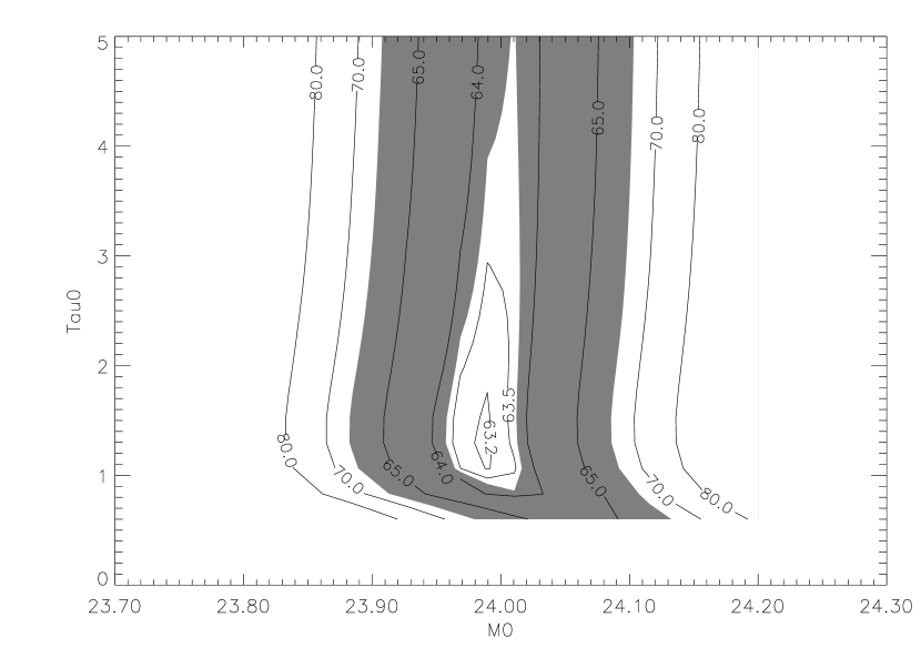
Figure 2: Countour plot of the levels of $\chi^{2}$ is shown. The one sigma level is the small white region on the graph. The two sigma level is the shadowed region. It reveals a large degeneracy of the $\chi^{2}$ function with respect to the parameter $\tau_{0}$.

Figure 3: The solid line corresponds to the slit of 2D $\chi^{2}$ taken at the point of true minimum $m_{0}=23.985$. The dot-and-dashes curves corresponds to the slit taken at $m_{0}=24.035$, and the dashes curve to the slit taken at $m_{0}=23.935$. It results that the minimum in $\tau_{0}$ is strongly dependent on the $m_{0}$ minimum.

Figure 4: The surface of $\chi^{2}$ as a function of two parameters: $m_{0}$ and $\lambda$; here, we fix $\tau_{0}=0.8$. One can see the profile of this surface and minimum.

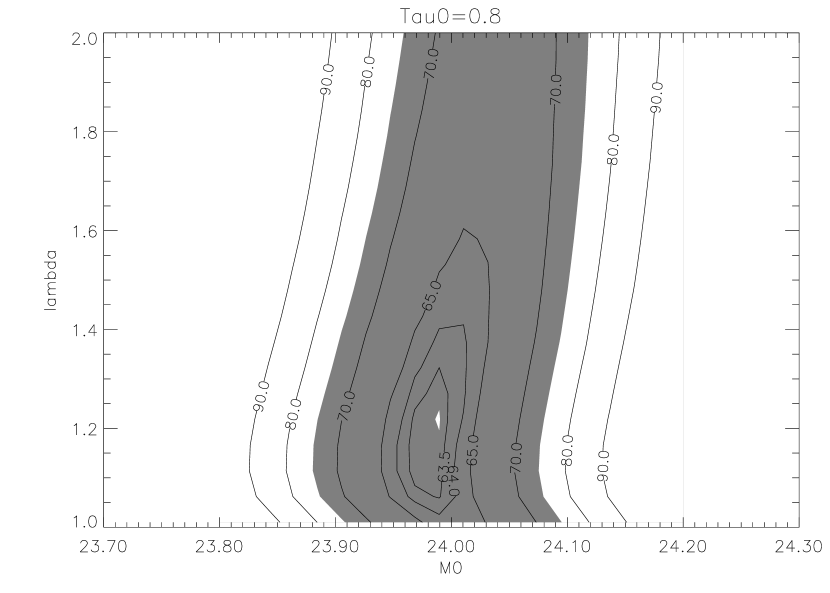
Figure 5: Contour plot of the Fig. 4 surface. The 1$\sigma$ area is the small white region at $m_{0}=23.985$ and at $\tau_{0}=1.268$. The shadowed region is the $2\sigma$ area, revealing that there is parameter degeneracy.

Figure 6: We plot $\chi^{2}$ as a function of other two parameters, $\tau_{0}$ and $\lambda$, fixing $m_{0}=23.985$.

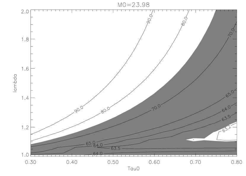
Figure 7: Countour plot of Fig. 6 surface. The white region in the right corner below is the $1\sigma$ level of parameters $\tau_{0}$ and $\lambda$. The shadowed region is the $2\sigma$ level of these parameters. One can see again a large degeneration for them.

Figure 8: Three different slits at fixed $m_{0}=23.985$ and $\tau_{0}=0.8$, showing degeneracy in $\lambda$.

References

- Bahcall et al. (2000) Bahcall, N. et al., ApJ, 541, 1
- Barger and Marfatia (2000) Barger, V. and Marfatia, D. 2000, astro-ph/0009256
- Barrow (1987) Barrow, J. D. 1987, Phys. Lett. B, 187, 12
- Binetruy (2000) Binetruy, P. 2000, hep-th/0005037
- Brax and Martin (1999) Brax, Ph. and Martin, J. 1999, Phys. Lett. B, 468, 40
- Burd and Barrow (1988) Burd, A. B. and Barrow, J. D. 1988, Nucl. Phys. B, 308, 929
- Caldwell et al. (1998) Caldwell, R. R., Dave, R., and Steinhardt, P. J. 1998, Phys. Rev. Lett., 80, 1582
- Carroll (2000) Carroll, S. M. 2000, astro-ph/0004075.
- Carroll et al. (1992) Carroll, S. M., Press, W. H., and Turner, E. L. 1992, Ann. Rev. Astron. Astrophys., 30, 499
- Chiba et al. (1997) Chiba, T., Sugiyama, N., and Nakamura, T. 1997, MNRAS, 289, L5
- Copeland et al. (1998) Copeland, E. J., Liddle, A. R., and Wands, D. 1998, Phys. Rev. D, 57, 4686
- Dolgov et al. (1990) Dolgov, A. D., Sazhin, M. V., and Zel’dovich, Ya. B. 1990, Basics of modern cosmology, Gif-sur-Yvette: Editions Frontieres, 1990
- Einstein (1917) Einstein, A. 1917, Sitzungber. Preuss. Akad. Wiss. Phys.-Math. Kl., 142
- Fabris et al. (2000) Fabris, K. C., Goncalves, S. V. B., and Tomimura, N. A. 2000, Class. Quantum Grav., 17, 2983
- Ferreira and Joyce (1998) Ferreira, P. G. and Joyce, M. 1998, Phys. Rev. D, 58, 023503
- Filippenko and Riess (2000) Filippenko, A. V. and Riess, A. G. 2000, “Type Ia Supernovae and Their Cosmological Implications”, in: Type Ia Supernovae: Theory and Cosmology, J.C. Niemeyer, J.W. Truran (eds.), Cambridge: Cambridge Univ. Press, 2000, 1
- Hamuy et al. (1996) Hamuy, M. et al., Astron. J., 112, 2391
- Liddle and Scherrer (1999) Liddle, A. R. and Scherrer, R. J. 1999, Phys. Rev. D, 59, 023509
- Maor et al. (2000) Maor, I., Brunstein, R., and Steinhardt, P. J. 2000, astro-ph/0007297
- Ostriker and Steinhardt (1995) Ostriker, J. P. and Steinhardt, P. J. 1995, Nature, 377, 600
- Peebles and Ratra (1988) Peebles, P. J. E. and Ratra, B. 1988, ApJ, 325, L17
- Perlmutter et al. (1999,a) Perlmutter, S., Aldering, G., Goldhaber, G. et al. 1999, ApJ, 517, 565
- Perlmutter et al. (1999,b) Perlmutter, S., Turner, M. S., and White, M. 1999, Phys. Rev. Lett., 83, 670
- Ratra and Peebles (1988) Ratra, B. and Peebles, P. J. E. 1988, Phys. Rev. D, 37, 3406
- Riess et al. (1998) Riess, A. G., Filippenko, A. V., Challis, P. et al. 1998, Astron. J., 116, 1009
- Rubakov (2000) Rubakov, V. A. 2000, Phys. Rev. D, 61, 061501
- Rubano and Scudellaro (2001) Rubano, C. and Scudellaro, P. 2001, astro-ph/0103335, to appear in General Relativity and Gravitation
- Sahni and Starobinsky (2000) Sahni, V. and Starobinsky, A. 2000, Int. J. Mod. Phys. D, 9, 373
- Sahni and Wang (2000) Sahni, V. and Wang, L. 2000, Phys. Rev. D, 62, 103517
- Schmidt et al. (1998) Schmidt, B. P., Suntzeff, N. B., Phillips, M. M. et al. 1998, ApJ, 507, 46
- Steinhardt et al. (1999) Steinhardt, P. J., Wang, L., and Zlatev, I. 1999, Phys. Rev. D, 59, 123504
- Turner and White (1997) Turner, M. S. and White, M. 1997, Phys. Rev. D, 56, 4439
- Weinberg (1989) Weinberg, S. 1989, Rev. Mod. Phys., 61, 1
- Wetterich (1995) Wetterich, C. 1995, Astron. Astrophys., 301, 321
- Wetterich (1998) Wetterich, C. 1998, Nucl. Phys. B, 302, 668
- Zel’dovich (1992) Zel’dovich, Ya. B. 1992, My Universe: selected reviews, Zel’dovich, Ya. B. and Sazhin, M. V. (eds.), Gordon and Breach, 1992
- Zlatev et al. (1999) Zlatev, I., Wang, L., and Steinhardt, P. J. 1999, Phys. Rev. Lett., 82, 896