L-dwarf variability: Magnetic star spots or non-uniform clouds?
Abstract
The recent discovery of photometric variations in L dwarfs has opened a discussion on the cause of the variations. We argue against the existence of magnetic spots in these atmospheres and favor the idea that non-uniform condensate coverage (i.e. clouds) is responsible for the variations. The magnetic Reynolds number () in the atmosphere of L dwarfs, which describes how well the gas couples with the magnetic field, is too small (1) to support the formation of magnetic spots. In constrast silicate and iron clouds form in the photospheres of L dwarfs. Inhomogeneities in such cloud decks can plausibly produce the observed photometric variations. Further evidence in support of clouds is the tendency for variable L dwarfs to be bluer in than the average L dwarf of a given spectral type. This color effect is expected if clear holes appear in an otherwise uniform cloud layer.
1 Introduction
Like stars of earlier spectral types, some L dwarfs (the spectral type cooler than M; Kirkpatrick et al., 1999; Martín et al., 1999; Basri et al., 2000; Kirkpatrick et al., 2000) are variable (Tinney & Tolley, 1999; Bailer-Jones & Mundt, 1999, 2001). In this Letter we examine whether magnetic ‘star’ spots or clouds are more likely to be responsible for the observed variability. We conclude that patchy clouds are the most plausible mechanism for the observed variability and discuss how they can produce the three types of variations seen: 1) periodic, 2) periodic but periods change on long time scales (months), and 3) non-periodic.
Tinney & Tolley (1999) presented the first attempt to detect clouds in brown dwarf atmospheres. They observed the M9 brown dwarf LP944-20 and the L5 brown dwarf DENIS 1228-15 through two narrow-band filters designed to detect changes in TiO absorption. The changes in the TiO band strength were presumed to indicate changes in the opacity, which occurs when TiO is depleted through condensation. They found that LP944-20 was variable, but DENIS 1228-15 was not. The authors speculated that the passage of clouds over the disk of LP944-20 produced small changes in the effective temperature that caused the small variations (0.04 magnitude) in their narrow-band filters. These results do not exclude the possibility of clouds in their L dwarf, however, since variations of this amplitude would have been difficult to detect given that the errors for that object were larger than 0.04 magnitude.
Bailer-Jones & Mundt (1999) conducted a variability search in the broad-band filter and found evidence of variability in the L1.5 dwarf 2MASS 1145+23. The object displayed 0.04 magnitude variations that repeated with a period of 7.1 hours. In an expanded study of 21 L and M dwarfs Bailer-Jones & Mundt (2001) found that over half of their sample exhibited statistically significant variations with amplitudes 0.01 to 0.055 magnitude and time scales of 0.4 to 100 hours. They were unable to find periodic light curves for many of the variables. 2MASS 1145+23, however, now exhibited variability with a period of 11.2 hrs. A similar varying period has also been observed in an M9.5 dwarf star by Martín, Zapatero Osorio, & Lehto (2001), who suggested that evolving surface features, possibly dust clouds or magnetic spots, were responsible for the change.
At first glance, either magnetic spots or clouds could plausibly be associated with the observed variability. Magnetic fields have been measured for several M dwarfs and estimates of their strength are a few kG (Saar, 1994; Johns-Krull & Valenti, 1996). The surface filling factors are generally . Unfortunately, periodic photometric variations have been observed in only a few M dwarfs, suggesting that either the surfaces of these objects are completely covered with spots or that the spots are few in number and uniformly distributed (Hawley, Reid, & Gizis, 2000). In addition, Bondar (1995) reports that no good data exist to support the scenario of cyclic, organized spots in objects cooler than M0.
For the L dwarfs, clouds are also a reasonable potential source of variability. Iron, enstatite, and forsterite are the most abundant species expected to condense at the atmospheric temperatures and pressures characteristic of the L dwarfs (Lodders, 1999; Burrows & Sharp, 1999). Once condensed, the species likely settle into discrete, optically thick, cloud decks, with optically thicker clouds arising in progressively later L dwarfs (Marley, 2000; Ackerman & Marley, 2001). Since the atmospheric circulation pattern of most L dwarfs is likely similar to that of Jupiter (Schubert & Zhang, 2000) it is not unreasonable to expect that many L dwarfs also have a banded appearance. Any large inhomogeneities (thicker clouds or holes in the cloud deck) could then produce a photometric signal. Gelino & Marley (2000) have shown that if Jupiter was an unresolved point source, the Great Red Spot would provide a photometrically detectable signal. If L dwarfs have similar cloud features to Jupiter, then it is plausible that they may also exhibit photometric variations. The observation that more of the later L dwarfs are variable than the earlier type (Bailer-Jones & Mundt, 2001) supports the scenario of cloud-caused variations.
In addition to the photometric variability, some L dwarfs exhibit H emission (Kirkpatrick et al., 1999, 2000), which is known to be an indicator of high chromospheric temperatures and magnetic activity in earlier type stars (Hawley et al., 2000). If the variability in L dwarfs is caused by magnetic spots, then it is plausible to expect a correlation between H emission and the variable objects. Gelino et al. (in preparation) have combined their L-dwarf photometric variability results with those of Bailer-Jones & Mundt (2001) and find no correlation between H emission (i.e. magnetic activity) and variability, supporting the conclusions of Bailer-Jones & Mundt (2001) and Martín et al. (2001).
As with earlier-type stars, wave heating has been suggested as the mechanism responsible for producing hot brown dwarf upper atmospheres (Yelle, 2000). Convection-caused waves propagate and grow as they rise through the upper atmosphere, eventually releasing their energy and heating the gas as they dissipate. These high temperatures combined with magnetic field effects are likely responsible for the H emission. L dwarfs with weak magnetic fields should exhibit little or no H emission. In light of this it is quite notable that the fraction of objects with H emission peaks at spectral type M7 and decreases at earlier and later spectral types (Gizis et al., 2000). No L dwarfs later than L5 show H in emission (Kirkpatrick et al., 2001), although one T dwarf does (Burgasser et al., 2000). Since the early L population consists of both young brown dwarfs and old stars, this trend could indicate an inability of either substellar objects or cool stars to produce magnetic fields appropriate to maintain the H emission (Gizis et al., 2000).
Using kinematics as a probe for age, Gizis et al. (2000) have argued that the old stellar L-dwarf population is more likely to show H emission than the younger, lower mass population. This might imply that the process by which H emission is produced is driven by the mass of the object and not the effective temperature. Indeed, the dissipation of acoustic waves in the upper atmosphere could be responsible for the heating of the chromosphere. Unfortunately, this process is poorly characterized at the masses and effective temperatures of interest here.
In addition to H emission, radio emission can also be a signature of a magnetic field. Berger et al. (2001) recently reported the detection of a radio flare as well as quiescent emission from the M-dwarf LP944-20. They infer that the radio emission is caused by synchrotron emission and estimate a field strength of 5 G, much less than the field strengths of active M dwarfs (Haisch, Strong, & Rodono, 1991). In addition the substellar nature, old age (Tinney, 1998), and rapid rotation (Tinney & Reid, 1998) all support the weak field strength; many L dwarfs with spectroscopically determined rotation velocities are rotating quite rapidly and lack significant H emission (Hawley et al., 2000), suggesting that the magnetic fields of these presumably old objects are too weak to slow down the rotation.
The existence of a magnetic field in LP944-20 is also supported by the observation of an X-ray flare (Rutledge et al., 2000). An X-ray flare in an old, non-accreting object such as this can only be caused by magnetic activity. However, the lack of quiescent X-ray emission suggests that the magnetic field is quite weak. Rutledge et al. postulate that because of the rapid rotation in this object, either the turbulent dynamo is being suppressed or the magnetic field is being configured into a more organized form. They also suggest that the lack of ionization in the cool photosphere prevents the magnetic field from coupling with the gas in the atmosphere, causing the field to dissipate.
Fleming, Giampapa, & Schmitt (2000) arrive at the same conclusion with their study of the X-ray flare of the M8 dwarf VB 10. They go so far as to estimate the ionization fraction in its atmosphere, by extrapolating the ionization fractions in the atmospheres of early dwarfs down to the effective temperature of VB 10. They estimate that the ionization fraction in late M dwarfs is 2 orders of magnitude lower than in early M dwarfs and 3 orders of magnitude smaller than in the sun, and conclude that that magnetic footprints (i.e. spots) are unlikely to exist in the photosphere. By way of comparison, the cooler M9 dwarf LP944-20 is even less likely to have magnetic spots than VB 10, supporting the conclusion by Tinney & Tolley (1999) that they were detecting the signature of clouds. This, in turn, implies that magnetically produced spots are unlikely to be formed in L dwarfs and the variations seen by Bailer-Jones & Mundt (2001) and Gelino et al. (in preparation) are caused by clouds.
In this Letter we further explore the possibility that the magnetic field and atmospheric gas in L dwarfs are not coupled. We improve on the estimations of Fleming et al. (2000) by utilizing models of the abundances of ions and neutrals appropriate for L-dwarf atmospheres.
2 Magnetic Spots
Magnetic spots in the sun (i.e. sunspots) are thought to form as magnetic flux tubes rise to the photosphere (Parker, 1955). For magnetic buoyancy to be important, the plasma must be a sufficiently good conductor. This criterion is most likely not satisfied in cool L-dwarf atmospheres, especially in the low pressure regions where the temperatures are also low. In these regions the free electron abundance is extremely small ( cm-3 above 1 bar for a 2000 K model), therefore, the regions do not make good conductors. Consequently, it would seem that this condition alone prevents the formation of any magnetic spots.
To estimate the strength of coupling between the gas and the magnetic field we compute the magnetic Reynolds number for L-dwarf atmospheres. is a dimensionless parameter describing how efficiently a gas interacts with a magnetic field; (Priest, 1982), where is a length scale, is a velocity scale, and is the magnetic diffusivity of the gas. When 1, the magnetic field slips through the gas with no interaction; for 1, the magnetic field is frozen in the gas.
To compute we rely on atmosphere models computed by Marley et al. (2001) for cloudy L dwarfs. The models employ the cloud model of Ackerman & Marley (2001) with the cloud parameter . The L-dwarf range is still uncertain, but likely lies between about 2200 and 1300 K. We consider models with of 2000 to 1200 K and surface gravity of cm s-2, appropriate for a Jupiter mass brown dwarf.
The appropriate length scale to use in the calculation of is not obvious. In the area around sunspots, is usually taken as the size of the sunspot, a small fraction of the solar radius. We choose to set , the pressure scale height. Typical values of are around 106 cm at the 1 bar level. For the velocity scale we use the convective velocity of the atmosphere, , as computed in Ackerman & Marley (2001) and references therein. Ackerman & Marley limit the size of above the radiative-convective boundary. To compute an upper limit to we compute assuming that the entire thermal flux of the brown dwarf is carried by convection throughout the atmosphere. Typical convective velocities are computed to be 103-104 cm s-1.
The value for is computed from Priest (1982); , where is a factor to account for the partial ionization of the plasma, is temperature, is the number density of neutral atoms and molecules, is the number density of electrons, and is the Coulomb logarithm. We use the abundance tables of Lodders (1999) to calculate and . The appropriate value of the Coulomb logarithm, however, is not known for an L-dwarf atmosphere. Table 2.1 from Priest (1982) gives the value of for temperatures and densities relevant for the sun. Unfortunately, this table provides no entries at the densities and temperatures needed for the extrapolation to the parameters of an L-dwarf atmosphere since becomes small (). However, Chen (1974) comments that it is sufficient to use =10 regardless of the specific plasma parameters. This is well supported from the data in the table in Priest since only varies from over 15 orders of magnitude in density and 3 orders of magnitude in temperature. We use a value of 5 for our calculations, but test the sensitivity of on our somewhat arbitrarily chosen value by computing with at the unrealistic values of 1 and 100. We find that computed at these limits differs by for our coolest model and for our warmest model and stress that for the region of parameter space covered by our calculation the precise value of is essentially irrelevant.
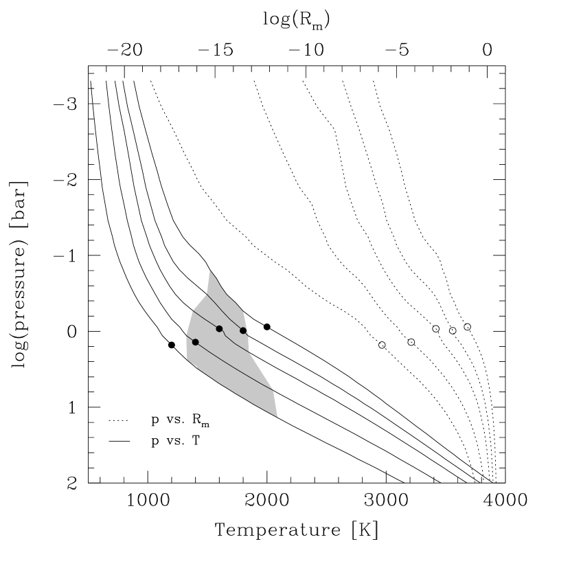
The value of as a function of pressure in the model atmospheres is shown in Figure 1. is very small throughout the entire upper atmosphere; only at pressures of and higher does start to approach 1. By comparison, near sunspots is estimated to be 104-106 (Priest, 1982). Open circles denote the approximate base of the photosphere (where ) for the models shown. Note that in contrast to the sun, only approaches unity well below the photosphere. At =1, the plasma and the magnetic field will interact with each other only to a small degree. Any weak magnetic disturbances deep in these atmosphere are unlikely to affect the surface thermal flux since the winds and weather patterns alluded to earlier will redistribute the upwelling thermal flux before it is radiated. Thus, throughout the atmospheres of L dwarfs, spanning the range from roughly L2 to L8 (Kirkpatrick et al., 1999, 2000) we expect little or no interaction between the atmosphere and the magnetic field.
3 Clouds
The thermal fluxes emerging from L-dwarf atmospheres are affected by clouds. Early L dwarfs have relatively thin clouds high in the atmosphere (Ackerman & Marley, 2001). Figure 1 illustrates the trend for the clouds to form progressively deeper in the atmosphere at later spectral types. Again the base of the photosphere is marked for the models shown. Unlike the case for , the clouds form in the immediate vicinity of the photosphere and thus are well placed to affect the emitted thermal flux. For objects with (approximately L2 and cooler; Stephens et al., 2001) clouds play an important role in the emitted flux since the condensate opacity is significant.
For an arbitrary L dwarf the emitted flux in some spectral regions will be limited by the cloud deck, while in others gaseous opacity reaches optical depth unity above the cloud. Marley et al. (2001) illustrate the effects of gaseous and condensate opacity for a variety of L dwarfs. If there is a transitory clearing in the cloud deck additional flux will emerge from those spectral regions in which the cloud opacity is otherwise dominant. Examples are the peaks of flux emerging from the water band windows in z, J, H, and bands and the optical flux in band. The resulting bright spots on the objects will be similar to the ‘5-m hot spots’ of Jupiter (Westphal, Matthews, & Terrile, 1974) where flux emerges from holes in the ammonia cloud. An atmosphere with such non-uniformly distributed high contrast regions is quite capable of producing photometric variations.
As cloud optical thickness increases with later spectral type, L-dwarf color becomes redder, eventually saturating around 2 (Marley, 2000; Allard et al., 2001; Ackerman & Marley, 2001; Marley et al., 2001; Tsuji, 2001). Clouds in cooler objects lie well below the photosphere, and leave the radiating region in the atmosphere relatively clear. The clear atmosphere partially manifests itself in the blue seen in the T dwarfs (Allard et al., 1996; Marley et al., 1996; Tsuji et al., 1996).
These trends suggest that infrared colors of variable objects may support the cloud model for variability. The color of those objects which have been surveyed for variability is shown in Figure 2. Although subject to small number statistics, suspected variables with spectral types later than L2 tend to be bluer than the average L dwarf (Kirkpatrick et al., 2000) at the same spectral type. Models predict (Marley, 2000; Marley et al., 2001) that a hypothetical L dwarf with no clouds will be substantially bluer ( mag; Marley & Ackerman, 2001) at than a more realistic object with the same effective temperature and a cloudy atmosphere. Thus, if the average L dwarf at a given spectral type is entirely covered with clouds, it would not likely be seen as a variable and it would have more typical color. In order for photometric variations to arise by the cloud mechanism there must be non-uniformity in the cloud coverage, such as clearings in the clouds. So, not only would clear sections of the atmosphere (holes) provide a source for brightness variations, flux emerging through the hypothetical holes would cause the color to be somewhat bluer than the average object. The lack of a similar trend for the early L and late M dwarfs might indicate a different mechanism is at work in those atmospheres. Clearly more data, including time resolved multi-color photometry, are required to determine if variability is indeed connected to color.
Schubert & Zhang (2000) show that the atmosphere of L dwarfs can exist in one of two states, chaotic or banded. Since clouds respond to atmospheric motions, they would presumably reflect one of these two morphologies. In general, higher mass objects will have more chaotic and three-dimensional internal dynamics than lower mass objects, meaning that the higher mass objects are less likely to have banded cloud features. It is not obvious which cloud morphology would better produce photometric variations. For example, objects with more chaotic atmospheres might be more likely to have uniformly distributed clouds. When rotating such objects might show little photometric variation. If the chaotic atmospheres result in fairly complete cloud coverage, then we might expect that more massive L dwarfs would be redder in and tend not to be variable. Conversely, if chaotic atmospheres more often produce large holes in the clouds they may more easily produce photometric signatures than banded atmospheres. In this scenario, the more massive L dwarfs would be bluer in and tend to be variable. Furthermore, rapidly evolving, chaotic atmospheres may be responsible for the changes in photometric period observed for some objects. It is easy to imagine similar scenarios for banded clouds.
The presence of clouds can also explain the different types of variability seen in L dwarfs. For example, periodic variations over time scales of days can be explained by a long-lived clearing or thickening in the clouds. Rotation modulation of the photometric signal will then produce a periodic signal. The inhomogeneities could migrate latitudinally or dissipate and reform at a different latitude as does the Great Dark Spot in the atmosphere of Neptune (Hammel & Lockwood, 1997). If wind speed is a function of latitude as on all the giant planets of our solar system, then spots at different latitudes will circle the object with different periods. Observations taken several months apart will show periodic variations with different periods as is reported for the L-dwarf 2MASS 1145+23. Finally, L dwarfs whose clouds change on time scales of a few days or less or whose cloudy spots are distributed at several latitudes with different wind speeds could still produce a photometric signal, but the signal might not be periodic. Clearly, more observations and modeling are required to better characterize atmospheric circulation and weather in L-dwarf atmospheres.
4 Conclusions
There is little doubt that some L dwarfs are photometrically variable. Although most authors suggest that the variations are caused by clouds, the possibility of magnetic spots is often mentioned (e.g. Bailer-Jones & Mundt, 1999, 2001; Martín et al., 2001). We have shown that the low ionization fraction predicted by L-dwarf models and the accompanyingly low magnetic Reynolds numbers strongly argue against spots as a possible cause for the photometric variations. On the other hand silicate and iron grains condense in L-dwarf atmospheres within the photosphere. These clouds are likely responsible for the photometric variations discovered in the various studies, particularly for the later L dwarfs (about L2 and later). Since the thermal emission of T dwarfs is also influenced by clouds (Marley et al. 2001) we predict that variability will also be found in the opacity window regions of these objects. Further work with models and more observations are clearly needed to better understand cloud composition and dynamics.
References
- Ackerman & Marley (2001) Ackerman, A. S., & Marley, M. S. 2001, ApJ in press (astro-ph/0103423)
- Allard et al. (1996) Allard, F., Hauschildt, P. H., Baraffe, I., & Chabrier, G. 1996, ApJ, 465, L123
- Allard et al. (2001) Allard, F., Hauschildt, P. H., Alexander, D. R., Tamanai, A., & Schweitzer, A. 2001, ApJ in press (astro-ph/0104256)
- Bailer-Jones & Mundt (1999) Bailer-Jones, C. A. L. & Mundt, R. 1999, A&A, 348, 800
- Bailer-Jones & Mundt (2001) Bailer-Jones, C. A. L. & Mundt, R. 2001, A&A, 367, 218
- Basri et al. (2000) Basri, G., et al. 2000, ApJ, 538, 363
- Berger et al. (2001) Berger, E., et al. 2001, Nature, 410, 338
- Bondar (1995) Bondar, N. I. 1995, A&AS, 111, 259
- Burgasser et al. (2000) Burgasser, A. J., Kirkpatrick, J. D., Reid, I. N., Liebert, J., Gizis, J. E., & Brown, M. E. 2000, AJ, 120, 1100
- Burrows & Sharp (1999) Burrows, A., & Sharp, C. M. 1999, ApJ, 512, 843
- Chen (1974) Chen, F. F. 1974, Introduction to Plasma Physics (New York: Plenum Press)
- Fleming et al. (2000) Fleming, T. A., Giampapa, M. S., & Schmitt, J. H. M. M. 2000, ApJ, 533, 372
- Gelino & Marley (2000) Gelino, C. R., & Marley, M. S. 2000, in ASP Conf. Ser. 212, From Giant Planet to Cool Stars, ed. C. A. Griffith & M. S. Marley (San Francisco: ASP), 322
- Gizis et al. (2000) Gizis, J. E., Monet, D. G., Reid, I. N., Kirkpatrick, J. D., Liebert, J., & Williams, R. J. 2000, AJ, 120, 1085
- Haisch, Strong, & Rodono (1991) Haisch, B., Strong, K. T., & Rodono, M. 1991, ARA&A, 29, 275
- Hammel & Lockwood (1997) Hammel, H. B., & Lockwood, G. W. 1997, Icarus, 129, 466
- Hawley et al. (2000) Hawley, S. L., Reid, I. N., & Gizis, J. E. 2000, in ASP Conf. Ser. 212, From Giant Planets to Cool Stars, ed. C. A. Griffith & M. S. Marley (San Francisco: ASP), 252
- Johns-Krull & Valenti (1996) Johns-Krull, C. M., & Valenti, J. A. 1996, ApJ, 459, L95
- Kirkpatrick et al. (1999) Kirkpatrick, J. D., et al. 1999, ApJ, 519, 802
- Kirkpatrick et al. (2000) Kirkpatrick, J. D., et al. 2000, AJ, 120, 447
- Kirkpatrick et al. (2001) Kirkpatrick, J. D., Dahn, C. C., Monet, D. G., Reid, I. N., Gizis, J. E., Liebert, J., & Burgasser, A. J. 2001, AJ in press (astro-ph/0103218)
- Lodders (1999) Lodders, K. 1999, ApJ, 519, 793
- Marley (2000) Marley, M. S. 2000, in ASP Conf. Ser. 212, From Giant Planets to Cool Stars, ed. C. A. Griffith & M. S. Marley (San Francisco: ASP), 152
- Marley & Ackerman (2001) Marley, M. S., & Ackerman, A. S. 2001, proceedings of IAU Symposium 202, “Planetary Systems in the Universe: Observation, Formation and Evolution” in press (astro-ph/0103269)
- Marley et al. (1996) Marley, M. S., Saumon, D., Guillot, T., Freedman, R. S., Hubbard, W. B., Burrows, A., & Lunine, J. I. 1996, Science, 272, 1919
- Marley et al. (2001) Marley, M. S., Seager, S., Saumon, D., Lodders, K., Ackerman, A. S., & Freedman, R. 2001, ApJ submitted (astro-ph/0105438)
- Martín et al. (1999) Martín, E. L., Delfosse, X., Basri, G., Goldman, B., Forveille, T., & Zapatero Osorio, M. R. 1999, AJ, 118, 2466
- Martín et al. (2001) Martín, E. L., Zapatero Osorio, M. R., & Lehto, H. J. 2001, ApJ in press (astro-ph/0104377)
- Parker (1955) Parker, E. N. 1955, ApJ, 121, 491
- Priest (1982) Priest, E. R. 1982, Solar Magnetohydrodynamics (Dordrecht, Holland: D. Reidel Publishing)
- Rutledge et al. (2000) Rutledge, R. E., Basri, G., Martín, E. L., & Bildsten, L. 2000, ApJ, 538, L141
- Saar (1994) Saar, S. H. 1994, in IAU Symp. 154, Infrared Solar Physics, ed. D. M. Rabin et al. (Dordrecht: Kluwer), 493
- Schubert & Zhang (2000) Schubert, G., & Zhang, K. 2000, in ASP Conf. Ser. 212, From Giant Planets to Cool Stars, ed. C. A. Griffith & M. S. Marley (San Francisco: ASP), 210
- Stephens et al. (2001) Stephens, D., Marley, M., Noll, K., & Chanover, N. 2001, ApJ, in press
- Tinney (1998) Tinney, C. G. 1998, MNRAS, 296, L42
- Tinney & Reid (1998) Tinney, C. G., & Reid, I. N. 1998, MNRAS, 301, 1031
- Tinney & Tolley (1999) Tinney, C. G., & Tolley, A. J. 1999, MNRAS, 304, 119
- Tsuji (2001) Tsuji, T. 2001, Proceedings of the IAU Workshop on “Ultracool Dwarfs: Surveys, Properties and Spectral Classification” ed. H. R. A. Jones & I. Steele, in press
- Tsuji et al. (1996) Tsuji, T., Ohnaka, K., Aoki, W., & Nakajima, T. 1996, A&A, 308, L29
- Westphal, Matthews, & Terrile (1974) Westphal, J. A., Matthews, K., & Terrile, R. J. 1974, ApJ, 188, L111
- Yelle (2000) Yelle, R. V. 2000, in ASP Conf. Ser. 212, ¿From Giant Planets to Cool Stars, ed. C. A. Griffith & M. S. Marley (San Francisco: ASP), 267